Gravitationalconstants IU2

IU2

Modul Universal constants

Gravitational constants

In addition to his formulation of the law of motion I

N

’

,

perhaps his greatest contribution to physics was the discovery of the gen-

eral common law of gravitation. It describes the interaction between be-

tween two bodies, planets, or even smaller particles that causes a move-

ment that can be described by the K

’

Laws. The law was formu-

lated in 1666 by N

and 1687 was published as a chapter of his

monumental work Philosophiae Naturalis Principia Mathematica.

In addition to his formulation of the law of motion ISSACNEWTON’S, perhaps his greatest con- tribution to physics was the discovery of the general common law of gravitation. It describes the interaction between between two bodies, planets, or even smaller particles that causes a move- ment that can be described by the KEPLER’SLaws. The law was formulated in 1666 by NEWTON

and 1687 was published as a chapter of his monumental workPhilosophiae Naturalis Principia Mathematica.

c

AP, Departement Physik, Universität Basel, July 2020

1.1 Preliminary Questions

• How is inertia defined?

• What is torsion?

• What is torque?

• What is the unit of the gravitational constant?

• How does the experiment of Cavendish function?

• What is harmonic motion?

• What is the corresponding equation of motion?

• What happens when a shaft is drilled through the center of the earth and a ball is tossed in?

1.2 Theory

1.2.1 Newton’s law of gravity

K

’

second law states that the force with which the gravitational interaction is associ- ated with is a central force. This means that the force acts along a connection line between the centers of two interacting bodies. If we assume that the gravitational interaction is a general property, we must on the other hand consider the force F, which is associated with the inter- action and is proportional to the "amount" of matter in any body, and the proportion of the corresponding masses m

and m

. We can therefore write:

F = m

· m

· f ( r ) (1.1)

It is difficult to determine the dependence of the force F on the distance r. Basically, the de- pendence is determined experimentally by the force between the masses m

and m

and is measured at different distances, whereby the relationship between F and r can finally be de- rived. Such experimental determination is indeed possible. However, it requires sensitive measuring equipment and relatively large patience. However, N

had no such exper- imental possibilities. He recognized, motivated by K

laws as the law of gravity had to be designed to:

The gravitational interaction between two bodies, by a central attraction, is ex- pressed that the masses of the bodies are directly proportional and the square of the distance between them is inversely proportional.

Or something more modern terms:

F = γ · ^m

· m

r

(1.2)

wherein γ is the proportionality or gravitational constant. However, with Eq. 1.2, the two

interacting bodies are to be understood as point masses. For the description of planetary

orbits, while the expansion of the planet is neglected, since these are small compared to the

radii of the planetary orbits.

1.2.2 The Experiment of Cavendish

The core piece of the gravitational balance from Cavendish is on a thin torsion hairline cross- bar suspended horizontally and at each end at a distance d, a suspension point carries a small lead ball of mass m

. These balls are big two lead balls tightened of mass m

according to Eq.

(1.2). Although this force is less than 10

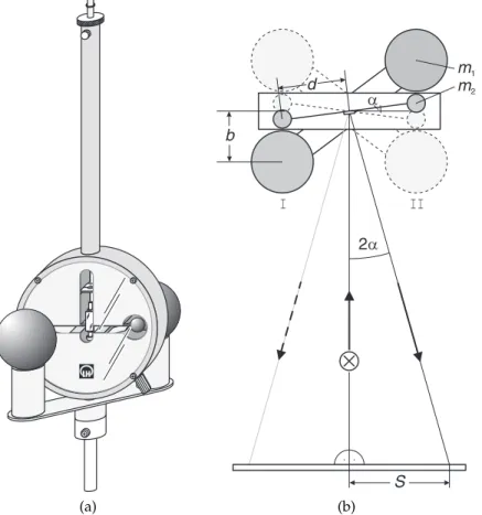
N, it can be detected with an extremely sensitive torsional balance. Motion observed the movement of the small lead balls and is measured via a laser pointer (see Fig. 1.1)

(a) (b)

Figure 1.1: gravitation torsional balance from Cavendish (left) and schematic illustration of the laser pointer (right).

This is made by means of an illuminated concave mirror and is fixed rigidly to the crossbar of the torsional pendulum. From the chronological course of the movement, the mass m

and the geometry of the arrangement is determined on the basis of the gravitational constant from the following considerations in the next section.

1.2.3 Determination of the gravitational constant

The gravitational force between two lead balls of mass m

and m

at a distance b according to Eq. (1.2) is:

F

= γ m

m

b

, (1.3)

when the large lead balls are in position I (see Fig. 1.1), thus acting on the torsion pendulum

4

of the torque:

M

= 2Fd = 2γ m

m

b

d (1.4)

This will be compensated by the restoring moment of the torsion wire, so that the pendulum assumes an equilibrium α

. This means that the torque M

can also be written as

M

= − Dα

(1.5)

with D being the torsion coefficient of the suspending wire. By swirling the big balls in posi- tion I I, it can now force about the symmetrical, so that a torque M

= − M

is now effective and the damped oscillations of the pendulum can perform about the new equilibrium position α

. The difference between the two torques is given by:

M

− M

= M

− (− M

) = 2M

= 4γ m

m

b

d

= − Dα

− (− Dα

) = D ( α

− α

)

(1.6) It immediately follows

4γ m

m

b

d = D ( α

− α

) (1.7)

The torsion coefficient D can be derived with the solution to the equation of motion for a damped torsion pendulum (see Appendix). One gets

D = 4π

T

+ δ

J = ( 4π

+ T

δ

) J

T

(1.8)

with T being the oscillation period, δ being the decay constant of the damped oscillation and J being the moment of inertia of the torsion pendulum. The latter can be approximated by taking both small lead balls as point masses and neglecting the masses of all other parts of the torsion pendulum (crossbar, mirror, suspending torsion wire). This leads to

J = 2m

d

(1.9)

It follows for Eq. (1.8):

D = ² ( 4π

+ T

δ

) m

d

T

(1.10)

Plugging this into Eq. (1.7) and solving for the gravitational constant yields γ = ( 4π

+ T

δ

) b

d

2m

T

( α

− α

) (1.11)

1.2.4 Measurement of the rotation angle α

In Fig. 1.1, the measurement of the rotation angle α is described with the help of the laser pointer. The illumination beam of the laser pointer is perpendicular here to the zero position of the torsional pendulum (the rest position without large lead balls). The laser pointer position for the zero is in line with the zero scale agreement. Between the rotation angle α, the laser pointer position S, and the distance L

between the scale and torsion, the connection is:

tan ( 2α ) = ^S

L

(1.12)

Figure 1.2: Scheme for determining the deflection of the laser pointer.

for small angles α, respectively:

α = ^S

2L

(1.13)

In Fig. 1.2, the concave mirror is illuminated below the horizontal angle β.

The laser pointer position O for the zero point of the torsional pendulum has the distance L

to the receiving point N of the normal and the distance to the concave mirror:

L = q

L

+ L

. (1.14)

For rotation of the torsion pendulum at the angle α from the zero position, the relationship is found as:

S

= L tan ( 2α ) (1.15)

and

S

S = ^sin ( 90

− β − 2α )

sin ( 90

+ 2α ) = cos ( β ) − tan ( 2α ) sin ( β ) (1.16) The angle α is in any case very small (it is at most 1.5

), the dimensions of the gravitational torsion balance can not be illumination at the angle β above 30

. Therefore, the approximation:

S

S = cos ( β ) = ^L

L (1.17)

is allowed. With the additional approximation tan ( 2α ) ≈ 2α, thus follows the total : α = ^S

2 L

L

+ L

(1.18)

6

This equation (1.18) is subjected to a systematic error 1 − 2%, by the calculation of the differ- ence between the two positions of equilibrium α

− α

and this systematic error will all but almost be completely compensated.

For the special case of illumination with β at small angles and L

≫ L

, one obtains from Eq.

(1.18) the already derived equation (1.13).

Eq. (1.18) is also valid when the illumination beam is tilted up or down. It depends also in this case, on the horizontal reading scale and can be disregarded from the laser pointer.

The zero position of the torsion pendulum, the point O in Fig. 1.2, is usually unknown in front of the enforcement. To determine L

, one measures, in good approximation, the distance between the normal point N and the laser pointer position for the equilibrium position I . This approximation is permitted because of | α | ≪ 1. When oblique illumination is not in the direc- tion of the concave mirror, i.e. for β ≪ 1, L

= 0 can be accepted.

With these thoughts to the rotation angle α, for the experimental setup in Fig. 1.1, Eq. (1.13) can be put into Eq. (1.11). This yields

γ = ( 4π

+ T

δ

) b

d 4m

T

L

( S

− S

) (1.19)

Analogus for the experimental setup in Fig. 1.2, Eq. (1.18) can be plugged into Eg.(1.11) to yield

γ = ( 4π

+ T

δ

) b

dL

4m

T

( L

+ L

) ( S

− S

) (1.20) 1.2.5 Counter torque of the second lead ball

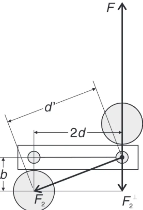
In addition to the torque by the attractive force F of the opposing large lead ball (distance b) is a counter torque through the attraction force F

of the respective distant ball (distance d

) is generated (see Fig. 1.3).

Figure 1.3: Scheme for calculating the counter torque by the "second" lead ball.

Hence, the torque M

, is more exactly than given in Eq. (1.4):

M

= 2 ( F − F

) d (1.21)

From the geometry of the setup in Fig. 1.3 follows F

= F

b

d

(1.22)

The force F

can be found by expressing both, F and F

with Newton’s law of gravity, solving both for the gravitational constant and then setting them equal:

F = γ m

m

b

⇔ γ = ^Fb

2

m

m

F

= γ m

m

d

⇔ γ = ^F

^d

′2

m

m

⇒ F

= F b

d

(1.23)

Putting Eq. (1.23) in Eq. (1.22), and then the resulting equation into Eq. (1.21), one finds for M

:

M

= 2F ( 1 − ^b

3

d

) d (1.24)

The parameter d

can be retrieved immediately from the geometry of Fig. 1.3:

d

= q

( 2d )

+ b

(1.25)

By comparing Eq. (1.24) with Eq. (1.4), it is clear that both equations are identical except of the bracket term. This means that analogous to before the same derivation for the gravitational constant can be made, such that Eq. (1.19) and Eq. (1.20) need to be only multiplied by some correction factor K. This leads to following equation for the gravitational constant for the experimental setup in Fig. 1.1:

γ = ( 4π

+ T

δ

) b

d 4m

T

L

( S

− S

) K (1.26)

and to

γ = ( 4π

+ T

δ

) b

dL

4m

T

( L

+ L

) ( S

− S

) K (1.27) for the experimental setup in Fig. 1.2, whereas

K = ¹ 1 −

and d

= q

( 2d )

+ b

(1.28)

1.3 Experiment

1.3.1 Experimental Data

Parameter Value

Mass of the large ball 1500 g ± 10 g

Distance of the small balls from the point of suspension 4.94 cm ± 0.01 cm Distance of the small balls from the large ball 4.85 cm ± 0.01 cm Distance of the suspension point of the wire to the scale 277 cm ± 0.5 cm

8

1.3.2 Experimental Setup and Adjustment

• For at least two hours ensure there is no vibration before making the arrangement blank so that the pendulum may swing into the equilibrium position.

• Control the stability of the zero point.

• Observe zero fluctuations for at least 10 min.

1.3.3 Measurements

Important: While switching the ball carrier, absolutely avoid shocks of the housing, e.g.

by moving the lead balls into the stop.

• Switch on the laser and record the start position of the laser pointer.

• Put the lead balls carefully rotated from position I to position I I and start the stop watch.

• Read the position of the laser pointer on the scale for 30 min at least every 30 seconds, until the oscillation has subsided.

• Wait about 60-90 minutes until the system is in the equilibrium state again.

• Write down again the starting position of the laser pointer.

• Swing the lead ball from position I I back into position I and repeat the measurement.

• Turn off the laser.

1.3.4 Tasks for Evaluation

• Determine the period, the decay constant, and the equilibrium position of the two series of measurements by performing a fit of a corresponding function on the data.

• Determine the gravitational constant, the correction factor, and the corrected gravita- tional constant.

• Make a complete error calculation.

• Compare the literature value to your result.

Hereinafter the expression for the torsion coefficient D, as it appears in Eq. (1.8) will be de- rived.

In a torsion pendulum the torsion is caused by a torque. The pendulum reacts with a restoring moment that counters the torsion. This can be expressed with

M = − D ϕ ( t ) (A.1)

with D being the torsion coefficient and ϕ ( t ) being the rotating angle, dependent on time. But torque is also nothing else than the derivative of angular momentum with respect to time, i.e.

M = ^d

dt L ( t ) = ^d

dt J ω ( t ) = J d

dt ω ( t ) = J d

dt

ϕ ( t ) (A.2)

Because both equations are equal to a torque M, it is allowed to set them equal to receive the equation of motion for a harmonic torsion pendulum:

J d

dt

ϕ ( t ) = − Dϕ ( t ) (A.3)

Introducing friction analogously to a simple gravity pendulum or a spring pendulum, the fric- tion is proportional to the time derivative of ϕ ( t ) . This term supports the restoring moment, such that the equation of motion can be written as:

J d

dt

ϕ ( t ) = −( Dϕ ( t ) + D ^˜ d

dt ϕ ( t )) (A.4)

whereas ˜ D is the damping constant. Rearranging the equation and defining ω

: = D/J, one gets

d

dt

ϕ ( t ) + ^{D ˜} J

d

dt ϕ ( t ) + ω

ϕ ( t ) = 0 (A.5) To solve this differential equation, one can make the ansatz ϕ ( t ) = e

. Plugging it in and rearranging a little leads to

λ

+ ^{D ˜}

J λ + ω

e

= 0 (A.6)

10

This equation is zero if and only if the bracket vanishes. This means that this is a quadratic equation for λ, whose solutions are:

λ

=

−

± r

D J

− 4ω

2 = − ^{D ˜}

2J ± s

D ˜ 2J

− ω

(A.7)

As it is clearly visible, it is reasonable to define a new constant, which will later in the solution to the equation of motion turn out to be the decay constant. Defining:

δ : = ^{D ˜}

2J (A.8)

With this Eq. (A.7) becomes

λ

= − δ ± ^q δ

− ω

(A.9)

Putting Eq. (A.8) back into Eq. (A.5) leads to the well known equation of motion for a damped oscillation:

d

dt

ϕ ( t ) + 2δ d

dt ϕ ( t ) + ω

ϕ ( t ) = 0 (A.10) Looking at Eq. (A.9), there are three possible cases to consider. If δ > _ω

then there is overdamping, if δ = ω

then there is critical damping and if δ < _ω

then there is under- damping. All three cases yield different solutions to the equation of motion Eq. (A.10). But in this experiment there is only the underdamped case observable and thus only this case is of interest here. In this case, the square root becomes complex and one writes at first λ

= − δ − ^q −( ω

− δ

) = − δ − i

q

ω

− δ

to make sure that the radicand is real. Then a solution to the equation of motion can be constructed with the corresponding λ

and the ansatz made for ϕ ( t ) . This way one gets to the following solution for Eq.(A.10):

ϕ ( t ) = Ae

sin ( ωt + φ ) (A.11) where

ω = ^q ω

− δ

= ^2π

T und ω

= s

D

J (A.12)

Rearranging Eq.(A.12) a little leads to the desired expression for the torsion coefficient:

D = 4π

T

+ δ

J (A.13)