Tangent-point self-avoidance energies for curves
Paweł Strzelecki∗, Heiko von der Mosel∗∗
July 1, 2011
Abstract
We study a two-point self-avoidance energyEqwhich is defined for all rectifiable curves in Rnas the double integral along the curve of 1/rq. Hererstands for the radius of the (smallest) circle that is tangent to the curve at one point and passes through another point on the curve, with obvious natural modifications of this definition in the exceptional, non-generic cases. It turns out that finiteness ofEq(γ)for q≥2 guarantees that γ has no self-intersections or triple junctions and therefore must be homeomorphic to the unit circle S1 or to a closed intervalI. Forq>2 the energyEqevaluated on curves inR3turns out to be a knot energy separating different knot types by infinite energy barriers and bounding the number of knot types below a given energy value. We also establish an explicit upper bound on the Hausdorff-distance of two curves inR3 with finiteEq-energy that guarantees that these curves are ambient isotopic. This bound depends only onqand the energy values of the curves. Moreover, for allqthat are larger than the critical exponentqcrit=2, the arclength parametrization ofγ is of classC1,1−2/q, with H¨older norm of the unit tangent depending only onq, the length ofγ, and the local energy. The exponent 1−2/q is optimal.
Mathematics Subject Classification (2000): 28A75, 49Q10, 53A04, 57M25
1 Introduction
Imagine an unknown and possibly quite irregular closed pathΓforming a loop of finite lengthL>0.
Suppose that the only data you can access are the ratios of the squared distance ofΓ(t)from any other positionΓ(s), to the distance of the current (affine) tangent line`(t)from that previous positionΓ(s), i.e., the quotients
2r(Γ(t),Γ(s)):= |Γ(t)−Γ(s)|2
dist(`(t),Γ(s))∈[0,∞] for s<t. (1.1) What can you say aboutΓ? Could it have self-intersections? How regular must it be? In other words, how much information about a closed curve of finite length in Euclidean space is encoded in the relative tangent-point data (1.1)? The answer is: if you can compute an integral mean of some inverse power of all these data and check that it is finite then you can extract essential topological information as well as explicit smoothness properties of the curve!
∗PS and his research is partially supported by the Polish Ministry of Science and Higher Education grant no. N N201 397737 (years 2009-2012).
∗∗HvdM is partially supported by the DFG grant Mo966/4-1.
To make this precise we assume from now on that the pathΓ⊂Rnis a rectifiable curve of finite length, parametrized by arclength on the circleSL∼=R/(LZ)of perimeterL. Hence,Γis a (not nec- essarily injective) Lipschitz continuous mapping with|Γ0|=1 a.e. onSL. Geometrically, the tangent- point function
r(Γ(t),Γ(s)) = |Γ(t)−Γ(s)|2
2 dist(`(t),Γ(s))= |Γ(t)−Γ(s)|
2 sin<)(Γ0(t),Γ(s)−Γ(t)),
involving the tangent line `(t):={Γ(t) +µΓ0(t):µ ∈R} and defined for alls∈SL and almost all t∈SL, determines the radius of the unique circle that is tangent toΓat the positionΓ(t)and passes throughΓ(s). (This radius is set to be zero ifΓ(t) =Γ(s), and is infinite if the vectorΓ(s)−Γ(t)6=0 is parallel to the tangentΓ0(t)).
The only assumption in the result indicated above is finiteness of thetangent-point potential Eq(Γ):=
Z L
0
Z L
0
dsdt
rq(Γ(t),Γ(s)) for someq≥2. (1.2) Theorem 1.1(Finite energy path is a manifold). IfEq(Γ)<∞for some q≥2then the imageΓ(SL)is a one-dimensional topological manifold (possibly with boundary), embedded inRn.
In particular, the image curve has no self-intersections, although there is no chance to deduce injectivity of the arclength parametrizationΓ itself, since the integrand depends only on the image Γ(SL).Take, for example, ak-times covered circle of lengthL/k, for which the integrand is constant, r(Γ(t),Γ(s))≡r0for alls,t∈SL, so that the energy amounts to
Eq(k-times covered circle) =L2 rq0 =k2
Z L/k
0
Z L/k
0
dsdt
rq0 =k2Eq(once-covered circle)<∞.
So the curve cannot be too wild, since it traces a one-dimensional manifold without any non-tangential self-crossings. But without further input it is impossible to guess how many times the image curve has been covered by the parametrization. Moreover,Γ(SL)could form a manifold with boundary, say, a circular arc, withΓ0making an abrupt half-turn at the endpoints of that arc. Mathematically, one can easily reparametrize the manifold to obtain a new injective arclength parametrization withΓ(t)6=Γ(s) for allt6=s,which we will assume from now on.
In light of Theorem1.1the tangent-point potentialEqevaluated on closed curves inR3may serve as a validknot energyas suggested by Gonzalez and Maddocks in [14, Section 6], that is, as a func- tional separating different knot types by infinite energy barriers. It was shown by Sullivan [29, Prop.
2.2] that forq>2 the energyEqblows up on a sequence of smooth knots converging smoothly to a smooth curve with self-crossings. (His proof uses the Taylor formula up to order two for the converg- ing curves, and a uniform bound for the remainders.) As a consequence of our analysis we generalize this result to continuous curves replacing smooth convergence by uniform convergence (see Proposi- tion5.1). ThusEqforq>2 is indeedself-repulsiveorcharge, and hence a knot energy according to the definition given by O’Hara [18, Def. 1.1] (see also Diao, Ernst, and Janse van Rensburg [11] for a grading of energy functionals used in geometrical knot theory). This provides an affirmative answer to an open question posed in [18, Problem 8.1, p. 127]. It also turns out thatEqisstrongforq>2: among all continuous closed curvesγof fixed lengthLandEq(γ)<Ethere are only finitely many knot types, see Proposition5.2. This gives a partial answer to a conjecture expressed by Sullivan in [29, p. 184]
(leaving open the caseq=2, and we do not consider links with more than one component). Both these knot-theoretic results are based on a prioriC1,α-estimates for curves of finiteEq-energy, discussed in more detail later on.
We will show in addition that two curves, whose Hausdorff-distance is bounded above by an explicit small constant depending only on the energy values, are in fact in the same knot class. A qual- itative version of such an isotopy result is well-known in the smooth category; see e.g. [16, Chapter 8], or [2]. Here, however, we have explicit quantitative bounds. Notice also that Hausdorff-distance alone, no matter how small, does not suffice to separate knot classes;1 boundedEq-energy is crucial here.
Theorem 1.2(Isotopy). For any q>2 there is an explicit constant δ(q)>0 depending only on q such that any two closed rectifiable curves with injective arclength parametrizationsΓ1, Γ2, with finiteEq-energy, are ambient isotopic if their Hausdorff-distance is less than
δ(q)max{Eq(Γ1),Eq(Γ2)}−q−21 .
Our proof of Theorem1.2follows closely the arguments of Marta Szuma´nska who proved in her Ph.D. thesis a similar result [30, Chapter 5] for a related three-point potential, theintegral Menger curvature
Mp(Γ):=
Z L 0
Z L 0
Z L 0
dsdtdσ
Rp(Γ(s),Γ(t),Γ(σ)), p>3, (1.3) whereR(x,y,z)denotes the circumcircle radius of three pointsx,y,z in Euclidean space. Essentially one reduces the isotopy question to that between polygons inscribed inΓ1andΓ2, whose edge lengths are solely controlled in terms of the energy. For polygonal knots a similar result is contained in the work of Millet, Piatek, and Rawdon [17, Theorem 4.2], where instead of (1.3), the polygonal thickness of the polygons together with their edge length determines the smallness condition on the Hausdorff distance that guarantees isotopy of two polygonal knots. For general curves, thickness was defined by Gonzalez and Maddocks in [14] as the smallest possible circumcircle radiusR(·,·,·)when evaluated on all triples of distinct curve points. This concept of thickness was used as a tool in variational applications involving curves and elastic rods subject to various topological constraints; see e.g. [15], [7], [21]–[23], [12], [13], and has been studied numerically; see e.g. [19], [8], [9], [1].
The inverse of thickness of a curveΓcan be obtained as limitsMp1/p(Γ)for p→∞, or Eq1/q(Γ) forq→∞.In our papers [26,24,25] we have studied regularizing, self-avoidance and compactness effects of several integral energies, includingMp, which involve, vaguely speaking, various bounds for 1/Runderstood as a function of three variables, including bounds inLp, inLp(X1,L∞(X2))where X1=SLandX2=SL×SL(or vice versa), and in spaces that resemble the classic Morrey spacesLp,λ. In each case we were able to detect similar phenomena: there is a certain limiting exponent for which an appropriate functional is scale invariant, and above this exponent three sorts of effects take place.
First, curves with finite energy have no self-intersections. Second, these energies serve well as knot energies allowing for valuable compactness results for equibounded families of loops in fixed isotopy classes, which is due to the third, the regularizing effect: Curves with finite energy are more regular than initially assumed.
For the present tangent-point potentialEqwe obtain the following regularity theorem, which shows in particular thatΓ0must exist everywhere and be a continuous function with oscillations controlled by the local energy.
Theorem 1.3(Regularity). If q>2and the arclength parametrizationΓ:SL→Rn is chosen to be injective, then Γ is continuously differentiable with a H¨older continuous tangent, i.e., Γis of class
1Consider for example two different torus knots on the surface of a very thin rotational torus; for the classification of torus knots see e.g. Burde and Zieschang [6, Chapter 3.E].
C1,1−(2/q).More precisely, for each q>2there exist two constantsδ(q)>0and c(q)<∞depending only on q such that each injective arclength parametrizationΓwithEq(Γ)<∞satisfies
|Γ0(u)−Γ0(v)| ≤c(q) Z v
u
Z v
u
ds dt r(Γ(s),Γ(t))q
1/q
|u−v|1−2/q (1.4)
for all u,v∈SLwith|u−v| ≤min δ(q)Eq(Γ)−1/(q−2),12diamγ .
The exponent q=2 is a limiting one here. It is relatively easy to use scaling arguments and check that Eq(Γ) =∞for each q≥2 whenΓparametrizes a closed polygonal curve, but polygons have finite energy for all q<2. The resulting H¨older exponent 1−2/qis reminiscent of the classic Sobolev imbedding theorem in the supercritical case: the domain of integration is two-dimensional, and the integrand is related to curvature. ForC2-curves the behaviour of 1/r close to the diagonal of SL×SL (where 1/r might blow up for curves with low regularity) encodes some information about curvature, i.e. about second derivatives of the arclength parametrizationΓ. The point is that we need no information about the existence ofΓ00in order to prove Theorem1.3. A priori, we deal with curves that are rectifiable only, and even the existence ofΓ0 at all parameters cannot be taken for granted.
Note that inequality (1.4) is qualitatively optimal: for curves of classC1,1 the integrand 1/r is bounded, and (1.4) yields then|Γ0(u)−Γ0(v)|.|u−v|sup(1/r)for u,vsufficiently close; nothing stronger can be expected as the familiar example of a stadium curve shows. We discuss other examples briefly at the end of Section6.
Before describing the main ideas of the proof and the structure of the paper we would like to mention that while working on generalizations of self-avoidance energies to surfaces inR3, see [27], which involved a search for suitable integrands, we have realized thatEqis a model energy that might be the easiest one to extend to the fully general case, i.e. to submanifolds of arbitrary dimension and co-dimension [28]. This was one of the motivations to write the present note: to lay out in a simple, relatively easily tractable case all the arguments that should be applicable in much greater generality.
Theorem1.1is obtained as a corollary of a slightly more general result, see Theorem1.4below.
We first prove a technical lemma (see Section 2) which shows how Eq can be used to control the behaviour of the so-called P. Jones’β-numbers,
βγ(x,d):=inf
sup
y∈γ∩B(x,d)
dist(y,G)
d : G is a straight line throughx
, (1.5)
for smalld>0 and closed ballsB(x,d)of radiusdwith centerx. It turns out that ifE2(Γ)<∞then βγ(x,d)→0 as d→0 uniformly with respect to x, see Lemma 2.3 and the remark at the end of Section2. And this is the key point to prove thatγ=Γ(SL)is a topological manifold, as we have the following.
Theorem 1.4. If Γ:SL→Rnis an arclength parametrization, and the imageγ=Γ(SL)satisfies sup
x∈γβγ(x,d)≤ω(d) (1.6)
whereω:[0,L]→Ris a continuous nondecreasing function withω(0) =0, thenγis a one-dimensio- nal submanifold ofRn(possibly with boundary).
The main idea behind the proof of Theorem1.4is simple: if the result were false, then we could find a pointxinγ where a triple junctionoccurs; in a small ballBcentered atxwe would have (at
least) three disjoint arcs ofγin a long narrow tube. Two of them would then be very close (i.e., would leaveBcrossing∂Bin the same spherical cap at one end of the tube). Observing points of those two arcs, and using (1.6) on smaller and smaller scales, we are able to obtain a contradiction and eventually show that there could be no triple junction atx. For details, see Section3.
By the preliminary results of Section2, ifEq(Γ)<∞for someq>2, then the control ofβ numbers is much better than just (1.6). Namely,
sup
x∈γβγ(x,r).rκ (1.7)
forκ= (q−2)/(q+4)<λ =1−2/q; the constant in (1.7) depends onEq(Γ). Applying (1.7) itera- tively, we find in Section4suitably defined cones that contain short arcs ofγ and obtain an estimate for their opening angles, proving thatΓ0exists everywhere and is of class2Cκ.
Section5contains the proof of the isotopy result, Theorem1.2. In the last section we show how to bootstrap the initial gain ofC1,κ-regularity obtained in Section4, to the optimal regularity Γ∈ C1,1−(2/q), and we will establish (1.4). We stress the fact that Inequality (1.4) in Theorem1.3provides a uniform a priori estimate. This can be used in variational applications and to ensure compactness for infinite families of curves with uniformly bounded energy. Some results of that type have been stated in [24,25]; we do not follow that thread here.
Finally, let us say that, at the moment, we do not know howΓ0behaves in the limiting caseq=2 (we do not even know if it is defined everywhere for curves with finiteE2-energy) but we are tempted to think thatΓ0 has vanishing mean oscillation forq=2 and that local oscillations of the tangent can be controlled by the local energy of the curve.
Notation
We writeG(x,y) to denote the straight line through two distinct points x,y∈Rn. If x=Γ(s),y= Γ(t)∈γ :=Γ SL
⊂Rn, then, abusing the notation slightly, we write sometimesG(s,t)instead of G(Γ(s),Γ(t)).
For a closed setFinRnwe set
Uδ(F):={x∈Rn: dist(x,F)<δ}, δ>0.
In some places, it will be more convenient to work directly with the slabsUδ around appropriately selected lines than to deal with the information expressed only in the language ofβ-numbers. Finally, in Section4we work with cones. Forx6=y∈Rnandε∈(0,π2)we denote by
Cε(x;y) :={z∈Rn:∃t6=0 such that <)(t(z−x),y−x)<ε
2} (1.8)
the double cone whose vertex is at the pointx, with cone axis passing through y, and with opening angleε. All ballsB(x,r)with radiusr>0 and centerx∈Rnare closed balls throughout the paper.
2In some cases, uniform estimates ofβ-numbers on a set imply that this set is aC1,κ-manifold; see David, Kenig and Toro [10] and Preiss, Tolsa and Toro [20]. Their results apply to anym-dimensional set inRnthat isReifenberg flat with vanishing constant. But here we have no Reifenberg flatness a priori, as in general rectifiable curves do not have to be Reifenberg flat. In fact, we prove flatness by hand, using energy bounds leading to (1.7).
2 Decay of beta numbers
Lemma 2.1. LetEq(Γ) be finite. There exists a constant c0=c0(q)>0such that ifε <1/200and d<diamγsatisfy
ε4+qd2−q≥c0(q)Eq(Γ), (2.9)
then for every two points of the curve such that|Γ(s)−Γ(t)|=d we have γ∩B2d Γ(s)
⊂ U20εd G(s,t) . In particular,
βγ(Γ(s),2d)≤10ε. Forq>2 we setκ= (q−2)/(q+4).
Corollary 2.2. There exists aδ1=δ1(q)>0such that ifEq(Γ)1/(q+4)dκ<δ1, then βγ(Γ(s),2d)≤c1(q)Eq(Γ)1/(q+4)dκ.
Proof of Lemma2.1.Fors,t∈SL,d=|Γ(s)−Γ(t)|>0 andε>0 small, we set Ad(s,ε) := Γ−1(Bε2d(Γ(s)) ={τ ∈SL: Γ(τ)∈Bε2d(Γ(s))},
Xd(s,t,ε) := {σ∈Ad(s,ε): Γ0(σ)exists with<)(Γ0(σ),Γ(t)−Γ(s))∈ ε
10,π− ε 10
}, Nd(s,t,ε) := Ad(s,ε)\Xd(s,t,ε).
Note that|Ad(s,ε)| ≥2ε2d. The proof has two steps:
• we use the inequality
Eq(Γ)≥ Z
Xd(s,t,ε)
Z
Ad(t,ε)
r−qdσdτ
to show thatXd(s,t,ε)must be a small subset ofAd(s,ε), so that|Nd(s,t,ε)|&ε2d;
• we argue by contradiction, using energy estimates again, and show the desired inclusion.
Step 1.Fixσ∈Xd(s,t,ε)andτ∈Ad(t,ε). We shall show that 1/r((Γ(σ),Γ(τ))&ε/d.
Since|Γ(s)−Γ(t)|=d, the triangle inequality yields
2d>d(1+2ε2)≥ |Γ(σ)−Γ(τ)| ≥d(1−2ε2). (2.10) Let
x:=Γ(σ) +d Γ(t)−Γ(s)
|Γ(t)−Γ(s)|=Γ(σ) + Γ(t)−Γ(s)
∈Rn.
Then|x−Γ(σ)|=dand|Γ(τ)−x| ≤2ε2dby the triangle inequality. By definition ofXd(s,t,ε), the angleα=<)(x−Γ(σ),Γ0(σ))is contained betweenε/10 andπ−ε/10. Therefore
dist(x, `(σ)) =dsinα≥dsin ε 10 ≥dε
20, and
dist(Γ(τ), `(σ))≥dε
20−2ε2d≥dε
25 (2.11)
(here we useε<1/200). Combining (2.10) and (2.11), we obtain 1
2r(Γ(σ),Γ(τ))≥dε
25(2d)−2= ε 100d. Integration gives
Eq(Γ)≥ Z
Xd(s,t,ε)
Z
Ad(t,ε)
r−qdτdσ≥const· |Xd(s,t,ε)|ε2+qd1−q, asAd(t,ε)≥2ε2d. If|Xd(s,t,ε)| ≥12ε2d, then
Eq(Γ)≥const(q)·ε4+qd2−q,
which gives a contradiction for an appropriate choice ofc0(q)>0 in the lemma.
Thus, we have
|Xd(s,t,ε)|<1
2ε2d and |Nd(s,t,ε)|>3 2ε2d.
Step 2.Suppose now thatΓ(τ)∈B2d(Γ(s))\U20εd G(s,t)
. Fix aσ∈Nd(s,t,ε).
Since then|Γ(σ)−Γ(s)|<ε2d and the (acute) angle between the vectorsΓ0(σ)andΓ(t)−Γ(s) is very close to 0 orπ(the difference is at mostε/10), one can check that in fact
`(σ)∩B2d(Γ(s)) ⊂ Uεd(G(s,t))∩B2d(Γ(s)). Therefore the distance fromΓ(τ)to`(σ)is at least 19εd. Ifτ1∈Ad(τ,ε), then
dist(Γ(τ1), `(σ))≥19εd−ε2d≥18εd,
and 1
r(Γ(σ),Γ(τ1))≥ 18εd (3d)2 >ε
d. Integrating this inequality, we obtain
Eq(Γ)≥ Z
Nd(s,t,ε)
Z
Ad(τ,ε)
r−qdτ1dσ≥3
2ε2d·2ε2d·ε d
q
=3ε4+qd2−q.
Again, for an appropriate choice ofc0(q)this gives a contradiction with (2.9). 2 Since the assumptionq>2 was not used at all in the proof of the lemma, it is easy to check that the same reasoning that was used to obtain (2.9) gives in fact the following
Lemma 2.3. Assume that q=2andE2(Γ)<∞. Then there exists a constant c>0such that sup
x∈γ
βγ(x,d)≤cωE(d), d≤diamγ, (2.12)
where
ωE(d):=sup Z
A
Z
B
ds dt r Γ(s),Γ(t)2
1/6
, (2.13)
the supremum being taken over all pairs of subsets A,B⊂SLwithH1(A),H1(B)≤1001 d.
Remark.By the absolute continuity of the integral, this lemma implies that every curve with finiteE2
energy satisfies the assumptions of Theorem1.4.
3 The image of Γ is a manifold
This section is devoted to the proof of Theorem1.4. We will argue by contradiction. The proof has two steps; one of them has preparatory topological character and the second one shows how to use the assumption on the uniform decay ofβ’s.
Proof of Theorem1.4. We recall the assumption of the theorem that the arclength parametrization Γ:SL→Rn with imageγ =Γ(SL) satisfies (1.6) for some continuous nondecreasing function ω : [0,L]→Rwithω(0) =0.In addition, however, we assume thatγis neither homeomorphic to the unit circleS1nor to the unit intervalI= [0,1]. Our goal is to show that this leads to a contradiction.
Step 1. Triple junctions.
Claim:There exists a triple junction x∈γ, i.e. there are three closed setsαi⊂γ, i=1,2,3,such that αiis a continuous image of the unit interval withdiamαi>0for i=1,2,3,and such that
αi∩αj={x} whenever i6= j, i,j=1,2,3. (3.1)
Remark.We allow theαito have self-intersections, i.e. we do not requireαi to be a homeomorphic image of the interval. Moreover, more than three arcs of the curve may meet atx; we just need three of them to obtain the desired contradiction in Step 2 in order to complete the proof of Theorem1.4.
Proof of the claim.We consider two distinct cases.
Case 1.Suppose thatγ contains a proper closed subsetγ1 that is homeomorphic toS1. Take a point y∈γ\γ1,y=Γ(s). Suppose w.l.o.g. thatΓ(s1)∈γ1for somes1>s,s1∈[0,L](otherwise just reverse the parametrization). Let
σ0:=inf{σ>s:Γ(σ)∈γ1}.
It is easy to see thatx=Γ(σ0)∈γ1is a triple junction; two of the arcsαiofγare contained inγ1and the third one joinsy6∈γ1tox.
Case 2.Suppose that Case 1 fails andγ contains no proper closed subset homeomorphic toS1. Con- sider the family of all proper subarcs ofγ,
A ={γ˜⊂γ: ˜γis homeomorphic toI},
which is partially ordered by inclusion. We will prove in detail below that every chain in A has an upper bound inA, so that by the Kuratowski–Zorn LemmaA has a maximal element,γmax. We have γmax6=γ, asγ is not homeomorphic toIby assumption. Now, take a pointy∈γ\γmax,y=Γ(s), and proceed like in Case 1 joiningywith an arc to a pointx∈γmax.Notice thatxcannot be an endpoint of γmax, since this would contradict the maximality ofγmax.
It remains to be shown that every chain inA indeed has an upper bound inA, which is obvious for any finite chain. For an infinite chainC :={γl}l∈Σ⊂A where the index may be chosen to coincide with the length of the respective arc,l=L(γl)≤H1(γ)forγl∈C, i.e. where the index setΣis a (in general uncountable) subset of[0,H1(γ)], we can choose a nondecreasing sequence of indicesliwith γi≡γli∈C,γi⊂γi+1andli→l∗:=supΣ∈(0,H1(γ)].3Now continuously extend the corresponding nested injective arclength parametrizations
Γi:[−li/2,li/2]→Rn withΓi([−li/2,li/2]) =γi andΓi+1|[−l
i/2,li/2]=Γifor alli∈N (3.2)
3Assuming that at least one member ofC has positive diameter, otherwise the claim is trivially true.
by virtue of
Γi(t):=
(
Γi(−li/2) for t∈[−l∗/2,−li/2) Γi(li/2) for t∈(li/2,l∗/2]
to all of [−l∗/2,l∗/2].Since|Γ0i(t)| ≤1 for allt∈[l∗/2,l∗/2], i∈N, we obtain the uniform bound kΓikC0,1([−l∗/2,l∗/2],Rn)≤C for alli∈N,which implies by the Theorem of Arzela-Ascoli that some subsequenceΓj converges to some curveΓ∈C0,1([−l∗/2,l∗/2],Rn)uniformly on[−l∗/2,l∗/2].For distinct parameterss,t ∈(−l∗/2,l∗/2) one can find j0∈Nsuch that for all j≥ j0 we have s,t∈ (−lj/2,lj/2),so that by (3.2)
|Γ(s)−Γ(t)|=lim
j→∞|Γj(s)−Γ(t)|(3.2)= |Γj0(s)−Γj0(t)| 6=0,
which means thatΓis injective, hence a homeomorphism on the open interval (−l∗/2,l∗/2). But if Γ(l∗/2)were equal toΓ(τ)for someτ∈[−l∗/2,l∗/2)then the arcΓ([τ,l∗/2])would be homeomor- phic toS1which would contradict our assumption thatγ is neither homeomorphic toS1nor contains a proper closed subset homeomorphic toS1. The same contradiction would occur ifΓ(−l∗/2) =Γ(τ) for someτ∈(−l∗/2,l∗/2].Henceγ∗:=Γ([−l∗/2,l∗/2])is homeomorphic to the unit intervalI, that isγ∗∈A. Finallyγ∗is maximal for the chainC. Indeed, ifl∗=supΣ∈Σthenγ∗is the desired upper bound because for l<l∗ it cannot be thatγl∗ is contained in γl, so that total ordering in the chain implies thatγl ⊂γl∗. Ifl∗6∈Σ, on the other hand, we havel<l∗for anyl∈Σ,which implies that the corresponding arcγl is contained in one of theγiforisufficiently large, and hence alsoγl⊂γ∗.
The proof of our claim on the existence of (at least one) triple junction is complete now.
Step 2. Tilting tubes. We now fix a pointx∈γthat is a triple junction, and a small distanced0, 0<d0<1
2 min
i=1,2,3 diamαi
,
whereαidenote the closed, connected subsets ofγ satisfying (3.1) above.
Let h(s):=sω(s) for s∈[0,L]. Shrinkingd0 if necessary, we can ensure the initial smallness condition
h(d0)< 1
20d0. (3.3)
Rotating and translating the coordinate system in Rn, we can assume without loss of generality thatx=0∈Rnand select the three distinct points
yi∈αi∩∂B(0,d0), i=1,2,3 wherey1= (d0,0, . . . ,0). Assumption (1.6) implies now
γ∩B(0,d0) ⊂ U2h(d0)(G(x,y1)). (3.4) The intersection of the sphere∂B(0,d0) with the tubeU2h(d0)(G(x,y1))consists of two symmetric spherical caps; by Dirichlet’s pigeon-hole principle, one of these caps must contain two of the three distinct pointsyi. Renumbering the αi andyi if necessary, we may assume that y1 is as above and y2= (a,y02)∈α2∩∂B(0,d0)witha>0 andy02∈Rn−1,|y02| ≤2h(d0).
Letv0= (−1,0, . . . ,0)andH0= (v0)⊥. Fix a pointz∈α1∩ 12y1+H0 .
From now on, we will work only withα1 andα2. Proceeding inductively, we shall define a se- quence of distancesdm→0, unit vectorsvm, linear(n−1)-dimensional subspacesHm= (vm)⊥ and pointsxm∈α2such that
|z−xm| ≤2h(dm), m=1,2, . . . (3.5)
Asdm→0 andh(s)→0 ass→0, this will yieldz=limxm∈α1∩α2, a contradiction.
The distancesdm, auxiliary vectorsvmand hyperplanesHm= (vm)⊥will be defined in such a way that for allm=1,2, . . .
4hm−1≤dm≤6hm−1 wherehm:=h(dm), (3.6)
<)(vm,vm−1)≤π
4, (3.7)
zm=z+dmvm∈α1, (3.8)
γ∩B(z,dm)⊂U2hm(Gm) whereGm=G(z,zm). (3.9) ForPm(t) =z+tvm+Hmwe shall also show that
Pm(t)∩αi∩U2hm(Gm)6=/0 for all|t| ≤ 12dmandi=1,2, (3.10) for each m=1,2, . . .. Notice that (3.6) in connection with the initial smallness condition (3.3) will yielddm→0 asm→∞.
We begin the construction for m=1. Selectz1 ∈P0(4h0)∩α1,h0 =h(d0). Such a point exists since α1 joinsz tox=0 and by continuity must intersect all planesz+tv0+H0,|t| ≤ 12d0, while staying in the tubeU2h(d0)(G(x,y1)). Letv1= (z1−z)/|z1−z|,H1:= (v1)⊥, andP1(t):=z+tv1+H1. Note that<)(v1,v0)≤π/4 by construction. Setd1=|z1−z|.
We already have (3.6)–(3.8) form=1; condition (3.9) form=1 follows directly from (1.6). To obtain (3.10) form=1, we just use (3.7) and continuity.
Assume now that dm, vm, Hm, zm, and Pm have already been defined for m=1, . . . ,N so that (3.6)–(3.10) are satisfied for all 1≤m≤N. We use (3.10) form=Nto select a pointzN+1,
zN+1∈U2hN(GN)∩PN(2hN)∩α1.
Clearly, 4hN≤ |zN+1−z| ≤6hN(the second estimate is a simple application of the triangle inequality).
Thus,dN+1:=|zN+1−z|satisfies (3.6) form=N+1, and choosingvN+1:= (zN+1−z)/|zN+1−z|we also have (3.7)–(3.8) form=N+1.
Again, (3.9) form=N+1 follows from the assumption on the decay ofβ’s. Thus, the intersection αi∩B(z,dN+1)⊂U2hN+1(GN+1),i=1,2; combining these inclusions with (3.7) and with continuity, we obtain (3.10) form=N+1.
This completes the inductive construction. Now, using (3.10) fori=2, we select for eachm a point
xm∈U2hm(Gm)∩Pm(0)∩α2.
By definition ofU2hm(Gm), (3.5) does hold. This completes the whole proof of Theorem1.4.
4 Differentiability
Throughout this section, we fix q>2 and consider a rectifiable curveγ =Γ(SL) whose arclength parametrizationΓis injective onSL. The first step towards the proof of Theorem1.3is to establish the following.
Proposition 4.1. Let q>2. Assume thatΓ:SL→Rnis injective andEq(Γ)<E<∞. ThenΓ0is well defined everywhere andΓ0∈Cκforκ:=q−2q+4 ∈(0,1).
Moreover there exist two positive constantsδ2(q), c2(q)such that whenever x=Γ(s)and y=Γ(t) satisfy|x−y|=d<δ2(q)E−1/(q−2), then
φ:=c2(q)E1/(q+4)d(q−2)/(q+4)
< 1
4 (4.1)
and we have
|Γ0(s)−Γ0(t)| ≤c2(q)E1/(q+4)|Γ(s)−Γ(t)|κ, (4.2) 3
4|s−t| ≤ |Γ(s)−Γ(t)| ≤ |s−t|, (4.3) γ∩B(x,2d)∩B(y,2d) ⊂ Cφ(x,y)∩Cφ(y,x). (4.4) Proof.The argument is in fact similar to the proof of Corollary 2.6 and Theorem 2.10 in [25]. We just sketch the main points, leaving (relatively easy) computational details as an exercise.
Fixx,y∈γwith 0<|x−y|=d.
Step 1.ForN=0,1,2. . .setdN=d/2N, and select pointsyN∈∂B(x,dN)∩γso thaty0=y. Let εN:= c0(q)E1/(q+4)
dNκ (4.5)
so that condition (2.9) of Lemma2.1is satisfied forεNanddN. The lemma yields
γ∩B(x,2dN)⊂U20εNdN(G(x,yN)), N=0,1,2, . . . (4.6) so that the linesGN:=G(x,yN)satisfy
sin<)(GN,GN+1)≤20εNdN
dN+1 =40εN. (4.7)
Thus,φN:=<)(GN,GN+1)≤80εN. Using (4.5) and summing a geometric series (here the assumption q>2 is crucial!), we obtain
∞
∑
N=0
φN≤φ:=c2(q)E1/(q+4)dκ (4.8)
where c2(q) =80c0(q)1/(q+4)∑∞N=02−Nκ. Now, to guarantee φ <1/4, one just assumes that d is sufficiently small, i.e.d<δ2(q)E−1/(q−2)withδ2(q):= (4c2(q))−1/κ. By induction,
γ∩B(x,2d) ⊂ Cφ0+···+φN(x,y)∪(U20εNdN(GN)∩B(x,2dN)). (4.9) Passing to the limitN→∞, we obtain
γ∩B(x,2d)⊂Cφ(x,y) (4.10)
withφ≡φ(q,E,d)defined by (4.8).
Step 2.Reversing the roles ofxandywe obtain
γ∩B(x,2d)∩B(y,2d) ⊂ Cφ(x,y)∩Cφ(y,x) whereφis defined by (4.8); this is the desired condition (4.4).
Step 3.Assume now thatΓis differentiable atsandtand recall thatΓwas supposed to be injective.
Condition (4.4) yields then
<)(Γ0(s),Γ0(t))≤φ=c2(q)E1/(q+4)dκ=c2(q)E1/(q+4)|Γ(s)−Γ(t)|κ (4.11) (note that the difference quotients ofΓatsandtmust belong to cones with vertices at 0, axis parallel toy−xand opening angle given by (4.1)).
Step 4.SinceΓis differentiable and|Γ0|=1 a.e., (4.11) gives (4.2) on a (dense) set of full measure.
Thus,Γ0has a continuous extensionFto all ofSL; one easily checks that in factF=Γ0everywhere.
Finally, assuming without loss of generality thatt>s, we estimate
|Γ(t)−Γ(s)| ≥ hΓ(t)−Γ(s),Γ0(s)i
= Z t
s
Γ0(τ)−Γ0(s) +Γ0(s)
dτ,Γ0(s)
≥ (t−s) 1− sup
τ∈[s,t]
|Γ0(τ)−Γ0(s)|
!
≥ 3 4(t−s).
(To check the last inequality, letSbe the closed slab bounded by two planes passing throughxandy, and perpendicular tox−y, i.e. to the common axis of the two cones, and note that for eachτ∈[s,t]
we have in factΓ(τ)∈Cφ(x,y)∩Cφ(y,x)∩S. This follows from the bound |Γ0(s)−Γ0(t)|<1/4, injectivity ofΓand (4.4). Thus, by (4.1) and (4.2) withτ repacing t, for each such τ we also have
|Γ0(τ)−Γ0(s)|<1/4.) The bi-Lipschitz condition (4.3) follows.
The proof of Proposition4.1is complete now. (See also [25, Proof of Thm. 2.10] where a similar
scheme of reasoning is used.) 2
5 Energy bounds and knot classes
We start this section with the observation thatEq is repulsive (or charge), that is,Eq blows up on a sequence of knots converging uniformly to a limit curve with self-crossings.
Proposition 5.1. IfΓ:SL→Rnis a closed arclength parametrized curve of length0<L<∞with Γ(s) =Γ(t)for different arclength parameters s6=t,s,t∈SL,and if there is a sequence of rectifiable closed injective curves γk:SL→Rn converging uniformly toΓ, thenEq(γk)→∞as k→∞for any q>2.
PROOF: Assume to the contrary that (for a suitable subsequence) limk→∞Eq(γk)<E<∞.We set ε:=1
2min n
diamΓ([s,t]),diamΓ(SL\[s,t]),δ2(q)Eq−2−1 o
>0, (5.12)
whereδ2(q)is the constant of Proposition4.1, and chooseτ∈(s,t)andσ ∈SL\[s,t]such that
|Γ(τ)−Γ(t)|=1
2diamΓ([s,t]) and |Γ(σ)−Γ(s)|=1
2diamΓ(SL\[s,t]).
For sufficiently largek0=k0(ε)∈Nwe findkγk−ΓkC0(SL,Rn)<ε/10 for allk≥k0.In particular, by (5.12),
|γk(τ)−γk(t)| ≥ |Γ(τ)−Γ(t)| −2ε 10 =1
2diamΓ([s,t])−ε 5
(5.12)
≥ 4 5ε,
(5.13) and, analagously, |γk(σ)−γk(s)| ≥4
5ε,
but
δk:=|γk(t)−γk(s)| ≤ε 5
(5.12)
< δ2(q)Eq−2−1 for all k≥k0. Hence, we can apply (4.4) of Proposition4.1to obtain the inclusion
γk∩B(γk(t),2δk)∩B(γk(s),2δk)(4.4)⊂ Cφ(γk(t),γk(s))∩Cφ(γk(s),γk(t)).
Since there is an integer k1≥k0 such that Eq <E for all k≥k1 we know that the corresponding injective arclength parametrizationsΓk are continuously differentiable according to Proposition4.1, so that the pointsγk(t)andγk(s)must be connected by a subarc ofγk that is completely contained in the doubly conical region
Dk:=Cφ(γk(t),γk(s))∩Cφ(γk(s),γk(t))∩B(1
2(γk(t) +γk(s)),δk
2 )
of diameterδk≤ε/5.(Otherwise, the unit tangent vector of the arclength parametrizationΓk would jump atγk(t) andγk(s) contradictingC1-smoothness for k≥k1.) Since allγk are simple, either the pointγk(τ), orγk(σ)lies on that connecting arc withinDk, thus contradicting the lower bound 4ε/5
in (5.13). 2
Proposition 5.2. If q>2, then theEq-energy is strongin the following sense: For each E>0and L>0there are at most finitely many knot types which have a representativeγsuch that
Eq(γ)<E, H1(γ) =L.
Remark.The length constraintH1(γ) =Lis necessary here, since by rescaling an arbitrary smooth simple curve we can make itsEq-energy as small as one wishes. An alternative would be to consider E˜q(γ):= (H1(γ))q−2Eq(Γ). This is a scale invariant energy.
Proof.We argue by contradiction. Assume there are infinitely many knot types of lengthLwith the same energy bound, and by translational invariance we can assume moreover that all these knots contain the origin. Take their arclength representativesΓj, j=1,2, . . . , and use inequality (4.2) of Proposition4.1to conclude that the family
{Γ0j}j=1,2,... ⊂ C0(SL,S2)
is eqicontinuous. Invoking the Arzela–Ascoli compactness theorem and passing to a subsequence, we may assume thatΓj converges in theC1-topology to some limitΓ∈C1(SL,R3). Letγ be the curve parametrized byΓ.
We next check that γ is simple, i.e.Γis injective on SL≡R/LZ. To this end, we shall rely on Proposition4.1to prove that there exists anε0=ε0(q,E)>0 such that allΓjsatisfy
|Γj(s)−Γj(t)| ≥min
ε0,|s−t|
2
for all jand alls,t∈SL. (5.14) Upon passing to the limit j→∞, this implies the injectivity of Γ. All γj with j sufficiently large are contained in a smallC1 neighbourhood ofγ. Thus, according to a known isotopy result, see e.g.
[16, Chapter 8] or [2], they would all have to be of the same knot type, thereby contradicting the assumption that eachγj is in a different isotopy class.
To complete the proof, it is now enough to prove (5.14). Considergj∈C1(SL×SL)given by gj(s,t): =|Γj(s)−Γj(t)|2.
By Proposition4.1theΓjare uniformly bounded inC1,κ, whereκ= (q−2)/(q+4). Thus, it is easy to show that there is a constantε1=ε1(q,E)>0 such that
gj(s,t)≥|s−t|2
4 for all jand alls,tsuch that|s−t| ≤ε1(q,E). (5.15) Since Σ=SL×SL\ {(s,t):|s−t|<ε1(q,E)}is compact, for each j there is a pair(sj,tj)∈Σsuch that
gj(sj,tj)≤gj(s,t) for all(s,t)∈Σ.
Now, we either have|sj−tj|=ε1(q,E)in which case (5.15) implies gj(s,t)≥ε1(q,E)2
4 for alls,t∈Σ, (5.16)
or, by minimality, we have∇gj(sj,tj) =0, which is equivalent to Γ0j(sj)⊥ Γj(sj)−Γj(tj)
and Γ0j(tj)⊥ Γj(sj)−Γj(tj)
. (5.17)
Fix j. Letdj :=|Γj(sj)−Γj(tj)|. Ifdj <δ2(q)E−1/q−2,where δ2(q) stands for the constant from Proposition4.1, then, by (4.1) and (4.4) of that Proposition, we have
φj:=c2(q)E1/(q+4)dκj <1 4 and
γj∩B(Γj(sj),2dj)∩B(Γj(tj),2dj) ⊂ C1/4(Γj(sj),Γj(tj))∩C1/4(Γj(tj),Γj(sj)).
The last condition, however, clearly contradicts (5.17). Hence, dj=|Γj(sj)−Γj(tj)| = inf
(s,t)∈Σ|Γj(s)−Γj(t)|
≥ ε2(q,E): =δ2(q)E−1/q−2 for each j=1,2, . . . (5.18) Summarizing (5.15), (5.16) and (5.18), we obtain (5.14) withε0: =min
ε1(q,E)/2,ε2(q,E) . 2 Now we present the proof of the isotopy result, Theorem1.2. The proof consists of two steps.
The first one, see Proposition5.4 below, is preparatory: we use Proposition4.1to show that a curve γ of length L and finite energy at most E is ambient isotopic to a polygonal line that has roughly LE1/(q−2)vertices, all of them belonging toγ. In the second step, we replace two curves that are close in Hausdorff distance by polygonal curves (staying in the same knot class) and exhibit a series of∆ and∆−1-moves4transforming one of them into the other one. (The proof that we present gives a value ofδ3which is far from optimal; we do not know how to obtain a sharp result of that type.)
Before passing to the details, let us recall a definition, see e.g. [6, Chapter 1].
4These arenotthe so-called Reidemeister moves; see [6, Chapter 1] for the distinction.
Definition 5.3. Letube one of the segments of a polygonal knotγinR3and letT=conv(u,v,w)be a triangular surface bounded by the segmentsu,v,wsuch thatT∩γ=u. We say that
γ0= (γ\u)∪v∪w
results fromγby a∆-move. The inverse operation is called a∆−1-move.
Letγ1andγ2be two polygonal knots inR3.Ifγ1can be obtained fromγ2 by a finite sequence of
∆and∆−1-moves, then one says thatγ1andγ2 arecombinatorially equivalent. Two polygonal knots γ1andγ2are ambient isotopic if and only if they are combinatorially equivalent, see [6, Chapter 1].
Proposition 5.4. Let q>2. Assume thatΓ:SL→R3is injective andEq(Γ)<E. Letδ2(q)>0be the constant defined in Proposition4.1. Thenγ=Γ(SL)is ambient isotopic to the polygonal curve
Pγ=
N
[
i=1
[xi,xi+1]
with N vertices xi=Γ(ti)∈γ, whenever the parameters0=t1< . . . <tN<L and tN+1=t1are chosen on SLso that
|xi−xi+1|<δ2(q)E−1/(q−2). (5.19)
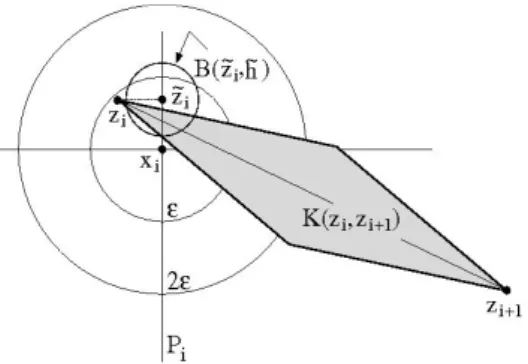
Proof.We follow [30, Prop. 5.2] with minor technical changes. Forx6=y∈R3we denote the closed halfspace
H+(x,y): ={z∈R3:hz−x,y−xi ≥0}. We shall work with ‘double cones’
K(x,y): =C1/4(x,y)∩C1/4(y,x)∩H+(x,y)∩H+(y,x).
For sake of brevity, set Ki:=K(xi,xi+1) andvi:=xi+1−xi. We are going to use Proposition4.1to verify two properties ofKi.
Claim 1.For each z∈Ki the intersection ofγand the two-dimensional disk Di(z):=Ki∩(z+v⊥i )
contains precisely one point. IfdiamDi(z)>0, then this point ofγis in the interior of Ki.
Indeed, note first thatγ∩Di(z)is nonempty, as an arc ofγjoiningxiwithxi+1must be contained inKisince if this were not the case, then (4.4) of Proposition4.1would be impossible for an injective and differentiableΓ. If there were two distinct pointsy1,y2∈γ∩Di(z), then (4.4) could not hold both for the couplex=xi,y=y1, and for the couple x=xi,y=y2, simultaneously. Finally, the second statement of Claim 1 follows from the fact that Inequality (4.1) is strict.
Claim 2.Whenever i6=j (modN)we find that the sets Ki\ {xi,xi+1}and Kj\ {xj,xj+1}are disjoint.
Suppose to the contrary that
(Ki\ {xi,xi+1})∩(Kj\ {xj,xj+1})6=/0, (5.20) and assume without loss of generality
diamKj≤diamKi. (5.21)
Ifxj=Γ(tj)were contained inKi\ {xi,xi+1}then we would either find that the diskDi(xj)contains two distinct curve points contradicting Claim 1, or that there is a parameter τ ∈(ti,ti+1) such that Γ(τ) =Γ(tj)althoughΓis injective, which is a contradiction. The same reasoning can be applied to xj+1=Γ(tj+1),so that we conclude from (4.4) and Assumptions (5.20) and (5.21) that the two tips xj,xj+1ofKj are contained in the setZidefined as
Zi:=C1
4(xi,xi+1)∩C1
4(xi+1,xi)∩B(xi,2|vi|)∩B(xi+1,2|vi|)\h
Ki\ {xi,xi+1}i
, (5.22)
which is just the intersection of the two cones within the balls centered inxi andxi+1but without the slab bounded by the two parallel planes∂H+(xi,xi+1)and∂H+(xi+1,xi).
We know thatxj 6=xisincei6=j (mod N)andΓis injective. Ifxj6=xi+1then (5.20), (5.21), and (5.22) enforce
|vi|(5.21)≥ |vj|(5.20)> min{|xj−xi+1|,|xj−xi|}, and
xj+1∈int(H+(xi,xi+1)) ∩ int(H+(xi+1,xi)), (5.23) which by (4.4) leads to xj+1 ∈Ki contradicting (5.22) unless xj+1=xi. If in the latter case xj is contained inR3\H+(xi+1,xi) then we obtain|vj|=|xj+1−xj|>|vi|contradicting our assumption (5.21). If, on the other hand,xjis inH+(xi+1,xi), it is by (5.22) actually contained inR3\H+(xi,xi+1), but then (5.20) cannot hold.
Finally,xj =xi+1 in combination with (5.20) also leading to (5.23) is a contradictory statement, since|vj| ≤ |vi|by (5.21).
We are now in the position to define the ambient isotopy betweenγandPγ. Note thatF:SL→R3 given by
F(t):= [xi,xi+1]∩Di(Γ(t)) for t∈[ti,ti+1),i=1, . . . ,N is a well defined homeomorphism, parametrizingPγ. The desired isotopy
H:R3×[0,1]→R3
is equal to the identity onR3\SNi=1Ki, and on each ‘double cone’Ki it maps each two-dimensional sliceDi(z),z∈Ki, homeomorphically to itself, keeping the boundary circle ofDi(z)fixed and moving the pointΓ(s)along a straight segment onDi(Γ(s))until it hits[xi,xi+1]. 2 Proof of Theorem1.2.Abbreviate the maximal energy valueE:=max{Eq(Γ1),Eq(Γ2)}of the two simple arclength parametrized curves Γi:SLi →R3 of respective (and a priori possibly quite differ- ent) lengths Li,i=1,2.Recall the assumption that the two curves are close in Hausdorff-distance:
distH(Γ1,Γ2)<δ(q)E−1(q−2).
FixN=N(q,E)so thatL1/N=:η<13δ2(q)E−1/(q−2), setε:=η/50 and letti:= (i−1)η∈SL1 fori=1, . . . ,N, andtN+1:=t1. By Proposition5.4,γ1is ambient isotopic to the polygonal line
Pγ1 :=
N
∑
i=1
[xi,xi+1]
wherexi:=Γ1(ti). Now, fori=1, . . . ,N we setwi:=Γ01(ti),αi:=Γ1 [ti,ti+1]
⊂γ1, and introduce the half-spacesHi+:=H+(xi,xi+wi)andHi−:=R3\Hi+, which are bounded by affine planesPi:=
xi+w⊥i . Consider the tubular regions
Ti:=Hi+∩Hi+1− ∩B35ε(αi).
Their union containsγ1=Sαi; we clearly haveTi∩Ti+1= /0 asαi+1⊂Hi+1+ . Moreover,Ti∩Tj= /0 also when|i−j|>1. To see this, we will use Proposition4.1to prove
inf{|Γ1(τ)−Γ1(σ)| : (σ,τ)∈SL1×SL1,|σ−τ| ≥η} ≥3 4η=3
4·50ε>35ε. (5.24) Before doing so, let us conclude from (5.24): If there existed a pointz∈Ti∩Tj with|i−j|>1, we could findσ∈[ti,ti+1)andτ∈[tj,tj+1)such that|Γ(σ)−Γ(τ)| ≤2ε=η/25 by triangle inequality, a contradiction to (5.24).
To verify (5.24), we repeat the trick that has already been used in the proof of Proposition5.2.
Notice that (4.3) applied toΓ1implies
|Γ1(τ)−Γ1(σ)| ≥ 3
4|τ−σ| ≥ 3
4η for all η≤ |τ−σ| ≤3η, (5.25) so that the continuously differentiable functiong:SL1×SL1 →Rgiven byg(s,t):=|Γ1(s)−Γ1(t)|2 attains a positive minimumg0>0 on the compact setK3η, where we setKρ:=SL1×SL1\{|s−t|<ρ}, i.e., there is a pair of parameters(s∗,t∗)∈K3η such thatg(s,t)≥g(s∗,t∗) =g0for all(s,t)∈K3η.If
|s∗−t∗|=3ηwe can apply (5.25) to find
|Γ1(τ)−Γ1(σ)|=p
g(τ,σ)≥p
g(s∗,t∗) =|Γ1(s∗)−Γ1(t∗)|(5.25)≥ 3
4η for all (τ,σ)∈K3η. If, on the other hand,|s∗−t∗|>3ηthen by minimality∇g(s∗,t∗) =0, which implies that both tangents Γ01(s∗)andΓ01(t∗)are perpendicular to the segmentΓ1(s∗)−Γ1(t∗).Thus the intersection
Γ1(SL1)∩B(Γ1(s∗),2√
g0)∩B(Γ1(t∗),2√ g0)
cannot be contained in the intersectionCφ(Γ1(s∗),Γ1(t∗))∩Cφ(Γ1(t∗),Γ1(s∗)),which according to (4.4) means that
|Γ1(s∗)−Γ1(t∗)| ≥δ2(q)Eq−2−1 >3η, establishing (5.24) also in this case.
Assume now that distH(γ1,γ2)<ε. We shall prove thatγ2is ambient isotopic toγ1; by the choice ofε, this will mean that Theorem1.2holds withδ3(q) =δ2(q)/150.
Claim. For each i=1, . . . ,N there is a point
yi∈Pi∩γ2∩B(xi,2ε).
Without loss of generality we can assume that the curveΓ1is oriented in such a way that
<)(Γ01(ti),vi)<1
8 and <)(Γ01(ti),vi−1)<1
8 for all i=1, . . . ,N, (5.26) that is, each tangent Γ01(ti) points into the set Ki :=K(xi,xi+1) =K(Γ1(ti),Γ1(ti+1)),which readily implies for the hyperplanesPi⊥Γ01(ti),i=1, . . . ,N,
<)(Pi,vi)≥<)(Pi,Γ01(ti))−<)(Γ01(ti),vi)>π 2−1
8, and similarly<)(Pi,vi−1)> π2−18.