Change point and trend analyses of annual expectile curves of tropical storms
Petra Burdejova
Wolfgang Karl Härdle
Piotr Kokoszka
Qian Xiong
Humboldt-Universität zu Berlin Unter den Linden 6
10099 Berlin
Tel: +49 30 2093-66336 Fax: +49 30 2093-66335 Web: www.iri-thesys.org
Author Contacts:
Petra Burdejova
IRI THESys, Humboldt-Universität zu Berlin, Unter den Linden 6, 10099 Berlin, Germany; C.A.S.E. - Center for Applied Statistics and Economics, Humboldt-Universität zu Berlin, Spandauer Str. 1, 10178 Berlin, Germany, E-mail: petra.burdejova@hu-berlin.de
Wolfgang Karl Härdle
IRI THESys, Humboldt-Universität zu Berlin, Unter den Linden 6, 10099 Berlin, Germany; C.A.S.E. - Center for Applied Statistics and Economics, Humboldt-Universität zu Berlin, Spandauer Str. 1, 10178 Berlin, Germany; Sim Kee Boon Institute for Financial Economics, Singapore Management University, 81 Victoria Street, Singapore 188065
Piotr Kokoszka
Department of Statistics, Colorado State University, 1877 campus delivery, Fort Collins, CO 80523, USA Qian Xiong
Department of Statistics, Colorado State University, 1877 campus delivery, Fort Collins, CO 80523, USA
Editor in Chief:
Jonas Østergaard Nielsen (IRI THESys) jonas.ostergaard.nielsen@hu-berlin.de
Cover:
West pacific typhoon intensity in year 2005 with expectile curves.
© Burdejova Petra, 2015
This publication may be reproduced in whole or in part and in any form for educational or non-profit purposes, without special permission from the copyright holder(s) provided acknowledgement of the source is made. No use of this publication may be made for resale or other commercial purpose, without written permission of the copyright holder(s).
Please cite as:
Burdejova, P., Härdle, W. K., Kokoszka, P., Xiong, Q. 2015. Change point and trend analyses of annual expectile curves of tropical storms. THESys Discussion Paper No. 2015-2. Humboldt-Universität zu Berlin, Berlin, Germany. Pp. 1-31.
edoc.hu-berlin.de/series/thesysdiscpapers
expectile curves of tropical storms ∗
P. Burdejova W. K. H¨ ardle P. Kokoszka Q. Xiong June 19, 2015
Abstract
Motivated by the conjectured existence of trends in the intensity of tropical storms, this paper proposes new inferential methodology to detect a trend in the an- nual pattern of environmental data. The new methodology can be applied to data which can be represented as annual curves which evolve from year to year. Other examples include annual temperature or log–precipitation curves at specific loca- tions. Within a framework of a functional regression model, we derive two tests of significance of the slope function, which can be viewed as the slope coefficient in the regression of the annual curves on year. One of the tests relies on a Monte Carlo distribution to compute the critical values, the other is pivotal with the chi–
square limit distribution. Full asymptotic justification of both tests is provided.
Their finite sample properties are investigated by a simulation study. Applied to tropical storm data, these tests show that there is a significant trend in the shape of the annual pattern of upper wind speed levels of hurricanes.
Keywords: change point, trend test, tropical storms, expectiles, functional data analysis
∗
Contents
1 Introduction 3
2 Change point and trend tests 4
2.1 Change point test . . . 5 2.2 Trend tests . . . 5
3 Application to typhoon and hurricane data 8
3.1 Change point analysis . . . 8 3.2 Trend analysis . . . 10 3.3 Main conclusions of data analysis . . . 13
A Construction of annual expectile curves 15
B Trend tests: finite sample performance 16
C Trend tests: large sample justification 19
C.1 Proof of Theorem 2.1 . . . 19 C.2 Proof of Theorem 2.2 . . . 24
References 29
1 Introduction
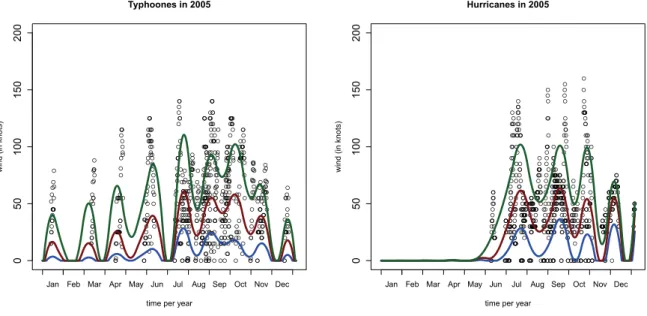
A great deal of research in environmental and climate sciences has been dedicated to detecting change points and trends in various time series, including those related to temperature, precipitation and wind speed. In a typical setting, a scalar time series X1, X2, . . . , XN is analyzed. Sometimes several correlated series are considered. Most environmental and climate series exhibit a pronounced annual periodicity which must be removed, or otherwise accounted for, before statements on change–points or trends can be inferred. Sometimes, it is difficult to approximate the periodic component by a Fourier expansion due to the irregular domain and amplitude of observations within a year. The data that motivate this work are tropical storm wind speed data, examples are shown in Figure 1. The onset and end of typhoon and hurricane seasons, as well as their intensity, can change from year to year. We therefore propose to treat the data avail- able for a whole year as a single high–dimensional data object and perform the change point and trend analyses on these objects rather than the scalar observations directly.
Such an approach is now relatively well–established in the field of functional data analy- sis (FDA), the monographs of Horv´ath and Kokoszka (2012) or Ferraty and Vieu (2006) contain many examples. Methodological foundations of FDA are addressed in Ramsay and Silverman (2005), its mathematical foundations in Hsing and Eubank (2015). While the amount of information available in the data is invariably reduced by various smoothing and dimension reduction methods, the most important and relevant features of the data come into focus. In the problems we study in this paper, we are interested in the evolu- tion of the annual pattern of tropical storms strength over several decades, not in specific hourly measurements.
Our functional methodology is combined with recent advances in expectile curve esti- mation, see Appendix A. We thus focus not only on the average pattern but on change points and trends in annual curves which describe the behavior at various levels of wind speed. This is illustrated in Figure 1. The curves in the middle summarize the pat- tern of average wind speed. These curves will exhibit some evolution from year to year.
The curves above them summarize the annual patterns of the highest speeds; they may exhibit a different evolution than the average curves. This issue is well–known in climate research; typically trends in the averages are contrasted with trends in extremes. In our application, no modeling of extreme behavior is required, the expectile curves are within the range of the data points. They provide information of behavior which lies between the typical behavior and the unobservable extreme behavior. Following the work of Smith (1989), evaluation of trends in extremes has attracted a great deal of attention, with re- spect to change point analysis of extremes, we are aware only of the work of Dierckx and Teugels (2010).
The data objects that this paper studies have the form Xn(t), where n refers to year, and t to time within the year. In the framework of functional data analysis, t is viewed as a continuous argument. The data are observed at a regular or irregular grid, but are converted to functional objects by means of various basis expansions which are defined for
●●
●
●
●
●
●
●
●
●
●
●●●
●
●
●
●
●
●
●
●
●
●●●
●
●
●
●
●
●
●
●
●
●
●
●
●
●
●
●●
●
●
●
●
●●●
●
●
●●
●
●
●
●
●
●
●
●
●
●
●●
●
●
●
●
●
●
●
●
●
●●●
●
●
●
●●
●
●
●
●
●
●●
●
●
●
●
●
●●
●
●
●●●
●
●
●
●
●●
●
●
●
●●●
●
●
●●
●
●
●
●
●●
●
●
●
●
●
●
●●
●
●●
●
●
●
●
●
●
●
●
●
●●
●
●
●●
●
●
●
●
●
●●
●
●
●●
●
●
●
●
●
●
●
●
●
●
●
●
●
●
●
●
●
●
●
●
●
●
●
●
●
●
●
●●
●
●
●
●
●
●
●
●
●
●
●
●
●
●
●
●
●
●●●
●
●
●●
●
●
●●
●
●●
●
●
●
●
●
●
●
●
●●
●
●
●
●
●
●
●
●
●
●
●
●
●
●
●
●
●
●
●
●
●●
●
●
●
●●
●
●
●
●
●
●
●
●
●●
●
●
●
●
●
●●
●
●
●
●
●
●
●
●
●
●●
●
●
●
●
●
●
●
●
●
●●●●
●
●
●
●
●●
●
●
●
●
●
●
●
●
●
●
●
●
●●
●
●
●
●
●
●
●
●
●
●
●
●
●
●
●
●
●
●
●
●
●
●
●
●
●
●
●
●
●
●
●
●
●
●
●
●
●
●
●
●
●
●
●
●
●
●
●
●
●
●
●
●
●
●
●
●
●
●
●
●
●
●
●
●
●
●
●
●
●
●
●
●
●
●
●
●
●
●
●
●
●
●
●
●
●
●●
●
●●
●
●
●
●
●
●
●
●
●
●
●
●●
●
●
●
●
●
●
●
●
●
●
●
●
●
●
●
●
●
●●
●
●
●
●
●
●
●●
●
●●●
●
●
●
●
●
●
●
●
●
●
●
●
●
●
●
●●
●
●
●
●
●
●
●
●●
●
●●
●
●
●
●
●
●
●●
●
●●
●
●
●●
●
●
●
●
●
●
●
●
●
●
●
●
●
●
●
●
●
●
●
●
●
●
●
●
●
●
●
●
●
●
●
●
●
●
●
●
●
●●
●
●
●
●
●
●
●
●
●
●
●
●●
●
●
●
●●
●
●
●
●●
●
●
●
●
●●●
●
●●●
●
●
●
●
●
●
●
●
●
●
●
●●
●
●
●●●●●
●
●
●
●
●
●
●●
●
●
●
●
●
●
●●●
●
●●
●
●
●
●
●
●●
●
●
●
●
●●
●
●
●
●
●
●
●
●
●
●
●
●
●
●
●
●
●
●●
●
●
●
●
●
●
●
●
●
●●●
●
●●
●
●
●
●
●
●
●●●
●
●
●●
●
●
●
●
●
●●
●
●
●●●
●
●
●●
●
●●
●
●
●
●
●
●
●●●
●
●
●●
●
●
●
●
●
●
Typhoones in 2005
time per year
wind (in knots)
Jan Feb Mar Apr May Jun Jul Aug Sep Oct Nov Dec
050100150200
●●●
●
●
●
●●●●●●●●
●
●
●
●●●●●●●
●
●●
●
●
●
●
●
●
●
●
●●●●
●
●
●
●
●
●
●
●
●
●
●
●
●
●
●
●
●
●
●
●
●
●
●
●
●
●
●
●
●
●
●
●
●
●
●
●
●
●
●
●
●
●
●●
●
●
●●●
●
●
●
●
●
●
●
●
●
●
●
●
●
●
●
●
●
●
●
●
●●
●
●
●
●
●
●
●
●
●
●●
●
●
●●
●
●
●
●
●
●
●
●
●
●
●
●
●
●
●
●
●
●
●
●
●●●●
●
●
●
●
●
●
●
●
●
●
●
●
●
●
●
●
●
●
●
●
●
●
●
●
●
●
●
●●●●●●
●
●
●
●
●
●
●
●
●
●
●
●●
●
●
●
●
●
●
●
●
●
●
●
●
●
●
●
●
●
●
●
●
●
●
●
●
●
●
●
●
●
●
●
●
●
●
●
●
●
●
●
●
●●●●●●●●●●●●●●
●
●
●●
●●●●
●
●●
●●
●
●
●●●●
●
●
●●
●
●
●
●●●
●
●
●
●
●
●
●
●
●
●
●
●
●●●●●●
●
●
●
●●
●
●●●
●
●
●
●
●
●
●
●
●
●
●
●
●
●
●
●
●
●
●●
●
●
●
●
●
●
●
●
●
●
●
●
●
●
●●
●
●
●●●●
●
●
●
●
●
●
●
●
●
●
●
●
●
●
●
●
●
●
●
●
●
●
●
●
●
●
●
●
●
●
●●
●
●●
●
●
●
●
●
●
●
●
●
●
●
●
●
●
●
●
●
●
●
●
●
●
●
●●
●
●
●
●
●
●
●
●
●●●
●
●
●
●●●●●●●●●●●●
●
●
●
●●
●●●
●
●
●
●
●
●
●
●
●
●
●
●
●
●
●
●
●
●
●
●
●
●
●
●
●
●
●
●
●
●
●
●
●
●
●
●
●
●
●
●
●
●
●
●
●
●
●
●
●
●
●
●
●
●
●●
●
●
●
●
●
●
●●
●
●
●●●
●
●
●
●
●●
●
●
●
●●
●
●
●
●
●
●
●
●
●
●
●
●
●
●
●
●
●●●
●
●
●
●
●●●
●●●●
●
●
●
●
●●●●●
●●●
●
●
●
●
●●
●
●
●
●●
●●
●
●
●
●
●
●
●
●
●
●
●
●
●
●
●
●
●
●
●
●
●
●
●
●
●
●
●
●
●
●
●
●●●
●
●
●
●●●
●
●●
●
●
●
●
●
●
●
●
●
●
●
●●●●●
●
●●
●
●
●
●
●
●
●
●
●
●
●
●
●
●
●
●
●
●
●
●●●●
●
●
●
●●
●
●
●
●
●●●●●●
●
●
●
●
●
●●
●
●
●
●
●●●●●●●●●●●●●●●●
●
●●●●●●●
●
●
●
●
● ●
●●●●●●
●
Hurricanes in 2005
time per year
wind (in knots)
Jan Feb Mar Apr May Jun Jul Aug Sep Oct Nov Dec
050100150200
Figure 1: Typhoons (left) and hurricanes (right) data in 2005 with expectile curves for
τ = 0.1,0.5 and 0.9. data load hurricanes.R
these are similar to quantile levels. We are interested in detecting change points and trends in the functional time series X1(·, τ), X2(·, τ), . . . , XN(·, τ). For this purpose, we use the existing change point test of Berkes et al. (2009) and develop two trend tests. No trend tests have presently been available for the data structure described above. These two tests form a methodological contribution to statistics, while the analysis of the expectile curves of tropical storms provides an insight to climate science.
The paper is organized as follows. In Section 2 we review the test of Berkes et al. (2009) and present the two trend tests. These tools are applied in Section 3 to the analysis of expectile curves. Three appendices contain, respectively, background on expectile curves, a simulation study, and the details of the asymptotic theory for the trend tests. All codes are available as Quantlets on Quantnet (2015).
2 Change point and trend tests
This section presents the significance tests that will be applied to tropical storm data in Section 3. The change point test described in Section 2.1 was derived by Berkes et al.
(2009), it is also described in Chapter 6 of Horv´ath and Kokoszka (2012). Trend tests introduced in Section 2.2 are new; their derivation and full large sample justification are presented in Section C. In both inferential settings, we consider as sequence of curves Xn(t), t ∈ [0,1], n = 1,2, . . . N. The index n can be identified with year, the index t with time within the year normalized to unit interval. The exposition that follows uses now fairly standard concepts of functional data analysis, including functional principal components (FPC’s) and their empirical counterparts (EFPC’s), see e.g. Chapter 3 of
Horv´ath and Kokoszka (2012).
2.1 Change point test
In change point tests, the null hypothesis is that the mean function does not change with year:
H0 : EX1 =EX2 =. . .=EXN.
The specific value of the mean is not part of the null hypothesis. The alternative is that there are change points k∗1, k2∗, . . . , kM∗ such that the means Xi are not the same in all segments (k∗m−1, k∗m]. The theory and practice of change points tests have been described in many textbooks, e.g. Brodsky and Darkhovsky (1993), Cs¨org˝o and Horv´ath (1997), Chen and Gupta (2011), so we do not dwell on the background on move on to the description of the test of Berkes et al. (2009).
The test is based on the normalized differences of estimated mean functions:
Pk(t, τ) = k(N −k)
N {μˆk(t, τ)−μ˜k(t, τ)}, where
ˆ
μk(t, τ) = k−1 k
i=1
Xi(t, τ), μ˜k(t, τ) = (N −k)−1 N i=k+1
Xi(t, τ).
Next, we compute the estimated functional principal components ˆv of the curvesXn and calculate the scores
ξˆj,n = 1
0
Xn(t)−X¯N(t) ˆ
vj(t)dt. (2.1)
The scores are calculated using the function pca.fd in the R package fda, see Chapter 7 of Ramsay et al. (2009). This function also produces estimated eigenvalues ˆλ and the percentage of variance explained by the first d eigenvalues. We find the smallest d such that 85% of the variance is explained and calculate the test statistic
Sd= 1 N2
d j=1
1 λˆj
N k=1
1≤i≤k
ξˆj,i− k N
1≤i≤k
ξˆj,i
.
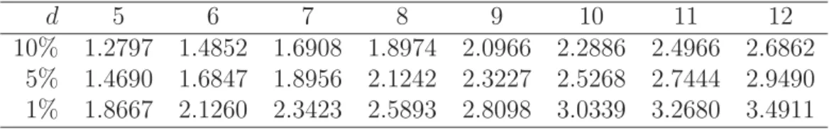
For large N, the statistics Sd has approximately the same distribution as the random variable Kd whose critical values are given Table 1, see Horv´ath and Kokoszka (2012) for more details.
2.2 Trend tests
Suppose the functions Xn(t) follow the trend model
d 5 6 7 8 9 10 11 12 10% 1.2797 1.4852 1.6908 1.8974 2.0966 2.2886 2.4966 2.6862
5% 1.4690 1.6847 1.8956 2.1242 2.3227 2.5268 2.7444 2.9490 1% 1.8667 2.1260 2.3423 2.5893 2.8098 3.0339 3.2680 3.4911
Table 1: Critical values of the distribution of Kd, which approximates the distribution of the statistic Sd for largeN.
in which the error functionsεnare iid and square integrable: E||εn||2 =E 01ε2n(t)dt < ∞. The testing problem in this setting is
H0 : β = 0, vs. HA: β = 0.
The parameter functions α, β are assumed to be elements of the spaceL2 =L2([0,1]), so technically, β = 0 means that β(t) = 0 for almost all t.
A natural approach to testing is based on an estimator of β. If this estimator is small for allt ∈[0,1], there is not enough evidence to rejectH0. The least squares estimator of β , cf. Section C, is given by
β(t) =ˆ 6
N(N + 1)(N −1) N
k=1
(2k−N −1)Xk(t). (2.3) Our first approach is based on the statistic 01βˆ2(t)dt. To describe its asymptotic dis- tribution additional notation is needed. Introduce the covariance function of the errors cε(t, s) = E[εn(t)εn(s)]. Denote by λj, j = 1,2, . . . the eigenvalues of cε. Next, define the residuals
ˆ
εn(t) =Xn(t)−αˆn(t)−βˆn(t)n, (2.4) where
ˆ
α(t) = 2 N(N −1)
N k=1
(2N + 1−3k)Xk(t). (2.5)
Denote by ˆλj the eigenvalues of the empirical covariance function ˆ
cε(t, s) = 1 N
N n=1
ˆ
εn(t)ˆεn(s). (2.6)
Theorem 2.1 describes large sample properties of the suitably normalized statistic
1
0 βˆ2(t)dt.
Theorem 2.1 (i) Under H0, ΛN = N3
12 1
0
β(t)ˆ 2
dt−→L Λ∞ def= ∞ j=1
λjZj2, (2.7)
where {Zj, j ≥1} are independent standard normal variables, and the λj are the eigen- values of the covariance function cε.
(ii) Under HA,
P
ΛN > qN(α)
→1, as N → ∞, (2.8)
where qN(α) is the (1−α)th quantile of the distribution of ΛN =N
j=1ˆλjZj2. Theorem 2.1 is proven in Section C.
The distribution of Λ∞ can be approximated by the distribution of ΛN =
N j=1
ˆλjZj2. (2.9)
This leads to the Monte Carlo test whose consistency is claimed in part (ii) of Theo- rem 2.1. To implement the test, we generate a large number, sayR= 104, of independent replications of ΛN (the ˆλj are estimated only once, from the original sample). Denote these replications by ΛN,r,1≤r ≤R. The P–value of the test is computed as the fraction of the ΛN,r which are greater than ΛN (computed from the data).
It is also possible to develop a test similar to the test of Berkes et al. (2009) in the sense that a limit distribution is independent of the distribution of the data. In fact, in the trend model, the limit distribution is the usual chi–square distribution. This is stated in Theorem 2.2, in which we use the inner product notation f, g= 01f(t)g(t)dt.
Theorem 2.2 Suppose E||ε||4 <∞ and
λ1 > λ2 > . . . > λq > λq+1 >0. (2.10) i) Under H0,
TN = N3 12
q j=1
λˆ−1j β,ˆ vˆj
2 L
−→χ2q. (2.11)
ii) If for some 1≤j ≤q, β, vj = 0, then the test is consistent, i.e.
P
TN > q(α)
→1, as N → ∞, (2.12)
whereq(α)is the(1−α)th quantile of the chi–square distribution withqdegrees of freedom.
Theorem 2.2 is proven in Section C.
Observe that to establish the consistency, it is not enough to assumeβ = 0 inL2. Since the statistic TN is based on projections on the first q EFPC’s, we must assume that the slope function β is not orthogonal to the subspace spanned by the first q FPC’s.
3 Application to typhoon and hurricane data
In this section we apply the tests of Section 2 to annual expectile curves of wind speed data. The data have the form Xn(ti), where the timesti are separated by six hours, and the index n stands for year. The value Xn(ti) is the wind speed in knots (1 kn = 0.5144 m/s). We work with two data sets: typhoons in the West Pacific area over the period 1946–2010, and hurricanes across the North Atlantic basin over the period 1947-2011.
Both datasets are accessible free of charge at the website of Unisys Weather Information, UNISYS (2015).
Since there are about 1,460 time points ti per year, we treat time 0 ≤ t ≤ T within a year as continuous, and the observed curves as functional data. For each year n, we construct expectile curves Xn(t, τ), forτ = 0.1,0.2, . . . ,0.9. Examples of expectile curves we study are given in Figure 1. The index τ ∈ (0,1) has the following interpretation. If τ = 0.5, the curve Xn(t, τ) describes the median strength of tropical storms throughout the year. Ifτ is close to 1, the curveXn(t, τ) captures the annual pattern of highest wind speeds. Ifτ is close to zero, it does the same for the lowest wind speeds. More details are provided in Appendix A.
3.1 Change point analysis
The results of the application of the change–point test of Section 2.1 are shown in Table 2.
For both data sets and at all levels τ, the test rejects the null hypothesis that the mean pattern does not change. As explained in Appendix A, the construction of the expectile curves involves the selection of a smoothing parameter λ. Table 2 shows the results for λ selected by the AIC criterion. To validate our conclusions, we performed the same analysis using λ which is either twice or half of theλ selected by AIC. In both cases, all empirical significance levels remained under 5%.
τ 0.1 0.2 0.3 0.4 0.5 0.6 0.7 0.8 0.9
d 10 11 12 12 12 12 12 12 12
Sd 3.3522 3.2291 3.4317 3.4978 3.6564 3.8554 4.0342 4.2317 4.5084
*** ** ** *** *** *** *** *** ***
τ 0.1 0.2 0.3 0.4 0.5 0.6 0.7 0.8 0.9
d 5 5 5 6 6 6 7 7 7
Sd 2.7440 3.3993 3.8759 4.4640 4.7141 4.8680 5.0366 4.9247 4.5740
*** *** *** *** *** *** *** *** ***
Table 2: Results of the application of the change point test of Section 2.1 to typhoon (upper panel) and hurricane (lower panel) expectile curves. Usual significance codes are used: ** – significant at 5% level, *** - at 1% level.
The change point test shows that for all expectile levels τ, there are statistically signif- icant changes in the annual pattern. It is instructive to complement the above inferential analysis by simple exploratory analysis that reveals some dependence on the level τ.
0 10 20 30 40 50 60
5.0e+061.0e+071.5e+07
τ =0.9 τ =0.5 τ =0.1
0 10 20 30 40 50 60
0e+004e+068e+06
Figure 2: The squared norms Pn(τ) showing the magnitude of change in mean annual pattern for expectile curves of typhoons (upper panel) and hurricanes (lower panel).
The largest changes occur in the expectile curves corresponding to τ = 0.9.
P beta est.R Consider squared norms
Pn(τ) = T
0
Pn2(t, τ)dt
of the normalized differences introduced in Section 2.1. The plot ofPn(τ) against the year index n shows the magnitude of change of the mean function. We display such plots in Figure 2. They suggest that the largest changes occur for the expectile levels τ close to one, but it must be kept in mind that they may just reflect the fact that the curvesXn(t) are ”larger” for larger τ. By contract, the statistic Sd contains a normalization with the variances ˆλj, and is scale invariant.
The change point analysis above shows that the pattern of typhoon and hurricane wind speeds cannot be treated as stable over the sample periods we study. In the next section, we investigate if this instability can be attributed to systematic trends.
3.2 Trend analysis
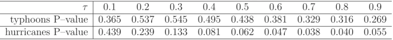
We now apply the trend tests introduced in Section 2.2 to typhoon and hurricane expec- tile curves. In the Monte Carlo test based on Theorem 2.1, we use 104 replications of the random variable ΛN defined by (2.9). In the chi–square test based on Theorem 2.2, we determine q as the smallest number which explains at least 85% of the variance of the residual curves ˆεn defined by (2.4). The results of the tests are presented in Tables 3 and 4.
τ 0.1 0.2 0.3 0.4 0.5 0.6 0.7 0.8 0.9
typhoons P–value 0.365 0.537 0.545 0.495 0.438 0.381 0.329 0.316 0.269 hurricanes P–value 0.439 0.239 0.133 0.081 0.062 0.047 0.038 0.040 0.055
Table 3: P–values for the Monte Carlo trend test based on Theorem 2.1
τ 0.1 0.2 0.3 0.4 0.5 0.6 0.7 0.8 0.9
q 10 11 12 12 12 12 12 12 12
typhoons P–value 0.534 0.705 0.722 0.688 0.587 0.466 0.382 0.371 0.453
q 5 5 5 6 6 6 7 7 7
hurricanes P–value 0.069 0.024 0.015 0.006 0.003 0.003 0.004 0.006 0.035 Table 4: P–values for the chi–square trend test based on Theorem 2.2
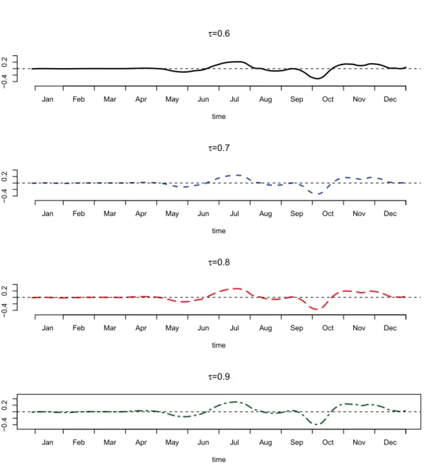
For the typhoon data, none of the two tests finds evidence of a trend. For the Hurricane data, the Monte Carlo test based on Theorem 2.1 indicates the existence of a trend for expectile levels τ = 0.6−0.9 while the chi–square test of Theorem 2.2 for all τ except τ = 0.1. Simulations reported in Appendix B show that the chi–square test tends to overreject for data generating processes (DGP’s) of length and error structure similar to the tropical storm expectile curves. We therefore conclude that there is evidence for the existence of a trend for upper expectile functions of hurricane data. The estimated slope functions ˆβ are plotted in Figure 3.
We conclude the trend analysis by showing in Figure 5 the dependence onτ of the norm βˆ = βˆ2(t)dt of the estimated slope function. Even though there is statistical evi- dence for nonzero slope function only for the upper expectiles of hurricane data, the ex- ploratory analysis of the norms indicates that there is a very clear increasing dependence of the slope on τ. Again, the increasing norms could be attributed to the increasing size of the curve Xn(t), and the plots can be used only as an exploratory tool for comparing the hurricane and typhoon data.
There is not much difference between the size of ˆβ, for typhoon and hurricane data, but the ˆβ for hurricanes show a clear pattern with positive mass around July and November, and negative mass in early Fall. For the typhoon curves the pattern of mass accumula- tion is spread more uniformly throughout the year, with a pronounced negative mass in November. The significance tests we developed provide a statistical justification for these fairly subtle visual differences.
τ=0.6
time
Jan Feb Mar Apr May Jun Jul Aug Sep Oct Nov Dec
−0.40.2
τ=0.7
time
Jan Feb Mar Apr May Jun Jul Aug Sep Oct Nov Dec
−0.40.2
τ=0.8
time
Jan Feb Mar Apr May Jun Jul Aug Sep Oct Nov Dec
−0.40.2
τ=0.9
time
Jan Feb Mar Apr May Jun Jul Aug Sep Oct Nov Dec
−0.40.2
Figure 3: Estimated slope functions, ˆβ, for upper expectile curves of hurricane data.
P beta est.R
τ=0.6
time
Jan Feb Mar Apr May Jun Jul Aug Sep Oct Nov Dec
−0.40.2
τ=0.7
time
Jan Feb Mar Apr May Jun Jul Aug Sep Oct Nov Dec
−0.40.2
τ=0.8
time
Jan Feb Mar Apr May Jun Jul Aug Sep Oct Nov Dec
−0.40.2
τ=0.9
time
Jan Feb Mar Apr May Jun Jul Aug Sep Oct Nov Dec
−0.40.2
Figure 4: Estimated slope functions, ˆβ, for upper expectile curves oftyphoon data.
●
●
●
●
●
●
●
●
●
Typhoons
0.000.050.100.150.20
0.1 0.2 0.3 0.4 0.5 0.6 0.7 0.8 0.9
●
●
●
●
●
●
●
●
●
Hurricanes
0.000.050.100.150.20
0.1 0.2 0.3 0.4 0.5 0.6 0.7 0.8 0.9
Figure 5: Norm of the slope function estimate, ˆβ, as a function of the expectile level τ;
typhoons (left), hurricanes (right). P beta est.R
3.3 Main conclusions of data analysis
The change point tests have shown that the annual pattern of wind speeds for both hurricanes and typhoons cannot be treated as constant, no matter what expectile level is considered. The application of the new trend tests has focused on a more subtle question, which has however received a fair deal of attention: is there a trend in the intensity of tropical storms. A review of relevant research is not our aim, the paper of Kossin et al.
(2013) provides background and references. There are two novel aspects to our approach:
1) focus on the annual curves, 2) separate analysis for each intensity level. Based on sixty years of data, our tests detect a trend in the upper wind speeds of Atlantic hurricanes.
Exploratory analysis suggests a similar conclusion for Pacific typhoons, but it cannot be supported by low P–values with the amount of available data. These conclusions are similar to the findings of Kossin et al. (2013) who use different, custom–prepared, data sets. Their P–value for the existence of a trend in North Atlantic is less that 10−3, but for the North–West pacific it is 0.03 (for South Pacific it is 0.09, 0.06 for the South Indian Ocean). Their analysis is concerned with the trend in the scalar data, not a trend in the annual pattern. They find all trends to be positive. In a sense, such trend coefficients can be viewed as averages of the annual curves like those displayed in Figures 3 and 4.
The hurricane curves indeed have more positive mass, whereas for the typhoon curves the negative mass is larger (the typhoon curves are not statistically different from zero, according to our tests). The slope functions of the hurricanes indicate increasing intensity in summer and late fall, and decreasing intensity in early fall. For typhoons, these curves indicate decreasing intensity in November.
The conclusions of this paper which are supported by significance tests and do not contradict existing research are as follows:
ing at all wind speed levels over the last 60 years.
2. There is a significant trend in the shape of this pattern for upper wind speed levels of hurricanes.