as Order Matrices:
Basic Concepts, Formal Properties, Algorithms
Chen Li1 ?, Manfred Reichert2, and Andreas Wombacher3
1 Information Systems Group, University of Twente, The Netherlands lic@cs.utwente.nl
2 Institute of Databases and Information Systems, Ulm University, Germany manfred.reichert@uni-ulm.de
3 Database Group, University of Twente, The Netherlands a.wombacher@utwente.nl
Abstract. In various cases we need to transform a process model into a matrix representation for further analysis. In this paper, we introduce the notion of Order Matrix, which enables unique representation of block- structured process models. We present algorithms for transforming a block-structured process model into a corresponding order matrix and vice verse. We then prove that such order matrix constitutes a unique representation of a block-structured process model; i.e., if we transform a process model into an order matrix, and then transform this matrix back into a process model, the two process models are trace equivalent;
i.e., they show same behavior. Finally, we analyze algebraic properties of order matrices.
1 Introduction
In various cases we need to transform a process model into a matrix represen- tation for further analysis. For example, in graph theory adjacency matrices are often used for various kinds of graph analysis (e.g., reachability analysis or derivation of minimal spanning tree [25]). In process mining,causal matricesare used to represent the relationship between transitions in Petri nets. Causal ma- trices are further applied in genetic process mining to discover a process model which covers the execution traces of a collection of process instances best [7]. In the field of data mining, matrices are used to classify, cluster or associate data [26, 20]. However, all these techniques are focusing on the nodes and edges of a graph or process model, and cannot be applied in respect to the management of process changes [12].
In this paper, we introduce the notion oforder matrix, which represents all transitive relations between the activities of a block-structured process model.
In the context of managing process variants [8], for example, we have already
?This work was done in the MinAdept project, which has been supported by the Netherlands Organization for Scientific Research under contract number 612.066.512.
applied this kind of matrix for measuring the structural similarity between two process models [13]. We have further used order matrices for mining structurally different process variants. Here, we aim at discovering a process model that structurally covers a collection of process variants best [11, 14]. The present paper focuses on basic concepts, algorithms and formal properties of order matrices, and less on their use.
The remainder of this paper is organized as follows: Section 2 introduces some basic definitions needed for understanding this paper. Section 3 then provides the formal definition of an order matrix and gives an illustrative example. Section 4 presents an algorithm for transforming a block-structured process model into an order matrix. Section 5 presents an algorithm for transforming an order matrix back into a block-structured process model. In Section 6, we prove that there exists a one-to-one mapping between a process model and its order matrix, i.e., if one transforms a process model into an order matrix, and then transform this matrix back into a process model, the two models will be same. Finally, we present algebraic properties of order matrices in Section 7.
2 Backgrounds
We first introduce basic notions needed in the following:
Process Model: Let P denote the set of all sound (i.e., correct) process models. We denote a process model as sound if there are no deadlocks or un- reachable activities in the process model [21, 28]. In our context, a particular process model S = (N, E, . . .)4 ∈ P is defined in terms of an Activity Net [21].
N constitutes the set of activities andEthe set of control edges (i.e., precedence relations) linking them. More precisely, Activity Nets cover the following funda- mental process patterns: Sequence, AND-split, AND-join, XOR-split, XOR-join, and Loop [27].5These patterns constitute the core set of any workflow specifica- tion language (e.g., WS-BPEL [3] and BPMN [4]) and cover most of the process models we can find in practice [36, 15]. Furthermore, based on these patterns we are able to compose more complex ones if required (e.g., an OR-split can be mapped to XOR- and AND- splits [19]). Finally, when restricting process modeling to these basic process patterns, we obtain models that are better un- derstandable and less erroneous [18, 16]. A simple example of an Activity Net is depicted in Fig. 1a. For a detailed description and correctness issues we refer to [21].
Block Structuring: To limit the scope, we assume Activity Nets to be block-structured, i.e., sequences, branchings (with aforementioned split and join semantics), and loops are specified as blocks with well-defined start and end nodes. These blocks may be nested, but must not overlap, i.e., the nesting must
4 A Well-structured Activity Net contains more elements than only node set N and edge setE, which can be ignored in the context of this paper.
5 These patterns can be mapped to other languages as well. For example in Business Process Execution Language (BPEL), XOR-Split / -join can be represented by ’If’
or ’Pick’, AND-Split / -Join by ’Flow’, and Loops by ’While’ or ’RepeatUntil’ [3].
be regular [21, 10]. A block in a process model S can be a single activity, a self-contained part of S, or even S itself. As example consider process model S from Fig. 1. Here {A}, {A,B}, {C,F}, and {A,B,C,D,E,F,G} describe pos- sible blocks contained in S. Note that we can represent a block B as activ- ity set, since the block structure itself already becomes clear from the process modelS. For example, block{A,B}corresponds to the parallel block with corre- sponding AND-split and AND-join nodes inS. The concept of block-structuring can be found in languages like WS-BPEL [3]. When compared with non-block- structured process models, block-structured ones are easier understandable for users and have less chances of containing errors [23, 16–18]. If a process model is not block-structured, in most practically relevant cases we can transform it into a block-structured one (see [31, 18, 10]).
Definition 1 (Trace). Let S = (N, E, . . .)∈ P be a process model. We define t as a trace ofS iff:
– t ≡< a1, a2, . . . , ak > (with ai ∈N) constitutes a valid and complete exe- cution sequence of activities considering the control flow defined byS. We define TS as the set of all traces that can be produced by process instances running on process modelS.
– t(a≺b) is denoted as precedence relationship between activities a and b in tracet≡< a1, a2, . . . , ak>iff∃i < j :ai=a∧aj =b.
We only consider traces composing ’real’ activities, but no events related to silent activities, i.e., nodes in a process model having no associated action and only existing for control flow purpose [13]. At this stage, we consider two process models as being the same if they are trace equivalent, i.e., S ≡ S0 iff TS ≡ TS0. Like most process mining approaches [30, 7, 34], the stronger notion of bi-similarity [9] is not considered in our context.
3 Basic Definition of an Order Matrix
One key feature of our ADEPT change framework is to maintain the struc- ture of the unchanged parts of a process model [21, 6, 33]. For example, when deleting an activity this neither influences successors nor predecessors of this activity, and therefore also not their order relations [24, 22]. To incorporate this feature in our approach, rather than only looking at direct predecessor-successor relationships between activities (i.e. control edges), we consider the transitive control dependencies for each pair of activities; i.e., for a given process model S= (N, E, . . .)∈ P, for activitiesai, aj∈N,ai6=ajwe examine their structural order relations (including transitive order relations). Logically, we determine or- der relations by considering all traces in trace setTS producible by modelS.
Fig. 1a shows an example of a process modelS. This model comprises process patterns like Sequence, AND-block, XOR-block, and Loop-block [27]. Here, trace setTS ofSconstitutes an infinite set due to the presence of the loop-block inS (cf. Fig. 1b). Such infinite number of traces precludes us to perform any detailed analysis of the trace set. Therefore we need to transform such infinite trace sets into a finite representation for further analysis.
3.1 Simplification of Infinite Trace Sets
One common approach to represent a string with infinite length is to represent it as finite set of n-gram lists [5]. The general idea behind an n-gram list is to represent a single string by an ordered list of substrings with lengthn(so-called n-grams). In particular, only the first occurrence of an n-gram is considered, while later occurrences of the same n-gram are omitted in the n-gram list. Thus, an n-gram list represents a collection of strings with different length. In particular, an infinite language can be represented as finite set of n-gram lists. For example, a string < abababab > can be represented as 2-gram <$a, ab, ba, b# >, where
$ (#) represents the start (end) of the string. Such approach is commonly used for analyzing loop structures in process models [35, 2], or - more generally - in the context of text indexing for substring matching [1]. Inspired by the n-gram approach, we define the notion ofSimplified Trace Set as follows:
Definition 2 (Simplified Trace Set).
LetSbe a process model andTS denote the trace set producible onS. LetBk, k= (1, . . . , K)be Loop-blocks inS, andTBk denote the set of traces producible on Bk. Let further(tBk)m be a sequence ofm (m∈N) traces< t1Bk, t2Bk, . . . , tmBk>
with tjB
k ∈ TBk, j ∈ {1, . . . , m}. We additionally define (tBk)0 =<> as an empty sequence. If we only consider the activities corresponding to Bk, in any trace t ∈ TS producible on S, t either has no entries 6 or must have structure
< t∗Bk,(tBk)m>, witht∗Bk∈ TBkrepresenting the first loop iteration andm∈N0
being the number of additional iterations loop-block Bk is executed in trace t.
We can simplify this structure by using < tBk, τk >instead, whereτk refers to (tBk)m. When simplifying trace set TS this way, we obtain a finite set of traces TS0, denoted as Simplified Trace Setof process modelS.
In our representation of a tracet∈ TS, we only consider the first occurrence of tracet∗B
kproducible by blockBkwhile omitting others that occur later within tracet. Instead, we represent such repetitive entries by a silent activityτk, which has not associated action but solely exists to indicate omission of other tBk
appearing later in tracet, i.e.,τk represents the iterative execution of loop-block Bk captured in tracet.7 When omitting repetitive entries within trace set TS, we obtain a finite trace set TS0 that we can use for further analysis. Note that when dealing with nested loops (e.g., a loop-block Bk contains another loop- block Bj), we first need to analyzeBj and thenBk; i.e., we need to first define τj to represent the iterative execution of loop-block Bj as captured in tracet and then defineτk to represent loop-blockBk.
As example consider process model S in Fig. 1a. Loop-block B, which is surrounded by a loop-backward edge, is the block comprising activities C and
6 i.e., the loop-blockBk has not been executed at all.
7 Though this approach is inspired by n-gram, it is different from n-gram representa- tion of a string. In n-gram the length of the sub-string is a fixed number n, while in our approach we use τk to represent traces producible by the Loop-block Bk. Obviously, traces producible byBk do not necessarily have same length.
Order matrix A Process model S
AND-Split AND-Join
XOR-Split XOR-Join
Control Flow Loop
A A B
B C D E F G
C D E F G
1
1 1 1 1
1 1 1 1 1
1 1
1 1 1 1
1 1
0 0 0
0 0
0 0 0
0 0
0 0
0 0
0 0 0 0
+ +
-
- -
- τ
τ
1 1
1 -
0 1
0 0 L 0 - L
L
L
‘0’ : successor ‘1’ : predecessor
‘+’ : AND-block ‘-’ : XOR-block
‘L’ : Loop
<A,B,D,E,G>;
<B,A,D,E,G>;
<A,B,D,C,F,τ,G>;
<B,A,D,C,F,τ,G>
S
A C
B E
F
D G
Trace set S
Simplified trace set S
<A,B,D,E,G>;
<B,A,D,E,G>;
<A,B,D,C,F,G>;
<B,A,D,C,F,G>;
<A,B,D,C,F,C,F,G>;
<B,A,D,C,F,C,F,C,F,G>;
……
S
(a) (b) (c)
Fig. 1.a) Process model and b) related order matrix
F; consequently the trace set this block can produce is {< C,F >}. Therefore, any trace t∈ TS producible onS has structure <C,F,(C,F)m>with m∈N0
depending on the number of times the loop iterates. For example, < C,F >,
< C,F,C,F > and < C,F,C,F,C,F > are all valid traces producible by the loop-block. Let us define a silent activity τ corresponding to block B. Then we can simplify these traces by <C,F, τ > where τ refers the to the sequence of the traces producible on B. This way, we can simplify infinite trace set TS
to finite set TS0 = {< A,B,D,E,G >, < B,A,D,E,G >, < A,B,D,C,F,τ,G >, <
B,A,D,C,F,τ,G>} (cf. Fig. 1b).
3.2 Defining an Order Matrix
For process modelS, the analyzing results of its trace set TS are aggregated in an order matrix A, which considers five types of order relations (cf. Def. 3):
Definition 3 (Order matrix). Let S = (N, E, . . .) ∈ P be a process model with activity setN ={a1, a2, . . . , an}. Let furtherTS denote the set of all traces producible on S and letTS0 be the simplified trace set ofS (cf. Def. 2). Let Bk, k = (1, . . . , K) denote loop-blocks in S. For every Bk, we define silent activity τk, k = (1, . . . , K) to represent the iterative structure producible by Bk in TS0. Then:
A is called order matrix of S with Aaiaj representing the order relation between activitiesai,aj∈NS
{tk
¯¯k= 1, . . . , K},i6=j iff:
– Aaiaj = ’1’ iff (∀t∈ TS0 withai, aj ∈t ⇒t(ai≺aj))
If for all traces containing activitiesai andaj,ai always appears BEFORE aj, we denoteAaiaj as ’1’, i.e.,aialways precedes ofajin the flow of control.
– Aaiaj = ’0’ iff (∀t∈ TS0 withai, aj ∈t ⇒t(aj≺ai))
If for all traces containing activities ai andaj, ai always appears AFTER aj, we denote Aaiaj as a ’0’, i.e. ai always succeeds of aj in the flow of control.
– Aaiaj = ’+’ iff (∃t1 ∈ TS0, with ai, aj ∈t1∧t1(ai ≺aj)) ∧(∃t2 ∈ TS0, with ai, aj∈t2∧t2(aj≺ai))
If there exists at least one trace in which ai appears before aj and another trace in whichai appears afteraj, we denoteAaiaj as ’+’, i.e.ai andaj are contained in different parallel branches.
– Aaiaj = ’-’ iff (¬∃t∈ TS0 :ai ∈t∧aj∈t)
If there is no trace containing both activityaiandaj, we denoteAaiaj as ’-’, i.e.ai andaj are contained in different branches of a conditional branching.
– Aaiaj = ’L’, iff ((ai∈Bk∧aj=τk)∨(aj∈Bk∧ai=τk))
For any activityaiin a Loop-blockBk, we define order relationAaiτk between it and the corresponding silent activityτk as ’L’.
The first four order relations{1,0,+,-} specify the precedence relations be- tween activities as captured in the trace set, while the last order relation ’L’
indicates loop structures within the trace set. Fig. 1c presents the order ma- trix of process model S. Since S contains one Loop-block, a silent activity τ is also added to this matrix. This order matrix contains all five order relations as described in Definition 3. For example, activities Eand C will never appear in same trace belonging to the simplified trace set since they are contained in different branches of an XOR block. Therefore, we assign ’-’ to matrix element AEC. Further, since in all traces which contain both activitiesBandG,Balways appears beforeG, we can obtain order relationABG= ’1’ and order relationAGB
= ’0’. Special attention should be paid to the order relations between the silent activity τ and the other activities. The order relation betweenτ and activities CandFis set to ’L’, since bothCandFare contained in the Loop-block; for all remaining activities, τ has same order relations with them as activities C or F have. Note that the main diagonal of the order matrix is empty, since we do not compare an activity with itself.
As one can see, elementsAaiaj andAajai can be derived from each other. If activityaiis a predecessor of activityaj, (i.e.Aaiaj = 1), we can always conclude that Aajai = 0 holds and ifAaiaj ∈ {’+’,’-’, ’L’}, we obtainAajai=Aaiaj.
4 Transforming a Process Model into an Order Matrix
Clearly, it is not realistic to first enumerate all traces of a process model and analyze the order relation based on them. The trace set of a process model can be extremely large particularly if the model contains several AND-blocks or even infinite if there are loop-blocks. In the following, we introduce Algorithm 1 to compute the order matrix for a process model in polynomial time. Note that this algorithm is also able to cope with loop structures.
In Algorithm 1, we first define set P(ai) for each activity ai ∈ N, which contains all (direct and indirect) predecessors of ai (Line 1). An activity aj is
input : A process modelS= (N, E, . . .) output: Its order matrixA
For each activityai∈N, i= (1, . . . , n), defineP(ai) as the predecessor set ofai;
1
Define SetCas the set of activities which are already parsed;
2
DefineLas the set of Loop-blocksBk;
3
P(ai) =∅fori= (1, . . . , n),C=∅andL=∅ /* initial state */;
4
SetparseModel(Nodetstart, Nodetend, SetC) begin
5
/* Compute predecessor sets for activities between node tstart and
tend. Returns a new C’ */
while(tstart6=tend)do
6
if (Sequence)then
7
P(tstart) =P(tstart).addAll(C) ;
8
C0=C.add(tstart) ;
9
tstart=tstart.nextNode;
10
else if (XOR-block)then
11
foreachbranchiin XOR-split,i= (1, . . . , m)do
12
ni= XOR-split.nextNodein branchi;
13
C0i =parseModel(ni, XOR-join,C) ;
14
C0=C.addAll(Sm
i=1C0i) ;
15
tstart= XOR-join.nextNode;
16
else if (AND-block)then
17
foreachbranchiin AND-split,i= (1, . . . , m)do
18
ni= XOR-split.nextNodein branchi;
19
C0i =parseModel(ni, XOR-join,C) ;
20
foreachbranchkin AND-split,k= (1, . . . , m)do
21
Ck=Sm
i=1,i6=kC0i;
22
parseModel(AND-split, AND-join,Ck);
23
C0=C.addAll(Sm
i=1C0i) ;
24
tstart= AND-join.nextNode;
25
else if (Loop-block)then
26
L.add(parseModel(Loop-start.nextNode, Loop-end,∅)) ;
27
C’ =C.addAll(parseModel(Loop-start,Loop-end,C)) ;
28
tstart= Loop-end.nextNode;
29
returnC0 ;
30
end
31
computeOrderRelationBasedOnPredecessorSets() begin
32
/* Compute order relation based on predecessor sets */; foreachai, aj∈N, i6=jdo
33
if P(ai)contain(aj)∧ ¬P(ai)contain(aj)then Aij= ’1’;
34
else if ¬P(ai)contain(aj) ∧P(ai)contain(aj)then Aij = ’0’;
35
else if P(ai)contain(aj)∧ P(ai)contain(aj)then Aij= ’+’;
36
else if ¬P(ai)contain(aj) ∧ ¬P(ai)contain(aj)then Aij = ’-’;
37
end
38
addSilentActivitiesForLoopStructure(SetL, OrderMatrixA) begin
39
/* Add loop on order matrix */;
foreachBk∈ Ldo
40
Define silent activityτk;N =N0S {τk};
41
foreachai∈N0do
42
if (ai∈Bk)then
43
Aaiτk = ’l’ ;Aτkai = ’l’ ;
44
else if (ai∈N0\Li)then
45
Letaj∈Li;
46
Aaiτk =Aaiaj ;Aτkai =Aajai ;
47
end
48
Algorithm 1: Computing order matrix for process model
a predecessor of ai iff∃t∈ TS0 : t(aj ≺ai). In addition, we define set L which contains all Loop-blocksBkof the process model. Following that, three functions are specified. FunctionparseModel(Lines 5 to 31) first parses the process model S and computes the predecessor setsP(ai) for each activity of the model. Fur- ther, it determines setLwhich contains all Loop-blocksBk ofS. Then function computeOrderRelationBasedOnPredecessorSets(lines 32 to 38) calculates the order relations for every pair of activities of modelSbased on their predecessor sets. Finally, functionaddSilentActivitiesForLoopStructure(lines 39 to 48) specially handles the loop structures of process modelS.
FunctionparseModelhas three input parameters: Nodeststartandtendmark the start and the end of the blockBi we need to analyze; setCcorresponds to the set of activities already been analyzed. After computing predecessor sets and Loop-blocks for the activities from block Bi, we obtain new set C’comprising original setCand all activities ofBi. Initially,tstartis set to the start-flow ofS, tend to the end-flow ofS, andCto an empty set (Line 5).
In our analysis, we consider four process patterns:
– Sequence. This pattern is analyzed in Lines 7 to 10 in Algorithm 1. Assume that blocksBi, Bj and Bk are three blocks of process model S, where Bi
precedesBj and Bj precedes Bk. Letai ∈Bi and aj ∈ Bj. For any trace t∈ TS containing bothaiandaj, we obtain t(ai≺aj). Therefore, for every aj ∈Bj, we need to addBi to its predecessor setP(aj). Similarly, for every ak ∈Bk, we need to add both Bi and Bj to its predecessor set P(ak). In Algorithm 1, we first addBi to setC, and then addCto everyP(aj)∈Bj. Finally we addBjtoC(lines 7-9). We repeat same procedure when analyzing Bk, i.e., we add Cto everyP(ak) withak∈Bk, and then addBk toC.
– XOR-block. This pattern is analyzed in Lines 10 - 15 in Algorithm 1. Since the activities in one branch of an XOR-block can never appear in tracet together with activities of another branch of same XOR-block, we analyze each branch of an XOR-block separately. Every branch i is considered as block ofS, which can be analyzed independently by the parseModel func- tion. In this case,tstart shall point to the first node on branchiandtend to the XOR-join node. Further we need to use same set C for analyzing each branchiin the XOR-block (line 14). This way, we can ensure that activities from a particular branch do not appear in the predecessor sets of activities from another branch of the XOR-block. After every branch is analyzed, we add all activities of this XOR-block to new setC’(Line 15).
– AND-block. This pattern is analyzed in Lines 17 - 25 of Algorithm 1. Sim- ilarly to XOR-blocks, we analyze each branch of an AND-block separately.
For every branchi, tstart shall point to the first node in branchi andtend
to the AND-join node. Further we use same setCfor every branch iin the AND-block (Line 20). Obviously, an AND-block differs from an XOR-block, since all its branches are executed concurrently. Therefore, for two activities ai and aj from two different branches in such AND-block, ai can appear beforeaj in one trace but appear afteraj in another trace. LetBAN D rep- resents the AND-block, and BiAN D be the block representing branch i of
BAN D. As reflecting on the predecessor setP(ai) for each ai ∈BiAN D, we need to add all activities from other branchesBAN D\BiAN D to its prede- cessor set. In Algorithm 1, Line 22 computes setBAN D\BAN Di and Line 23 adds them to the predecessors setsP(ai),ai ∈BiAN D. This way, we can ensure that two activities from different branches of an AND-block always appear in the predecessor sets of each other.
– Loop-block. This pattern is analyzed in Lines 26 - 29 in Algorithm 1.
We first determine which activities are contained in Loop-blockB by call- ing function parseModel and adding B to set L (Line 27). Then, we con- tinue parsing the model using function parseModel to analyze the activi- ties inside this Loop-block (Line 28). Note that the analysis of the prede- cessor sets is based on the simplified trace set (cf. Def. 2), i.e., we only consider the first appearance of trace tB ∈ TB producible by block B, while later appearances of tB (caused by the iterative executions of this Loop-block) are not considered any longer. It will handled later by function addSilentActivitiesForLoopStructure.
Since blocks may be arbitrarily nested, functionparseModel in Algorithm 1 is realized as recursive function. We consider sequence structures as basic ele- ments of a process model. Whenever there is an AND- or XOR-block, we consider its branches as blocks and analyze them separately. This division continues until all AND- and XOR-blocks are resolved into blocks which only contains sequence structures with elementary activities. This way we are able to compute prede- cessor set P(ai) of each activity ai in a straightforward way (Lines 7 - 10 in Algorithm 1). Complexity of functionparseModel, therefore, isO(n2), wheren equals the number of activities in process models.
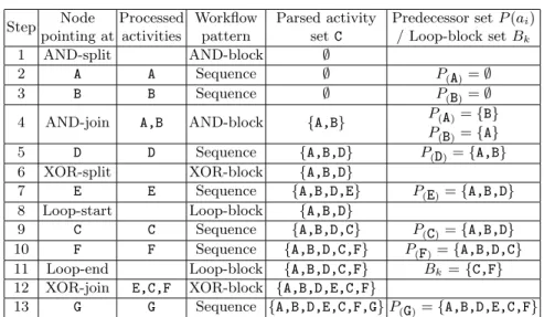
As example take process model S in Fig. 1. Table 1 shows analysis results after every step of function ParseModel from Algorithm 1. It indicates which node functionparseModel points to, which activities are processed, which pro- cess patterns it belongs to, to which set C changes afterwards, and what are the predecessor sets or loop-blocks obtained in this step. For example, Step 1 shows initial state of this function. Steps 2 and 3 analyze the two branches of the AND-block separately, and results are merged in Step 4. After processing activ- ity Din Step 5, the algorithm handles the XOR-block in Steps 6-12. Note the differences between Step 4 and Step 12 when dealing with XOR- and AND-joins respectively: additional changes are performed on predecessor sets for activi- ties corresponding to an AND-block. The Loop-block in S, in turn, is handled in Steps 8 - 11, during which we identify which activities are included in this Loop-block.
After obtaining predecessor setsP(ai) for every activityai∈N using func- tion parseModel, we can determine order relations between two activities as follows:
– If ((ai∈P(aj))∧ ¬(aj ∈P(ai))),Aaiaj = ’1’, i.e.,ai always precedesaj. – If (¬(ai∈P(aj))∧(aj ∈P(ai))),Aaiaj = ’0’, i.e.,ai always succeedsaj. – If ((ai ∈P(aj))∧ (aj ∈ P(ai))),Aaiaj = ’+’, i.e., ai appears before aj in
some traces while it succeedsaj in other traces.
Step Node Processed Workflow Parsed activity Predecessor setP(ai) pointing at activities pattern setC / Loop-block setBk
1 AND-split AND-block ∅
2 A A Sequence ∅ P(A)=∅
3 B B Sequence ∅ P(B)=∅
4 AND-join A,B AND-block {A,B} P(A)={B}
P(B)={A}
5 D D Sequence {A,B,D} P(D)={A,B}
6 XOR-split XOR-block {A,B,D}
7 E E Sequence {A,B,D,E} P(E)={A,B,D}
8 Loop-start Loop-block {A,B,D}
9 C C Sequence {A,B,D,C} P(C)={A,B,D}
10 F F Sequence {A,B,D,C,F} P(F)={A,B,D,C}
11 Loop-end Loop-block {A,B,D,C,F} Bk ={C,F}
12 XOR-join E,C,F XOR-block {A,B,D,E,C,F}
13 G G Sequence {A,B,D,E,C,F,G}P(G)={A,B,D,E,C,F}
Table 1.Analysis result for process modelS from Fig. 1 when applyingparseModel in Algorithm 1
– If (¬(ai∈P(aj))∧ ¬(aj ∈P(ai))),Aaiaj = ’-’, i.e.,ai andaj never appear together.
The abovementioned method is described by functioncomputeOrderRelationBasedOnPredecessorSets in lines 32 - 38 in Algorithm 1. The computation of these four order relations
{1,0,+,-} is straightforward since it directly matches with the definition of an order matrix (cf. Def. 3).
As discussed in Section 3, if a process model S contains Loop-blocks, its trace set TS becomes infinite. Therefore we need to reduce TS to simplified trace set TS0 for further analysis (cf. Def. 2). We can achieve this reduction by defining one silent activity τk for every Loop-block Bk to represent the it- erative behavior of the traces producible by Bk (cf. Section 3). After adding activity τk to the order matrix, the challenge is to determine order relations between τk and the other activities. In the following, we introduce function addSilentActivitiesForLoopStructure(Lines 39 - 48 in Algorithm 1) to de- termine order relations betweenτk and others. In principle, we can divide activ- ities into two groups:
– ai ∈Bk. Ifai is contained in the Loop-block, order relation betweenai and τk is straightforward. According to Definition 3,Aaiτk=0L0 andAτkai =0 L0 must hold.
– ai ∈N \Bk. In this case, we need to determine order relation between τk
and activityai which is outside the loop blockBk. Since our process model is block-structured, we can consider whole Loop-blockBk as single ”process step” in this context. Therefore, ”process step” should have unique order relations with the remaining activities. This implies that all activities be- longing to block Bk, including silent activity τk, should have same order
relation in respect to the activities located outside this block. We can there- fore determine relation betweenτk andai ∈N\Bk by considering another activityaj ∈Bk. Since both τk andaj belong to a same Loop-block,Aaiτk
can be assigned toA0aiaj. Similarly, we obtainAτkai=A0ajai.
For example take S from Fig. 1. Table 1 depicts predecessor set P(ai) of each activity ai, and the set Lfor Loop-blocks which we obtain when applying function parseModel in Table 1. Based on this, we can compute order ma- trix A using functions computeOrderRelationBasedOnPredecessorSets and addSilentActivitiesForLoopStructure. The result is shown in Fig. 1b. Spe- cial attention should be paid to the order relations between silent activityτ and the other activities: except the order relations betweenτ on the one hand andC andFon the other hand are ’L’, the order relations betweenτand the remaining activities are same as the ones CandFhave.
Complexity of Algorithm 1 is O(2n2) where n equals the number of activ- ities the process model has. To be more precise, the complexity of function parseModel isO(n2) and complexity of the other two functions corresponds to O(n2) in total. This polynomial complexity allows us to quickly transform a (large) process model into its order matrix for further analysis.
5 Transforming an Order Matrix back into a Process Model
In Section 4, we have introduced an algorithm for transforming a process model S into its corresponding order matrixA. In this section, we show how such an order matrixAcan be transformed back into a process modelS. This approach is described by Algorithm 2.
Algorithm 2 starts with defining a hashtable which maps activities from the order matrix (the key of the hashtable) to their corresponding blocks (the value of the hashtable). Initially, every activity from the order matrix constitutes a block itself (Line 2). The key idea of Algorithm 2 is to merge such blocks. More precisely, two blocks can form a bigger one iff they have same order relations in respect to all remaining blocks within the order matrix (Lines 6 - 9). If two blocks Bi andBj can be merged into a bigger block Bij, we can build the new block based on these two smaller blocks and their order relation (Lines 11 - 12).
The newly created block Bij replacesBi and Bj in the hashtable. We can then map such block to activityaiin the order matrix and remove the corresponding row and column for aj in A (Lines 13 - 15). Therefore, in every iteration, we reduce one row and one column of the order matrix. Merging blocks continues iteratively until there are only two blocks remaining in the order matrix. We merge these two blocks in the last step (Line 23).
FunctioncreateModel(BlockBi, BlockBj, OrderRelation3) creates a pro- cess model by merging two blocks Bi and Bj based on their order relation 3 (Lines 19 - 35 in Algorithm 2). If3represents a predecessor or successor relation, we just need to add one edge between start and end of these two blocks. If the
input : An order matrixA
output: A process modelS= (N, E, . . .) Define HashtableMap;
1
Define each activityaias a blockBi;Map.put(ai,Bi)i= (1, . . . , n);
2
iteration= 0; /* initial state */;
whileiteration< n−2do
3
foreachai, aj∈N, ai6=aj do
4
merge= True ;
5
forak∈N\ {ai, aj}do
6
if Aaiak6=Aajak then
7
merge= False;
8
/* two blocks can merge into a bigger one, iff they have same order relations to the others */;
break ;
9
if mergethen
10
createModel(Map.getValue(ai),Map.getValue(ai),Aaiaj)
11
/* create a new block based on the two blocks and their order relation */;
Bij =buildBlock(Map.getValue(ai),Map.getValue(ai),Aaiaj) ;
12
/* Merge these two block based on their order relation */; Map.remove(ai);Map.remove(aj) /* change the blocks */;
13
A.remove(aj) /* change order relations */;
14
Map.put (ai, Bij) ;
15
break;
16
iteration++;
17
S=createModel(Map.getValue(a1),Map.getValue(a2),Aa1a2) /* Merge last
18
two blocks */;
createModel(BlockBi, BlockBj, OrderRelation3) begin
19
if 3= ’0’ then
20
/* Merge block Bi and Bj based on their order relation 3 */
addEdge (Bj.end,Bi.start);
else if 3= ’1’ then
21
addEdge (Bi.end,Bj.start);
22
else if 3= ’+’ then
23
addNode (AND-split); addNode(AND-join) ;
24
addEdge (AND-split,Bi.start); addEdge (AND-split,Bi.start);
25
addEdge (Bj.end, AND-join); addEdge (Bj.end, AND-join) ;
26
else if 3= ’-’ then
27
addNode (XOR-split); addNode(XOR-join);
28
addEdge (XOR-split,Bi.start); addEdge (XOR-split,Bi.start);
29
addEdge (Bj.end, XOR-join); addEdge (Bj.end, XOR-join) ;
30
else if 3= ’l’ then
31
LetBi=τ; addNode (loop-start); addNode(loop-end) ;
32
addEdge (loop-start,Bj.start); addEdge (Bj.end,loop-end);
33
addEdge (loop.end, loop-start, loop) ;
34
end
35
Algorithm 2: Transforming an order matrix into a process model
two blocks have order relation ’+’ or ’-’, we add them to different branches of an AND- or XOR-block. If order relation3corresponds to ’L’, there must be a Loop-block in the process model and eitherBiorBj correspond a silent activity τ. Reason is that any silent activity τ can only be clustered with Loop-block B that it corresponds to. If Bi equals τ, we only need to surround Bj with a loop-backward edge.
As example take order matrixA from Fig. 1. Since activities Aand Bhave same order relations in respect to the remaining activities, we are able to merge these two activities to an AND-block. After creating this block, we remove ac- tivityBfrom order matrixA. For example, the block containingAandBcan be merged with activityDin order to create a bigger block. If we repeat this process of merging blocks, we finally obtain process modelS as depicted in Fig. 1.
6 One-to-one Mapping between a Process model and its Order Matrix
Section 4 has introduced Algorithm 1 for transforming a process model into its order matrix. In Section 5, we have further provided Algorithm 2 for transforming an order matrix back into its corresponding process model. Generally, it is critical to prove that such transformation constitutes a one-to-one mapping, i.e., if we first transform a process model S into its order matrix A, and then transform Aback to a process modelS0,S0 should be same asS.
When transforming a process model into an order matrix (cf. Algorithm 1), we recursively analyze each block of the process model from start to end.
However, when transforming an order matrix back into a process model (cf.
Algorithm 2), the order in which we merge blocks is more or less arbitrary, i.e., we merge two blocks together whenever this is possible. Therefore, it is important to know whether the order relation satisfies theassociative law, i.e., whether the order to merge small blocks into bigger ones can influence the result.
Let us first consider predecessor-successor order relations ’0’ and ’1’. Assume process model S contains three blocks Bi, Bj and Bk with Bi preceding Bj
and Bj preceding Bk. Obviously, we obtain ABiBj =0 10 and ABjBk =0 10. Representing this as mathematical equation, we obtainBi3Bj3Bkwith3being
’1’. If we need to transform order matrixAinto a process modelS0, it does not matter whether we first merge Bi and Bj or we first merge Bj and Bk, i.e., (Bi3Bj)3Bk=Bi3(Bj3Bk). It is obvious from Algorithm 2 that we only need to add control edges between the end of the preceding block and the start of the succeeding one. Therefore the order of adding edges does not influence the resulting model. Clearly, such rule also applies if order relation 3 corresponds to ’0’.
For order relations ’+’ and ’-’, let us re-assume that there are three blocksBi, Bj andBk with same order relation ’-’ among each other, i.e.,Bi3Bj3Bk with 3being ’-’. Fig. 2a shows two modelsS andS0 that result when merging these three blocks together. To be more precise,Scan be obtained by first mergingBi
andBj and then merging the intermediate block withBk (S = (Bi3Bj)3Bk),
while S0 can be obtained by first merging Bj and Bk and then merging the resulting block withBi(S0 =Bi3(Bj3Bk)).
a)b)
AND-Split AND-Join XOR-Split XOR-Join
S S’
S S’
S, S’ and S’’ are trace equivalent Bk
Bj
Bi
Bk
Bj
Bi
Bj
Bi
Bk
Bj
Bi
Bk
S’’
S’’
Bi
Bj
Bk
Bi
Bj
Bk
Fig. 2.Trace equivalence for AND and XOR blocks
Obviously, process models S and S0 are structurally different. However, S and S0 are trace equivalent despite their structural difference, i.e., trace sets TS and TS0 producible on S and S0 respectively are the same: TS = TS0 = TBi
STBj
STBk. Note that the two process models are trace equivalent toS00 as well. RegardingS00,Bi,Bj andBk are located in three different branches of the same XOR-block. In the context of our research, we consider S,S0 andS00 being the same, since the corresponding process models have same trace set and therefore show same behaviors.8This indicates that order relation ’-’ satisfies the associative law, and consequently the order in which blocks are merged is not relevant. When first transforming a process model (e.g.,S00) into order matrixA, and then transformingAback into a process model (e.g.,S0), the original and the newly derived process models are trace equivalent. In our context, we consider these two models being same. Thus the transformation between process model and order matrix constitutes a one-to-one mapping. Obviously, same results are obtained if the order relations between them are ’+’ (cf. Fig. 2b).
For order relation ’L’, the associative law is not applicable in the given context becauseBi3Bj3Bk (with3= ’L’) is not possible for an order matrix. IfBi3Bj
holds with3= ’L’, eitherBi or Bj must beτ. This, in turn, indicates that in expression Si3Sj3Sk, two out of the three blocks constitute silent activities τ. Let us assume that Bj and Bk are these two silent activities. Thus such expression means that blockBi is surrounded by a loop-backward edge to form a loop-block Bi0 and this Loop-block Bi0 is immediately surrounded by another loop-backward edge to form another Loop-block Bi00, i.e., Bi is surrounded by two loop-backward edges. In this case, Bi0 and Bi00 are trace equivalent, and
8 Like most process mining techniques (e.g. [30, 7, 34]), the stronger notion of bi- similarity are not considered in our context [9]
therefore expressionSi3Sj3Sk would be simplified toSi3Sj with3being ’L’.9 This implies that the condition to analyze the associative law does not hold.
Although associative law is not applicable to order relation ’L’, it cannot influence the one-to-one mapping between a process model and its order matrix.
Reason is that whenever two blocks have order relation ’L’, one of them must be a silent activity τ, and this silent activity can only be merged with the block surrounded by a loop-back edge. Assume that blockB is surrounded by a loop, i.e., has order relation ’L’ with silent activityτ (cf. Def. 3). For any block Bi which is different from B, there are only two situations: either B contains activities not inBiorBiis a sub-block ofB. In the first scenario, for any activity ai∈/B,ai must have different order relation in respect toτ than activities inB have, thereforeBicannot be clustered withτ; in the second scenario, there must be an activityai∈B\Bihaving different order relation toτ when compared to an activityaj∈Bi. ThereforeBican not be clustered withτ. This indicates that the silent activityτcan only be clustered with the Loop-block it corresponds to.
Consequently, the order of clustering also does not influence results.
7 Algebraic Properties of Order Relations
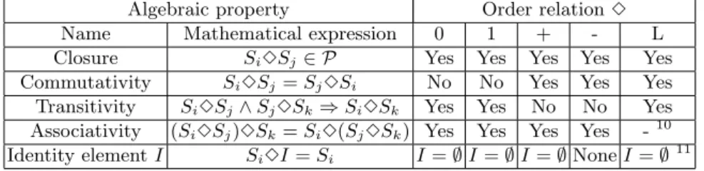
In addition to associativity of order relations, we have analyzed their algebraic properties. Let Si, Sj, Sk ∈ P be three sound process models. In this context, we denote a process model as sound if there are no deadlocks or unreachable activities in the process model [21, 28]. Let further 3 ={0,1,+,−, L} be the order relations as set out by Definition 3. Then, the algebraic system<P,3>
has the properties depicted in Table 2:
Algebraic property Order relation3
Name Mathematical expression 0 1 + - L
Closure Si3Sj∈ P Yes Yes Yes Yes Yes
Commutativity Si3Sj=Sj3Si No No Yes Yes Yes Transitivity Si3Sj∧Sj3Sk⇒Si3Sk Yes Yes No No Yes Associativity (Si3Sj)3Sk=Si3(Sj3Sk) Yes Yes Yes Yes -10 Identity elementI Si3I=Si I=∅I=∅I=∅NoneI=∅11
Table 2.The algebraic properties of order relation
9 We can easily identify such situation from the process model or the order matrix. If a block is surrounded by two loop-back edges in a process model, we only need to keep one of them so that the model is still trace equivalent to the original one. In an order matrix, we can easily identify such situation by checking whether two silent activitiesτ is able to merge or not. If yes, then we can remove one of them.
9 According to the analysis in Section 6, conditions for analyzing associative law does not exist
11If two blocksSi andSj have order relation ’L’, at least one of them must be silent activityτ. Therefore, we consider the identity element also being existent for order