Article
A Spaceborne Multisensory, Multitemporal Approach to Monitor Water Level and Storage Variations of Lakes
Alireza Taravat1,*, Masih Rajaei2, Iraj Emadodin3, Hamidreza Hasheminejad2, Rahman Mousavian4and Ehsan Biniyaz5
1 GEOMAR Helmholtz Centre for Ocean Research, 24105 Kiel, Germany
2 The Geoinformatics Experts Group, 8514143131 Najafabad, Iran; mrajaei@geoinformatics.co (M.R.);
hasheminejad@geoinformatics.co (H.H.)
3 Institute for Ecosystem Research, Christian Albrechts University, 24118 Kiel, Germany;
iemadodin@ecology.uni-kiel.de
4 Faculty of Engineering, Putra University, 43400 Serdang, Malaysia; mousavian.rahman@gmail.com
5 Geoinformation Center, Christian Albrechts University, 24118 Kiel, Germany; ebiniyaz@gis.uni-kiel.de
* Correspondence: art23130@gmail.com; Tel.: +49-431-600-4487 Academic Editor: Frédéric Frappart
Received: 15 July 2016; Accepted: 17 October 2016; Published: 25 October 2016
Abstract:Lake Urmia, the second largest saline Lake on earth and a highly endangered ecosystem, is on the brink of a serious environmental disaster similar to the catastrophic death of the Aral Sea.
Progressive drying has been observed during the last decade, causing dramatic changes to Lake Urmia’s surface and its regional water supplies. The present study aims to improve monitoring of spatiotemporal changes of Lake Urmia in the period 1975–2015 using the multi-temporal satellite altimetry and Landsat (5-TM, 7-ETM+ and 8-OLI) images. In order to demonstrate the impacts of climate change and human pressure on the variations in surface extent and water level, Lake Sevan and Van Lake with different characteristics were studied along with the Urmia Lake. Normalized Difference Water Index-Principal Components Index (NDWI-PCs), Normalized Difference Water Index (NDWI), Modified NDWI (MNDWI), Normalized Difference Moisture Index (NDMI), Water Ratio Index (WRI), Normalized Difference Vegetation Index (NDVI), Automated Water Extraction Index (AWEI), and MultiLayer Perceptron Neural Networks (MLP NNs) classifier were investigated for the extraction of surface water from Landsat data. The presented results revealed that MLP NNs has a better performance in the cases where the other models generate poor accuracy. The results show that the area of Lake Sevan and Van Lake have increased while the area of Lake Urmia has decreased by ~65.23% in the past decades, far more than previously reported (~25% to 50%). Urmia Lake’s shoreline has been receding severely between 2010 and 2015 with no sign of recovery, which has been partly blamed on prolonged droughts, aggressive regional water resources development plans, intensive agricultural activities, and anthropogenic changes to the system. The results also indicated that (among the proposed factors) changes in inflows due to overuse of surface water resources and constructing dams (mostly during 1995–2005) are the main reasons for Urmia Lake’s shoreline receding. The model presented in this manuscript can be used by managers as a decision support system to find the effects of building new dams or other infrastructures.
Keywords: water management; drought monitoring; long-term change detection; anthropogenic activities; wetland identification
1. Introduction
Lakes and rivers are the most accessible inland water resources available for ecosystems and human consumption [1] and they are valued for their ability to store floodwaters, protect shorelines,
Water2016,8, 478; doi:10.3390/w8110478 www.mdpi.com/journal/water
Water2016,8, 478 2 of 19
improve water quality, and recharge groundwater aquifers [2,3]. Therefore, the information of the long-time lake water storage variations is fundamental for understanding the impact of climate change and human activities on the water resources [4]. For these reasons, many responsible organizations operate a number of inland water level stations to collect information for water resources management [1,5–7]. However, still many remotely located lakes have not been gaged, especially in developing countries [8–10].
Because of the use of advance techniques (e.g., remote sensing), the number of gaging stations have decreased in recent years around the globe [5,6,8,11]. Remote sensing technology for monitoring changes is widely used in different applications such as land use/cover change [12,13], disaster monitoring [14,15], forest and vegetation changes [16,17], urban sprawl [18,19], and hydrology [20,21].
The knowledge about water resources can be efficiently improved by the use of remote sensing which include radar, microwave, infrared, and visible sensors. Among the mentioned remote sensing methods, microwave remote sensing provides a unique capability for mapping inundation area and delineate water boundaries over large areas of the Earth’s land surface [5,22]. The exploitation of satellite data about water bodies provide reliable information for the assessment of present and future water resources, climate models, agriculture suitability, river dynamics, wetland inventory, watershed analysis, surface water survey and management, flood mapping, and environment monitoring, which are critical for sustainable management of water resources on the Earth [1,23–25].
Lake surface areas (especially closed lakes) [1] are sensitive to natural changes and thus may serve as significant proxies for variations in regional environmental and fluctuations in global climate [26–28].
Changes in the areal extent of lake surface water may occur due to various factors, including the progressive unveiling of the lake basin by sediments, climate change, tectonic activity causing uplift or subsidence, and the development of drainage faults [27,29,30].
Satellite remote sensing for the analysis of water volume variation has been used very often in the related literature [31]. Birkett [32], Frappart et al. [33] and Crétaux et al. [11] have used successfully satellite radar altimetry to derive water levels of water bodies [8]. Duan et al. [8] estimated water volume variations in Lake Mead from four satellite altimetry and imagery datasets [31]. Recently, Baup et al. [34] combined high-resolution satellite images and altimetry to estimate the volume changes of the lakes that are mainly used for irrigation in France [31]. Surface water volume changes derived from the combination of altimetry and imagery were removed from the total water storage anomaly estimated using observations from the GRACE gravimetry from space mission to estimate soil water content variations [35–37].
Yan et al. [38] detected the dynamic changes in surface areas of Lake Qinghai using Landsat TM/ETM+ images based on the model which relies on the fact that water bodies appear dark in middle and near infrared bands [1,39]. These studies provide reliable estimation of lake fluctuation in water levels and areas, which is of great significance for water resources management under the background of climate change [1]. However, these studies have focused on the detection and analysis of variations in surface extent and water level in response to either climate change or human-environment interactions [1,40].
Among the models proposed for water feature extraction from satellite data, multi-band ratio models are the most popular models for surface water extraction [27]. Komeili et al. [41] developed NDWI-PCs model based on Normalized Difference Water Index (NDWI) and Principal Component Analysis (PCA) for extracting water features from Landsat TM, ETM+, and OLI imagery over Lake Urmia. Xu [42] developed a modified NDWI (MNDWI) in which the middle infrared (MIR) band was replaced with the near infrared (NIR) band in order to decrease false positive from built-up lands.
Ouma et al. [43] developed a Water Index (WI) model using Tasseled Cap Wetness (TCW) index and NDWI for Landsat TM and ETM+ imagery over Rift Valley lakes in Kenya [27].
The other proposed models include semi-automated change detection approaches [27], e.g., single band density slicing and Maximum Likelihood (MXL) model presented by Frazier et al. [44], conceptual clustering technique and dynamic thresholding proposed by Soh et al. [45], supervised
classification model proposed by Alecu et al. [46], multivariate regression method [47] and automated spectral-shape procedure presented by Yang et al. [48]. The last but not least proposed algorithms are automatic extraction methods, for instance, Support Vector Machine (SVM) and Spectral Angle Mapper (SAM) models presented by Jawak et al. [49], object oriented multi-resolution segmentation model developed by Shao et al. [50], and fuzzy intra-cluster distance within the Bayesian algorithm proposed by Jeon et al. [51]. To the best of the authors’ knowledge, a detailed analysis of Artificial Neural Networks (ANNs) models for automatic surface water extraction has not yet been presented in the related literature, whereas ANNs models can be very competitive in terms of accuracy and speed for image classification.
Starting from these motivations, the purpose of the present paper is to demonstrate: (1) the potential of ANNs approach for a fast, robust, accurate and automated water feature extraction without using any ancillary data; and (2) the detection and analysis of variations in surface extent and water level in response to both climate change and human-environment interactions using multisensory remote sensing techniques.
In order to examine the robustness of the algorithm, the result of the proposed model has been compared with the results of different satellite-derived indexes including Normalized Difference Water Index (NDWI) [41,52], Modified Normalized Difference Water Index (MNDWI) [42], Water Ratio Index (WRI) [41,53], Normalized Difference Vegetation Index (NDVI) [41,54], Automated Water Extraction Index (AWEI) [41,55], and Normalized Difference Water Index (NDWI) and Principal Component Analysis (NDWI-PCs) [41] models, which are the latest models published in the related literature about extraction of surface water from satellite imagery. The datasets (for the period 1975–2015) prepared over Urmia Lake, Lake Sevan, and Van Lake (situated in similar geographical regions) have been used in the Experimental Section because the mentioned lakes are under intensive natural and human driving forces.
The paper starts with a description of our study areas in Section 2. Section 3 describes complementary datasets that have been used in this paper. In Section4, our approach and algorithms to extract and analyse the surface water extent of the lakes using satellite imagery has been shown.
The proposed model, which has been used for deriving the lakes water levels and lakes surface areas from satellite data, is presented in Section5. The results from satellite altimetry and satellite imagery, together with local climate data, are used in the same section for discussing about the impact of factors such as climate change and anthropogenic activities on the drying up of the studied lakes. Section6 will summarize and conclude the results of this study.
2. Study Areas
2.1. Urmia Lake
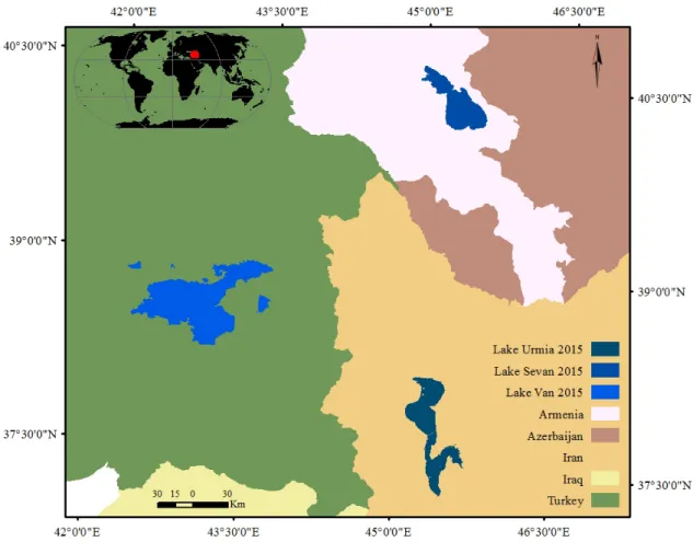
The Urmia Lake basin is located in the northwest of Iran at ~37◦N and 45◦E (Figure1). In Urmia Lake basin, the elevation increases from 1174 m at Urmia Lake to 3861 m above sea level in the Sahand Mountains [56]. The main water of the lake is supplied from 21 seasonal or permanent (the main inputs are Zarrine-Rud, Aji Chay, Baran duz, and Godard), and 39 periodic rivers and springs [57,58].
The watershed area covered about 52,000 km2 which is 3% of Iran’s land [59]. The basin with 6.4 million inhabitants is important in terms of housing, industrial and agricultural activities for the East Azerbaijan Province in Iran [56,60].
A unique feature of Lake Urmia is its hypersaline environment, with salinity ranging from 217 to more than 300 g/L, approximately eight times higher than seawater [57,61–63]. Lake Urmia, with its 102 islands, is defined as a national park and international biosphere reserve by UNESCO (United Nation Education, Scientific and Cultural Organization) because of its ecological importance [64–67].
Climate in the lake’s basin is controlled by the mountains surrounding the lake. Urmia Lake is situated in a semi-arid area, having a temperature range between ~0◦C and−20◦C in winter and up to ~40◦C in summer with a mean annual temperature of 11.2◦C, an average precipitation and
Water2016,8, 478 4 of 19
evaporation rate of 341 and 1200 mm/year, respectively. The annual average evaporation from the lake surface is ~1 m [58,67–69]. The intensity of bird migration (there are 212 species) to the area highly depends on the primary production of Lake Urmia, and particularly on availability of salt-adjusted brine shrimp [57,70,71].
There are 9 cities adjacent to the lake, where agriculture is the main part of the economy and the major source of income for the communities. About 70% of cultivated lands in western part of the lake are wheat lands. The other main crops are oats, fruits, and vegetables (especially grape and apple).
During 1979 to 2006, irrigated land in the watershed area increased by 8% of the Urmia’s watershed area [72]. Construction of the 15 km highway in the early 1990s across the lake has divided the lake into two parts (35.5% in north and 64.5% in south) [72].
2.2. Lake Sevan
Lake Sevan is situated in the northern part of the Armenian Volcanic Highland at ~45.2◦E and 40◦N (Figure1), in Gegharkhounik Marz Province. In Lake Sevan basin the elevation increases from 1854 m at Sevan Lake to 3583 m above sea level in the Sevana, Vardenis and Geghama Mountains.
A peculiarity of Lake Sevan includes the small ratio between the catchment and surface area of the lake is only 3:1, compared to other major lakes (10:1 on average) [73]. Lake Sevan has comparatively
“soft water” (mineralization = 700 mg/L) [73] in comparison with the other neighbouring great lakes like Lake Van, Caspian Sea, and Urmia Lake.
Twenty-eight rivers and streams flow into Lake Sevan, and the River Hrazdan flows out of the lake. The average annual temperature of the lake is 5◦C. Annual precipitation ranges from 340 to 720 mm, of which 17% falls in the winter, 37% in the spring, 26% in the summer and 20% in the autumn [74]. There are six species of fishes in the Lake Sevan basin. The lake is an important stop for migratory birds (210 species), especially in October–December before the lake becomes covered with ice [75]. The main economic activities in the basin are agriculture and fisheries. Approximately 20% of the livestock in the country is raised in the basin. Ninety per cent of fish catch and 80% of crayfish catch of Armenia is from Lake Sevan [76].
The outflow of water from the lake has been artificially regulated since 1933 during the Soviet period for hydropower and irrigation. Before the increased artificial outflow, the surface of Lake Sevan was at an altitude of 1916.20 m with a surface area of 1416 km2and volume of 58.5 km3. The water-level decreases from this artificial outflow process influenced an array of hydrological and ecological conditions at the lakeshore and in the lake [77].
2.3. Van Lake
Van Lake (with the large drainage basin of 12,500 km2) is a saline closed-basin lake located (~43◦E and 38.30◦N) in Eastern Anatolia, Turkey (Figure1). It is the largest lake in Turkey and the largest soda lake in the world [78]. The average elevation of basin is 2829 m above mean sea level that increases from ~1626 m at the lake to 4032 m above sea level in mountain regions. The total surface area of its catchment basin is about 5000 km2[79].
Several rivers and streams (including the Karasu, Hosap, Güzelsu, Bendimahi, Zilan and Yeniköprü Streams) flow into Van Lake without any outlet. The lack of outflows causes the accumulation of salts in the lake and increases the salinity because of the water discharges by evaporation [78,80]. The local climate of the Lake Van area is characterized by strong seasonality, expressed as cold winters from December to February with mean temperatures below 0◦C, and warm, dry summers in July and August with mean temperatures exceeding 20◦C. Cold, dry air masses originating from high northern latitudes acquire moisture when passing over the Mediterranean Sea, reaching Lake Van from the southwest [81,82]. Annual precipitation ranges from 400 to 700 mm [83].
According to Aksoy et al. [78], because of the high water salinity of the lake, it cannot be used for drinking or irrigation and also only limited species of fresh water fish could survive in this condition.
The natural vegetation is steppe dominated by sub-euxinian oak forest; however, there is hardly any
natural vegetation left, and instead, there is a predominance of agricultural land [68,84]. In the last decade, the water level in Van Lake has risen ~2 m and, consequently, the low-lying inundated along the shore are now concerning local administrators and government official, and affecting irrigation activities and people’s properties [85].
hardly any natural vegetation left, and instead, there is a predominance of agricultural land [68,84].
In the last decade, the water level in Van Lake has risen ~2 m and, consequently, the low‐lying inundated along the shore are now concerning local administrators and government official, and affecting irrigation activities and people’s properties [85].
Figure 1. The geographical locations of Lake Urmia, Lake Sevan, and Van Lake in Middle East.
3. Data
3.1. Landsat and Digital Elevation Model (DEM) Dataset
The model, which has been used in the classification phase, is trained and tested on Landsat database. The training and test datasets consist of the mosaicked Landsat images for each five years (from the same season) from 1975 to 2015. Each study area contains nine mosaicked Landsat images (total 81 images for all three study areas). All of the images have been obtained from the US Geological Survey (USGS) Global Visualization Viewer [82].
Digital Elevation Model (DEM) maps have been extracted from Shuttle Radar Topography Mission (SRTM) 1‐Arc‐Second global data. SRTM 1‐Arc‐Second global elevation data offer worldwide coverage of void filled data at a resolution of 30 meters (1‐arc‐second) and provide open distribution of this high‐resolution global dataset [83].
3.2. Radar Altimetry Dataset
Altimetry, as the only source of information for most lakes in remote areas, is a technique that has a proven potential for hydrology science [69]. GEOSAT (1986–1988), ERS‐1 (1991–1996), Topex/Poseidon (1992–2005), GFO (2000–2008), ERS‐2 (1995–2011), ENVISAT (2002–2012), Jason‐1 (2001–), Jason‐2 (2008–), Altika (2013–), Sentinel‐3 (2016–), and Jason‐3 (2016–) are several satellite altimetry missions that have been launched since the late 1980s. The combined global altimetry datasets have more than two‐decade‐long history and are being continuously updated [86,87].
Figure 1.The geographical locations of Lake Urmia, Lake Sevan, and Van Lake in Middle East.
3. Data
3.1. Landsat and Digital Elevation Model (DEM) Dataset
The model, which has been used in the classification phase, is trained and tested on Landsat database. The training and test datasets consist of the mosaicked Landsat images for each five years (from the same season) from 1975 to 2015. Each study area contains nine mosaicked Landsat images (total 81 images for all three study areas). All of the images have been obtained from the US Geological Survey (USGS) Global Visualization Viewer [82].
Digital Elevation Model (DEM) maps have been extracted from Shuttle Radar Topography Mission (SRTM) 1-Arc-Second global data. SRTM 1-Arc-Second global elevation data offer worldwide coverage of void filled data at a resolution of 30 meters (1-arc-second) and provide open distribution of this high-resolution global dataset [83].
3.2. Radar Altimetry Dataset
Altimetry, as the only source of information for most lakes in remote areas, is a technique that has a proven potential for hydrology science [69]. GEOSAT (1986–1988), ERS-1 (1991–1996), Topex/Poseidon (1992–2005), GFO (2000–2008), ERS-2 (1995–2011), ENVISAT (2002–2012), Jason-1 (2001–), Jason-2 (2008–), Altika (2013–), Sentinel-3 (2016–), and Jason-3 (2016–) are several satellite altimetry missions
Water2016,8, 478 6 of 19
that have been launched since the late 1980s. The combined global altimetry datasets have more than two-decade-long history and are being continuously updated [86,87].
Over the past 10 years, HYDROWEB has developed a web database [4,69,88] containing time series over water levels of large lakes and wetlands on a global scale. The lake levels provided by HYDROWEB are based on the merged Topex/Poseidon, Jason-1 and 2, ENVISAT and GFO data.
The monthly level variations of almost 150 lakes and reservoirs are freely provided by multi satellite altimetry measurements.
4. Methods and Algorithms
4.1. An Overview of MultiLayer Perceptron Neural Networks (MLP NNs)
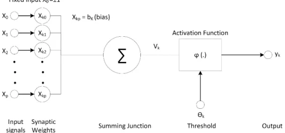
For applying a binary classification to extract water features, an artificial neural networks classifier has been used. Artificial Neural Networks (ANNs) algorithms classify regions of interest using a methodology that performs similar functions to the human brain such as understanding, learning, solving problems and taking decisions [89]. ANNs architecture consists of three units that include input layer, hidden layer and output layer (Figure2). In most ANNs models, hidden layers use non-linear activation functions for processing the data [90].
Water 2016, 8, 478 6 of 19
Over the past 10 years, HYDROWEB has developed a web database [4,69,88] containing time series over water levels of large lakes and wetlands on a global scale. The lake levels provided by HYDROWEB are based on the merged Topex/Poseidon, Jason‐1 and 2, ENVISAT and GFO data. The monthly level variations of almost 150 lakes and reservoirs are freely provided by multi satellite altimetry measurements.
4. Methods and Algorithms
4.1. An Overview of MultiLayer Perceptron Neural Networks (MLP NNs)
For applying a binary classification to extract water features, an artificial neural networks classifier has been used. Artificial Neural Networks (ANNs) algorithms classify regions of interest using a methodology that performs similar functions to the human brain such as understanding, learning, solving problems and taking decisions [89]. ANNs architecture consists of three units that include input layer, hidden layer and output layer (Figure 2). In most ANNs models, hidden layers use non‐linear activation functions for processing the data [90].
Figure 2. The block diagram shows the model of a neuron, which forms the basis for designing ANNs.
Formally, a one‐hidden‐layer MLP is a function ∶ → , where D is the size of input vector x and L is the size of the output vector , such that in matrix notation:
(1)
with bias vectors and ; weight matrices and ; and activation functions G and s.
The vector constitutes the hidden layer. Typical choices for s include tanh / or the logistic sigmoid function, with sigmoid 1/ 1 . The logistic sigmoid function ranges from 0 to +1. However, it is sometimes desirable to have the activation function range from −1 to +1, in which case the activation function assumes an anti‐symmetric form (e.g., tanh function) with respect to the origin [89,91].
4.2. Methodology
The considered dataset contains an overall number of 81 Landsat images (before mosaicking).
The methodology of this investigation is summarized and represented in Figure 3.
Figure 2.The block diagram shows the model of a neuron, which forms the basis for designing ANNs.
Formally, a one-hidden-layer MLP is a function f : RD → RL, whereDis the size of input vector xandLis the size of the output vector f(x), such that in matrix notation:
f(x) =G
b(2)+W(2)
s(b(1)+W(1)x) (1)
with bias vectors b(1) andb(2); weight matricesW(1)andW(2); and activation functions Gands.
The vectorh(x) =Φ(x) =s
b(1)+W(1)x
constitutes the hidden layer. Typical choices forsinclude tanh(a) = (ea−e−a)/(ea+e−a)or the logistic sigmoid function, with sigmoid(a) =1/ 1+e−1 . The logistic sigmoid function ranges from 0 to +1. However, it is sometimes desirable to have the activation function range from −1 to +1, in which case the activation function assumes an anti-symmetric form (e.g., tanh function) with respect to the origin [89,91].
4.2. Methodology
The considered dataset contains an overall number of 81 Landsat images (before mosaicking).
The methodology of this investigation is summarized and represented in Figure3.
Figure 3. Schematic representation of the methodology.
4.2.1. Image Pre‐Processing
As a pre‐processing task for image classification, radiometric calibration, atmospheric correction, mosaicking, and co‐registration have been applied to the datasets. Radiometric calibration and atmospheric correction were conducted according to Schroeder et al. [92]. All the images covering the study areas for each year were mosaicked and then co‐registered with less than 0.5 pixel of Root Mean Square Error (RMSE). Around 47 control points were selected for co‐registration of each image with the reference image.
The stripes in Landsat ETM+ data (caused by the SLC in the ETM+ instrument failed on 31 May 2003) have been removed according to Taravat et al. [93]. Pixels not affected by striping are used to construct spline functions describing spatial grey level distributions of an image [93].
The sub‐images containing the lakes basin for each lake were extracted using the Area of Interest tool of ENVI (Environment for Visualizing Images) software to make classification and image interpretation more expedient and focused (Figure 4). The data were then projected in geographical latitude/longitude projection and WGS84 datum. Furthermore, the image was exported into .TIFF format for further analysis.
4.2.2. Image Classification
After the pre‐processing phase, all images have been classified by MLP neural networks, which have been found to be the best suited topology for pixel level classifications [89]. In a multilayer perceptron model instead of feeding the input to the logistic regression, the hidden that has a nonlinear activation function layer(s) is used while the top layer is a soft max layer. The soft max function is the gradient‐log‐normalizer of the categorical probability distribution, which is used in various probabilistic multiclass classification methods including multinomial logistic regression, multiclass linear discriminant analysis, naive Bayes classifiers and artificial neural networks [94].
In MLP model, the connections between perceptrons are forward and every perceptron is connected to all the perceptrons in the next layer except the output layer that directly gives the result. MLP utilizes back propagation for training the network [90,91]. In the proposed model, Landsat data in spectral bands 480, 560, 660, and 825 nm have been used as the input of the model.
4.2.3. Models Comparison
In order to evaluate the performance of the proposed model for surface water extraction, the results have been compared with the results of MNDWI, AWEI, NDVI, NDWI, WRI, and NDWI‐PCs, which are the popular classifier methods presented in the latest papers published in the related literature about extraction of surface water from satellite imagery [41].
Figure 3.Schematic representation of the methodology.
4.2.1. Image Pre-Processing
As a pre-processing task for image classification, radiometric calibration, atmospheric correction, mosaicking, and co-registration have been applied to the datasets. Radiometric calibration and atmospheric correction were conducted according to Schroeder et al. [92]. All the images covering the study areas for each year were mosaicked and then co-registered with less than 0.5 pixel of Root Mean Square Error (RMSE). Around 47 control points were selected for co-registration of each image with the reference image.
The stripes in Landsat ETM+ data (caused by the SLC in the ETM+ instrument failed on 31 May 2003) have been removed according to Taravat et al. [93]. Pixels not affected by striping are used to construct spline functions describing spatial grey level distributions of an image [93].
The sub-images containing the lakes basin for each lake were extracted using the Area of Interest tool of ENVI (Environment for Visualizing Images) software to make classification and image interpretation more expedient and focused (Figure4). The data were then projected in geographical latitude/longitude projection and WGS84 datum. Furthermore, the image was exported into TIFF format for further analysis.
4.2.2. Image Classification
After the pre-processing phase, all images have been classified by MLP neural networks, which have been found to be the best suited topology for pixel level classifications [89]. In a multilayer perceptron model instead of feeding the input to the logistic regression, the hidden that has a nonlinear activation function layer(s) is used while the top layer is a soft max layer. The soft max function is the gradient-log-normalizer of the categorical probability distribution, which is used in various probabilistic multiclass classification methods including multinomial logistic regression, multiclass linear discriminant analysis, naive Bayes classifiers and artificial neural networks [94].
In MLP model, the connections between perceptrons are forward and every perceptron is connected to all the perceptrons in the next layer except the output layer that directly gives the result. MLP utilizes back propagation for training the network [90,91]. In the proposed model, Landsat data in spectral bands 480, 560, 660, and 825 nm have been used as the input of the model.
4.2.3. Models Comparison
In order to evaluate the performance of the proposed model for surface water extraction, the results have been compared with the results of MNDWI, AWEI, NDVI, NDWI, WRI, and NDWI-PCs, which are the popular classifier methods presented in the latest papers published in the related literature about extraction of surface water from satellite imagery [41].
Water2016,8, 478 8 of 19
Water 2016, 8, 478 8 of 19
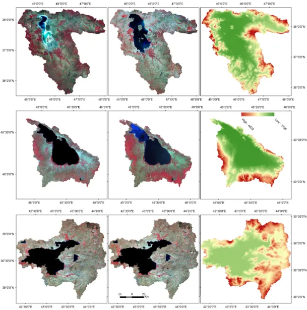
Figure 4. Standard false colour composite of Landsat imagery over Lake Urmia basin (first row);
Lake Sevan basin (second row); and Van Lake basin (third row) at two different epochs: 2015 (left column); and 1975 (middle column). In the right column of the figure, the elevation map of the basins has been shown.
4.2.4. Time Series Change Detection
In order to analyse the time series of height above reference surface variations of lakes which have been extracted from radar altimetry data, Pruned Exact Linear Time (PELT) algorithm has been used. PELT model is considered for identifying the points within a dataset where the statistical properties change. PELT model is based on the algorithm of Jackson et al. [95], but involves a pruning step within the dynamic program. Killick et al. [96] has proven that PELT model leads to a substantially more accurate segmentation than Binary Segmentation. In PELT model, a number of changes (m) together with their positions are:
τ
1: m = (τ
1, ,τ
m) (2) Each change position is an integer within (1, n − 1). “m” will split the data into m + 1 segments, with the ith segment containing y(τi−1 + 1):τi, where y is an ordered sequence of data. The general approach to identify multiple changes is defined as:Figure 4. Standard false colour composite of Landsat imagery over Lake Urmia basin (first row);
Lake Sevan basin (second row); and Van Lake basin (third row) at two different epochs: 2015 (left column); and 1975 (middle column). In the right column of the figure, the elevation map of the basins has been shown.
4.2.4. Time Series Change Detection
In order to analyse the time series of height above reference surface variations of lakes which have been extracted from radar altimetry data, Pruned Exact Linear Time (PELT) algorithm has been used.
PELT model is considered for identifying the points within a dataset where the statistical properties change. PELT model is based on the algorithm of Jackson et al. [95], but involves a pruning step within the dynamic program. Killick et al. [96] has proven that PELT model leads to a substantially more accurate segmentation than Binary Segmentation. In PELT model, a number of changes (m) together with their positions are:
τ1:m= (τ1, . . . ,τm) (2)
Each change position is an integer within (1,n−1). “m” will split the data into m + 1 segments, with theith segment containingy(τi−1+ 1):τi, whereyis an ordered sequence of data. The general approach to identify multiple changes is defined as:
m+1
∑
i=1
(C(y(τi−1+1):τi)) +βf(m) (3) whereCis a cost function for a segment andβf(m)is a penalty to guard against over fitting.
5. Results and Discussion
In order to detect the surface area changes of the lakes in the period 1975–2015, the water surface of each lake in each temporal image was extracted using MLP classifier. In the MLP classifier, 100,000 pixels (extracted from the Landsat dataset) have been used for training/testing the net.
The training sets contain 60% of the data, and the test sets contain the remaining 40%. Pixel selection for the training/test set has been performed randomly and repeated six times.
After the several attempts to properly select the number of units in the hidden layers, architecture 4-10-4 has been finally chosen for its good performance in terms of classification accuracy, Root-Mean Square Error (RMSE), and training time. In total, 35,000 training cycles were sufficient to train the network. The inputs of the net consist of Landsat data in spectral bands 480, 560, 660, and 825 nm, and the output provides the pixel classification in terms of water body, urban area, bare lands, and green lands. One MLP classifier has been used in classifying all the images (Figure5).
τ 1 : τ β (3)
where C is a cost function for a segment and β is a penalty to guard against over fitting.
5. Results and Discussion
In order to detect the surface area changes of the lakes in the period 1975–2015, the water surface of each lake in each temporal image was extracted using MLP classifier. In the MLP classifier, 100,000 pixels (extracted from the Landsat dataset) have been used for training/testing the net. The training sets contain 60% of the data, and the test sets contain the remaining 40%. Pixel selection for the training/test set has been performed randomly and repeated six times.
After the several attempts to properly select the number of units in the hidden layers, architecture 4‐10‐4 has been finally chosen for its good performance in terms of classification accuracy, Root‐Mean Square Error (RMSE), and training time. In total, 35,000 training cycles were sufficient to train the network. The inputs of the net consist of Landsat data in spectral bands 480, 560, 660, and 825 nm, and the output provides the pixel classification in terms of water body, urban area, bare lands, and green lands. One MLP classifier has been used in classifying all the images (Figure 5).
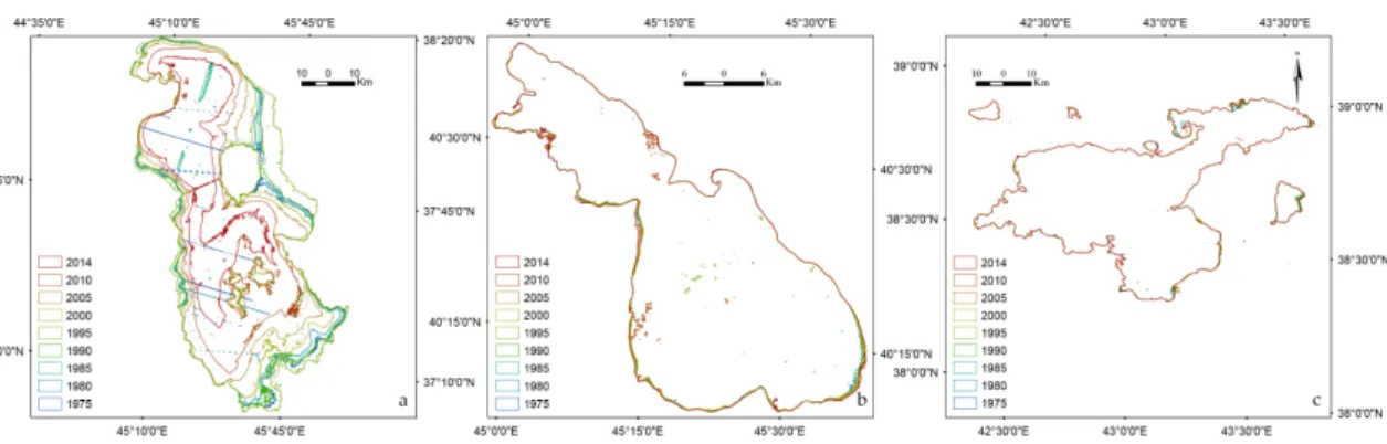
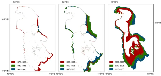
Figure 5. Temporal surface area changes (every five years) map in the period 1975–2015 for: (a) Urmia Lake; (b) Lake Sevan; and (c) Van Lake.
An accuracy assessment has been carried out in order to assess the classifiers more appropriately. For each of the 27 mosaicked images, 20,000 pixels (which is 6% of each image) have randomly been selected and then labelled by visual interpretation. The same procedure has been used to calculate the accuracy of the MNDWI, AWEI, NDVI, NDWI, WRI, and NDWI‐PCs classifiers for each of the 27 mosaicked images.
For visual interpretation, Landsat ETM+ data in spectral bands 560 nm, 660 nm, and 825 nm have been used in RGB format. The main reason for using this combination is the high contrast of water and dry/land areas (due to the high absorption and reflectance of NIR (825 nm) by water and the terrestrial vegetation and dry soil, respectively) in NIR band [31].
The accuracy of the whole dataset classified by MLP ANNs is 95.52% with a standard deviation of 2.00%, 3.88% and 4.47% commission (the samples which are committed to the wrong class) and omission (the samples which are omitted from the right class) errors and average, respectively. The average accuracy computed for the NDWI‐PCs (which generates the best results after MLP NNs) is 86.10% with a standard deviation of 2.47%, 7.67% and 13.90% commission and omission errors and average, respectively. An improvement of 9.42% in accuracy has been obtained on the dataset classified by MLP NNs with respect to the same dataset classified by the NDWI‐PCs model.
Moreover, MLP classifier generated less Commission error with respect to the NDWI‐PCs model.
The results of accuracy assessment applied to different models are displayed in Tables 1 and 2.
Figure 5. Temporal surface area changes (every five years) map in the period 1975–2015 for:
(a) Urmia Lake; (b) Lake Sevan; and (c) Van Lake.
An accuracy assessment has been carried out in order to assess the classifiers more appropriately.
For each of the 27 mosaicked images, 20,000 pixels (which is 6% of each image) have randomly been selected and then labelled by visual interpretation. The same procedure has been used to calculate the accuracy of the MNDWI, AWEI, NDVI, NDWI, WRI, and NDWI-PCs classifiers for each of the 27 mosaicked images.
For visual interpretation, Landsat ETM+ data in spectral bands 560 nm, 660 nm, and 825 nm have been used in RGB format. The main reason for using this combination is the high contrast of water and dry/land areas (due to the high absorption and reflectance of NIR (825 nm) by water and the terrestrial vegetation and dry soil, respectively) in NIR band [31].
The accuracy of the whole dataset classified by MLP ANNs is 95.52% with a standard deviation of 2.00%, 3.88% and 4.47% commission (the samples which are committed to the wrong class) and omission (the samples which are omitted from the right class) errors and average, respectively.
The average accuracy computed for the NDWI-PCs (which generates the best results after MLP NNs) is 86.10% with a standard deviation of 2.47%, 7.67% and 13.90% commission and omission errors and average, respectively. An improvement of 9.42% in accuracy has been obtained on the dataset classified by MLP NNs with respect to the same dataset classified by the NDWI-PCs model. Moreover, MLP classifier generated less Commission error with respect to the NDWI-PCs model. The results of accuracy assessment applied to different models are displayed in Tables1and2.
Water2016,8, 478 10 of 19
Table 1.The average values of commission and emission error (In %) achieved by different models for surface water extraction.
MinOm MaxOm MeanOm St.DevOm MinCm MaxCm MeanCm St.DevCm
MNDWI 13.60 26.80 23.69 3.75 17.60 25.50 15.02 3.09
AWEI 12.60 28.50 20.79 4.02 9.70 22.10 12.33 2.94
NDVI 10.80 30.00 20.28 5.26 9.30 30.39 14.95 6.16
NDWI 13.80 21.30 17.03 2.69 3.40 10.80 7.27 2.93
WRI 14.00 22.00 18.68 2.26 5.30 10.8 7.89 2.11
NDWI-PCs 10.80 18.00 13.90 2.47 4.50 10.80 7.67 2.36
MLP ANNs 2.50 10.00 4.47 2.00 1.40 8.50 3.88 2.19
Table 2.The average values of the accuracies for different types of anomalies.
Min % Max % Mean % St.Dev
MNDWI 73.20 86.40 76.33 3.73
AWEI 71.50 87.40 79.20 4.20
NDVI 70.00 89.20 79.71 5.27
NDWI 78.70 86.20 82.96 2.69
WRI 78.00 86.00 81.31 2.26
NDWI-PCs 82.00 89.20 86.10 2.47
MLP ANNs 90.00 97.50 95.52 2.00
The outputs of the MLP NNs classifier have been overlaid to produce the surface water changes (for each five year) in time-series started from 1975 to 2015 (Figure 6). The results show that the Urmia Lake surface area was ~4724.69 km2, ~4111.12 km2, ~3184.73 km2, and ~1642.71 km2in 2000, 2005, 2010, and 2015, respectively (Table3).
Water 2016, 8, 478 10 of 19
Table 1. The average values of commission and emission error (In %) achieved by different models for surface water extraction.
MinOm MaxOm MeanOm St.DevOm MinCm MaxCm MeanCm St.DevCm MNDWI 13.60 26.80 23.69 3.75 17.60 25.50 15.02 3.09
AWEI 12.60 28.50 20.79 4.02 9.70 22.10 12.33 2.94 NDVI 10.80 30.00 20.28 5.26 9.30 30.39 14.95 6.16 NDWI 13.80 21.30 17.03 2.69 3.40 10.80 7.27 2.93
WRI 14.00 22.00 18.68 2.26 5.30 10.8 7.89 2.11
NDWI‐PCs 10.80 18.00 13.90 2.47 4.50 10.80 7.67 2.36 MLP ANNs 2.50 10.00 4.47 2.00 1.40 8.50 3.88 2.19
Table 2. The average values of the accuracies for different types of anomalies.
Min % Max % Mean % St.Dev MNDWI 73.20 86.40 76.33 3.73
AWEI 71.50 87.40 79.20 4.20 NDVI 70.00 89.20 79.71 5.27 NDWI 78.70 86.20 82.96 2.69
WRI 78.00 86.00 81.31 2.26
NDWI‐PCs 82.00 89.20 86.10 2.47 MLP ANNs 90.00 97.50 95.52 2.00
The outputs of the MLP NNs classifier have been overlaid to produce the surface water changes (for each five year) in time‐series started from 1975 to 2015 (Figure 6). The results show that the Urmia Lake surface area was ~4724.69 km2, ~4111.12 km2, ~3184.73 km2, and ~1642.71 km2 in 2000, 2005, 2010, and 2015, respectively (Table 3).
Figure 6. Lake Urmia surface area change maps generated using MLP NNs classifier.
The Urmia Lake surface area has decreased ~613.57 km2 between 2000 and 2005, ~926.39 km2 between 2005 and 2010, and ~1542.02 km2 between 2010 and 2015, while the Lake Sevan and Van Lake surface areas have increased ~14.69 km2 and ~16.15 km2 between 2000 and 2005, 9.93 km2 and
~5.99 km2 between 2005 and 2010, and 3.57 km2 and ~1.37 km2 between 2010 and 2015, respectively.
The most intense changes in Urmia Lake is detected between 2010 and 2015, during which the lake lost ~65.23% of its surface area in comparison with the year 2000 and 48.41% of its surface area in comparison with the year 2010.
In order to analyse the time series of height above reference surface variations of lakes extracted from radar altimetry data, two models have been used. In the first model, the time series were
Figure 6.Lake Urmia surface area change maps generated using MLP NNs classifier.
The Urmia Lake surface area has decreased ~613.57 km2between 2000 and 2005, ~926.39 km2 between 2005 and 2010, and ~1542.02 km2between 2010 and 2015, while the Lake Sevan and Van Lake surface areas have increased ~14.69 km2 and ~16.15 km2 between 2000 and 2005, 9.93 km2 and
~5.99 km2between 2005 and 2010, and 3.57 km2and ~1.37 km2between 2010 and 2015, respectively.
The most intense changes in Urmia Lake is detected between 2010 and 2015, during which the lake lost ~65.23% of its surface area in comparison with the year 2000 and 48.41% of its surface area in comparison with the year 2010.
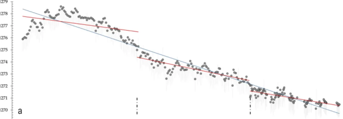
In order to analyse the time series of height above reference surface variations of lakes extracted from radar altimetry data, two models have been used. In the first model, the time series were treated as a whole under the hypothesis that the time series has a decreasing (blue lines in Figure7) trend in Urmia Lake and an increasing trend in Sevan and Van Lakes (Figure7). In the second model, by applying PELT algorithm, the time series have been divided into segments (black lines in Figure7) with its own statistical characteristics that are similar within each subseries and different between subseries. It seems that the increasing mono-trend (red lines in Figure7) fitted to the whole time series can have different behaviour when multiple inner trends are taken into account.
Water 2016, 8, 478 11 of 19
treated as a whole under the hypothesis that the time series has a decreasing (blue lines in Figure 7) trend in Urmia Lake and an increasing trend in Sevan and Van Lakes (Figure 7). In the second model, by applying PELT algorithm, the time series have been divided into segments (black lines in Figure 7) with its own statistical characteristics that are similar within each subseries and different between subseries. It seems that the increasing mono‐trend (red lines in Figure 7) fitted to the whole time series can have different behaviour when multiple inner trends are taken into account.
Figure 7. Time series of height above reference surface variations of: (a) Urmia Lake area between 1992 and 2011; (b) Lake Sevan area between 2002 and 2015; and (c) Van Lake area between 2002 and 2015 extracted from radar altimetry data.
Figure 7.Time series of height above reference surface variations of: (a) Urmia Lake area between 1992 and 2011; (b) Lake Sevan area between 2002 and 2015; and (c) Van Lake area between 2002 and 2015 extracted from radar altimetry data.
Water2016,8, 478 12 of 19
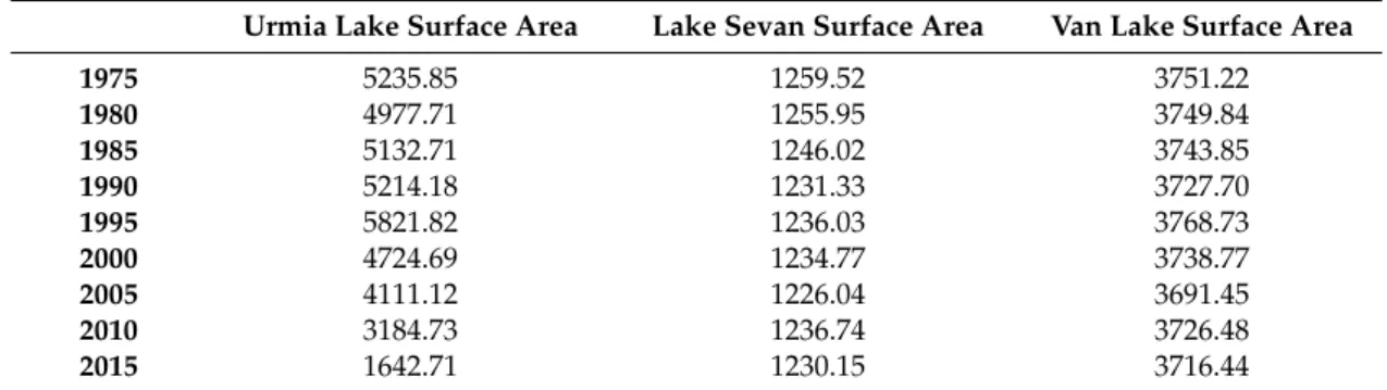
Table 3.The lakes surface area changes (km2) generated by MLP NNs classifier.
Urmia Lake Surface Area Lake Sevan Surface Area Van Lake Surface Area
1975 5235.85 1259.52 3751.22
1980 4977.71 1255.95 3749.84
1985 5132.71 1246.02 3743.85
1990 5214.18 1231.33 3727.70
1995 5821.82 1236.03 3768.73
2000 4724.69 1234.77 3738.77
2005 4111.12 1226.04 3691.45
2010 3184.73 1236.74 3726.48
2015 1642.71 1230.15 3716.44
The generated results revealed a significant change in the surface area of Urmia Lake. These changes confirm different natural and human-made external driving forces in the watershed area.
Investigations on the Urmia Lake water level breakpoints on 2000 and 2008 shows that the lake had experienced rapid changes in its history. These rapid changes could refer to intensive dam construction on one the hand and intensive and extensive cultivation activities by increasing the irrigation land on the other hand (Figures8and9). The above-mentioned changes from 2000 to 2015 have been confirmed by the surface area generated using MLP NNs classifier.
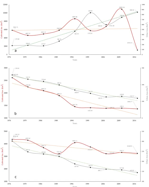
Moreover, monitoring the lake’s long term changes (Figure6) and comparing them with long term anthropogenic activities (e.g., land use change, land over use, dam construction and urbanization as it has been shown in Figure8) in the watershed area of the lake indicate that the unsustainable land management has been significantly impact in drying up the Urmia Lake as well.
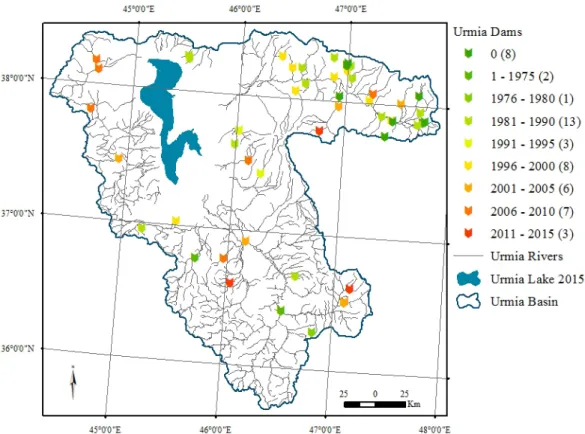
The results also show that with increasing the intensive human activities in different periods, the drying trend increased. For instance, there are 51 dams in Urmia Lake basin which have been constructed to supply irrigation demands (Figure9). Moreover, based on the authors knowledge, there are 224 projects (72 reservoir dams, 124 weirs and conduction facilities, 17 pumping stations and 10 flood controlling and artificial feeding) under study, 231 of which were assessed to be constructed in the near future [62]. The under construction projects regulate 1499.9 MCM water (under study projects regulate 657.2 MCM water). Therefore, total regulated water volume will be 3869.1 MCM within approximately 20 years [62].
Figure 9 shows the most important projects in this area. Long term climate change and perturbation enhanced the negative effects of mismanagement and caused critical condition for the Urmia Lake in the resent years. As it has been shown in Figure10, the annual average precipitation on Urmia Lake basin was 382.4 mm from 1966 to 1990, which has been decreased to 315.5 mm from 1991 to 2015. The temperature average over Urmia Lake basin was nearly 11.6◦C from 1966 to 1990 that has reached an average of 12◦C from 1991 to 2015.
Figure 8. Temporal land use changes (every five years) in the period 1975–2015 for: (a) Urmia Lake basin; (b) Lake Sevan basin; and (c) Van Lake basin.
Figure 8.Temporal land use changes (every five years) in the period 1975–2015 for: (a) Urmia Lake basin; (b) Lake Sevan basin; and (c) Van Lake basin.
Water2016,8, 478 14 of 19
Water 2016, 8, 478 14 of 19
Figure 9. The geographical locations of dams (grouped by the year of operation) over Lake Urmia basin.
Figure 10. Time series of annual Precipitation (mm) and Temperature (°C) for the Urmia Lake basin between 1966 and 2015.
6. Conclusions
In this study, a multisensory, multitemporal remote sensing approach has been used to monitor water level and storage variations of Urmia Lake, Lake Sevan, and Van Lake. In order to examine the proposed model, these three study areas have been selected because they are under intensive natural and human driving forces. Landsat TM, ETM+ and OLI multitemporal images and Topex/Poseidon, Jason‐1 and 2, and GFO satellite data have been used together with climate data to identify lake parameters (water level variations) and separate them from other land cover types (surface water extraction). The results show that, the Urmia Lake’s water level and area decrease at a significant rate, which is dramatically high in comparison with Lake Sevan and Van Lake.
Furthermore, an approach based on multilayer perceptron neural networks algorithm has been introduced for surface water change detection, which shows high performance in simultaneously detecting the surface water changes in comparison with the other state of the art models presented in
Figure 9.The geographical locations of dams (grouped by the year of operation) over Lake Urmia basin.
Water 2016, 8, 478 14 of 19
Figure 9. The geographical locations of dams (grouped by the year of operation) over Lake Urmia basin.
Figure 10. Time series of annual Precipitation (mm) and Temperature (°C) for the Urmia Lake basin between 1966 and 2015.
6. Conclusions
In this study, a multisensory, multitemporal remote sensing approach has been used to monitor water level and storage variations of Urmia Lake, Lake Sevan, and Van Lake. In order to examine the proposed model, these three study areas have been selected because they are under intensive natural and human driving forces. Landsat TM, ETM+ and OLI multitemporal images and Topex/Poseidon, Jason‐1 and 2, and GFO satellite data have been used together with climate data to identify lake parameters (water level variations) and separate them from other land cover types (surface water extraction). The results show that, the Urmia Lake’s water level and area decrease at a significant rate, which is dramatically high in comparison with Lake Sevan and Van Lake.
Furthermore, an approach based on multilayer perceptron neural networks algorithm has been introduced for surface water change detection, which shows high performance in simultaneously detecting the surface water changes in comparison with the other state of the art models presented in
Figure 10.Time series of annual Precipitation (mm) and Temperature (◦C) for the Urmia Lake basin between 1966 and 2015.
6. Conclusions
In this study, a multisensory, multitemporal remote sensing approach has been used to monitor water level and storage variations of Urmia Lake, Lake Sevan, and Van Lake. In order to examine the proposed model, these three study areas have been selected because they are under intensive natural and human driving forces. Landsat TM, ETM+ and OLI multitemporal images and Topex/Poseidon, Jason-1 and 2, and GFO satellite data have been used together with climate data to identify lake parameters (water level variations) and separate them from other land cover types (surface water extraction). The results show that, the Urmia Lake’s water level and area decrease at a significant rate, which is dramatically high in comparison with Lake Sevan and Van Lake.
Furthermore, an approach based on multilayer perceptron neural networks algorithm has been introduced for surface water change detection, which shows high performance in simultaneously detecting the surface water changes in comparison with the other state of the art models presented in the related literature. In conclusion, the proposed model (as a global model which can be applied to another datasets just with some parameter adjustments based on the type of data) has been proven to be effective in detecting the water surface changes in different lakes. The construction of the NN model can be a time consuming process (which is considered as the weakness of the model in comparison with the other algorithms) since building up the NN architecture is synonymous to a strenuous activity involving trial and error.
Then, the impact of factors such as climate change (e.g., rain variation) and anthropogenic activities (e.g., dam construction and water overuse) have been demonstrated. The results show that despite the long-term transformation of the environment by human activities as well as climate change in the watershed area of the three lakes, Lake Urmia is in critical situation and urgent action is needed for the lake to survive. It can be concluded that construction of dams in Urmia Lake basin was not the main factor in declining the lake level but the drying up of Urmia Lake has been occurred due to a chain of reasons, which are highly influenced by anthropogenic activities and climate change.
Managing water supply and irrigation, strict water rights, and modifying farming to conserve water and averting new dam construction in the basin are suggested to help Urmia Lake to make a recovery. However, continuous time series of temperature, precipitation and other meteorological observations and estimations (e.g., evaporation and aridification) on the lake and in the watershed, as well as of the discharge of surface water to the lake would help to better constrain the water balance.
Acknowledgments:The paper has been financed by Land Schleswig-Holstein within the funding programme Open Access Publikationsfonds.
Author Contributions: Model development, the experiments conceive, design and perform have been done by Alireza Taravat and Iraj Emadodin. Data analyses have been done by Alireza Taravat, Masih Rajaei, Hamidreza Hasheminejad, and Rahman Mousavian. Paper writing and correction have been done by Alireza Taravat and Masih Rajaei. Ehsan Biniyaz has improved the grammar and readability of the paper.
Conflicts of Interest:The authors declare no conflict of interest.
References
1. Zhu, W.; Jia, S.; Lv, A. Monitoring the fluctuation of Lake Qinghai using multi-source remote sensing data.
Remote Sens.2014,6, 10457–10482. [CrossRef]
2. Daily, G.Nature’s Services: Societal Dependence on Natural Ecosystems; Island Press: Washington, DC, USA, 1997; p. 329.
3. Ozesmi, S.L.; Bauer, M.E. Satellite remote sensing of wetlands. Wetl. Ecol. Manag. 2002, 10, 381–402.
[CrossRef]
4. Crétaux, J.-F.; Jelinski, W.; Calmant, S.; Kouraev, A.; Vuglinski, V.; Bergé-Nguyen, M.; Gennero, M.-C.;
Nino, F.; Del Rio, R.A.; Cazenave, A. Sols: A lake database to monitor in the near real time water level and storage variations from remote sensing data.Adv. Space Res.2011,47, 1497–1507. [CrossRef]
5. Alsdorf, D.E.; Rodriguez, E.; Lettenmaier, D.P. Measuring surface water from space.Rev. Geophys.2007,45.
[CrossRef]
6. Calmant, S.; Seyler, F.; Cretaux, J.F. Monitoring continental surface waters by satellite altimetry.Surv. Geophys.
2008,29, 247–269. [CrossRef]
7. Frappart, F.; Calmant, S.; Cauhopé, M.; Seyler, F.; Cazenave, A. Preliminary results of ENVISAT RA-2-derived water levels validation over the Amazon basin.Remote Sens. Environ.2006,100, 252–264. [CrossRef]
8. Duan, Z.; Bastiaanssen, W. Estimating water volume variations in lakes and reservoirs from four operational satellite altimetry databases and satellite imagery data.Remote Sens. Environ.2013,134, 403–416. [CrossRef]
9. Medina, C.E.; Gomez-Enri, J.; Alonso, J.J.; Villares, P. Water level fluctuations derived from ENVISAT Radar Altimeter (RA-2) and in-situ measurements in a subtropical waterbody: Lake Izabal (Guatemala).
Remote Sens. Environ.2008,112, 3604–3617. [CrossRef]
Water2016,8, 478 16 of 19
10. Zhang, J.; Xu, K.; Yang, Y.; Qi, L.; Hayashi, S.; Watanabe, M. Measuring water storage fluctuations in Lake Dongting, China, by Topex/Poseidon satellite altimetry.Environ. Monit. Assess.2006,115, 23–37. [CrossRef]
[PubMed]
11. Crétaux, J.-F.; Birkett, C. Lake studies from satellite radar altimetry. C. R. Geosci. 2006, 338, 1098–1112.
[CrossRef]
12. Demir, B.; Bovolo, F.; Bruzzone, L. Updating land-cover maps by classification of image time series: A novel change-detection-driven transfer learning approach. IEEE Trans. Geosci. Remote Sens. 2013,51, 300–312.
[CrossRef]
13. Salmon, B.P.; Kleynhans, W.; van den Bergh, F.; Olivier, J.C.; Grobler, T.L.; Wessels, K.J. Land cover change detection using the internal covariance matrix of the extended Kalman filter over multiple spectral bands.
IEEE J. Sel. Top. Appl. Earth Obs. Remote Sens.2013,6, 1079–1085. [CrossRef]
14. Brisco, B.; Schmitt, A.; Murnaghan, K.; Kaya, S.; Roth, A. SAR polarimetric change detection for flooded vegetation.Int. J. Digit. Earth2013,6, 103–114. [CrossRef]
15. Volpi, M.; Petropoulos, G.P.; Kanevski, M. Flooding extent cartography with Landsat TM imagery and regularized kernel fisher’s discriminant analysis.Comput. Geosci.2013,57, 24–31. [CrossRef]
16. Kaliraj, S.; Meenakshi, S.M.; Malar, V. Application of remote sensing in detection of forest cover changes using geo-statistical change detection matrices—A case study of Devanampatti reserve forest, Tamilnadu, India.Nat. Environ. Pollut. Technol.2012,11, 261–269.
17. Markogianni, V.; Dimitriou, E.; Kalivas, D. Land-use and vegetation change detection in plastira artificial lake catchment (Greece) by using remote-sensing and GIS techniques.Int. J. Remote Sens.2013,34, 1265–1281.
[CrossRef]
18. Bagan, H.; Yamagata, Y. Landsat analysis of urban growth: How Tokyo became the world’s largest megacity during the last 40 years.Remote Sens. Environ.2012,127, 210–222. [CrossRef]
19. Raja, R.A.; Anand, V.; Kumar, A.S.; Maithani, S.; Kumar, V.A. Wavelet based post classification change detection technique for urban growth monitoring.J. Indian Soc. Remote Sens.2013,41, 35–43. [CrossRef]
20. Dronova, I.; Gong, P.; Wang, L. Object-based analysis and change detection of major wetland cover types and their classification uncertainty during the low water period at Poyang lake, China.Remote Sens. Environ.
2011,115, 3220–3236. [CrossRef]
21. Zhu, X.; Cao, J.; Dai, Y. A decision tree model for meteorological disasters grade evaluation of flood.
In Proceedings of the 2011 Fourth International Joint Conference on Computational Sciences and Optimization (CSO), Kunming and Lijiang, China, 15–19 April 2011; IEEE: Piscataway, NJ, USA, 2011;
pp. 916–919.
22. Calvet, J.-C.; Wigneron, J.-P.; Walker, J.; Karbou, F.; Chanzy, A.; Albergel, C. Sensitivity of passive microwave observations to soil moisture and vegetation water content: L-band to w-band. IEEE Trans. Geosci.
Remote Sens.2011,49, 1190–1199. [CrossRef]
23. Desmet, P.; Govers, G. A GIS procedure for automatically calculating the USLE LS factor on topographically complex landscape units.J. Soil Water Conserv.1996,51, 427–433.
24. Du, Z.; Linghu, B.; Ling, F.; Li, W.; Tian, W.; Wang, H.; Gui, Y.; Sun, B.; Zhang, X. Estimating surface water area changes using time-series Landsat data in the Qingjiang River Basin, China.J. Appl. Remote Sens.2012, 6, 063609. [CrossRef]
25. Sun, F.; Sun, W.; Chen, J.; Gong, P. Comparison and improvement of methods for identifying waterbodies in remotely sensed imagery.Int. J. Remote Sens.2012,33, 6854–6875. [CrossRef]
26. Bai, J.; Chen, X.; Li, J.; Yang, L.; Fang, H. Changes in the area of inland lakes in arid regions of central Asia during the past 30 years.Environ. Monit. Assess.2011,178, 247–256. [CrossRef] [PubMed]
27. Jawak, S.D.; Kulkarni, K.; Luis, A.J. A review on extraction of lakes from remotely sensed optical satellite data with a special focus on cryospheric lakes.Adv. Remote Sens.2015,4, 196–213. [CrossRef]
28. Mason, I.; Guzkowska, M.; Rapley, C.; Street-Perrott, F. The response of lake levels and areas to climatic change.Clim. Chang.1994,27, 161–197. [CrossRef]
29. Goerner, A.; Jolie, E.; Gloaguen, R. Non-climatic growth of the saline Lake Beseka, Main Ethiopian Rift.
J. Arid Environ.2009,73, 287–295. [CrossRef]
30. Mercier, F.; Cazenave, A.; Maheu, C. Interannual lake level fluctuations (1993–1999) in Africa from Topex/Poseidon: Connections with ocean–atmosphere interactions over the Indian Ocean.
Glob. Planet. Chang.2002,32, 141–163. [CrossRef]
31. Tourian, M.; Elmi, O.; Chen, Q.; Devaraju, B.; Roohi, S.; Sneeuw, N. A spaceborne multisensor approach to monitor the desiccation of Lake Urmia in Iran.Remote Sens. Environ.2015,156, 349–360. [CrossRef]
32. Birkett, C. The contribution of topex/poseidon to the global monitoring of climatically sensitive lakes.
J. Geophys. Res. Oceans1995,100, 25179–25204. [CrossRef]
33. Frappart, F.; Seyler, F.; Martinez, J.-M.; Leon, J.G.; Cazenave, A. Floodplain water storage in the Negro river basin estimated from microwave remote sensing of inundation area and water levels.Remote Sens. Environ.
2005,99, 387–399. [CrossRef]
34. Baup, F.; Frappart, F.; Maubant, J. Combining high-resolution satellite images and altimetry to estimate the volume of small lakes.Hydrol. Earth Syst. Sci.2014,18, 2007–2020. [CrossRef]
35. Frappart, F.; Papa, F.; Güntner, A.; Werth, S.; Da Silva, J.S.; Tomasella, J.; Seyler, F.; Prigent, C.; Rossow, W.B.;
Calmant, S. Satellite-based estimates of groundwater storage variations in large drainage basins with extensive floodplains.Remote Sens. Environ.2011,115, 1588–1594. [CrossRef]
36. Ramillien, G.; Frappart, F.; Seoane, L. Application of the regional water mass variations from grace satellite gravimetry to large-scale water management in Africa.Remote Sens.2014,6, 7379–7405. [CrossRef]
37. Singh, A.; Seitz, F.; Schwatke, C. Inter-annual water storage changes in the Aral Sea from multi-mission satellite altimetry, optical remote sensing, and GRACE satellite gravimetry.Remote Sens. Environ.2012,123, 187–195. [CrossRef]
38. Yan, L.-J.; Qi, W. Lakes in Tibetan Plateau extraction from remote sensing and their dynamic changes.
Acta Geosci. Sin.2012,33, 65–74.
39. Jensen, J.R.Remote Sensing of the Environment: An Earth Resource Perspective 2/e; Pearson Education: Delhi, India, 2009; pp. 15–17.
40. Song, C.; Huang, B.; Ke, L. Modeling and analysis of lake water storage changes on the Tibetan Plateau using multi-mission satellite data.Remote Sens. Environ.2013,135, 25–35. [CrossRef]
41. Rokni, K.; Ahmad, A.; Selamat, A.; Hazini, S. Water feature extraction and change detection using multitemporal Landsat imagery.Remote Sens.2014,6, 4173–4189. [CrossRef]
42. Xu, H. Modification of normalised difference water index (NDWI) to enhance open water features in remotely sensed imagery.Int. J. Remote Sens.2006,27, 3025–3033. [CrossRef]
43. Ouma, Y.O.; Tateishi, R. A water index for rapid mapping of shoreline changes of five East African Rift Valley lakes: An empirical analysis using Landsat TM and ETM+ data. Int. J. Remote Sens.2006,27, 3153–3181.
[CrossRef]
44. Frazier, P.S.; Page, K.J. Water body detection and delineation with Landsat TM data. Photogramm. Eng.
Remote Sens.2000,66, 1461–1468.
45. Soh, L.-K.; Tsatsoulis, C. Segmentation of satellite imagery of natural scenes using data mining.IEEE Trans.
Geosci. Remote Sens.1999,37, 1086–1099.
46. Alecu, C.; Oancea, S.; Bryant, E. Multi-resolution analysis of MODIS and ASTER satellite data for water classification. In Proceedings of the Remote Sensing for Environmental Monitoring, GIS Applications, and Geology, Bruges, Belgium, 19 September 2005; International Society for Optics and Photonics: Bellingham, WA, USA, 2005; p. 59831Z.
47. Zhang, Y.; Pulliainen, J.T.; Koponen, S.S.; Hallikainen, M.T. Water quality retrievals from combined Landsat TM data and ERS-2 SAR data in the Gulf of Finland.IEEE Trans. Geosci. Remote Sens. 2003,41, 622–629.
[CrossRef]
48. Yang, K.; Smith, L.C. Supraglacial streams on the Greenland ice sheet delineated from combined spectral–shape information in high-resolution satellite imagery. IEEE Geosci. Remote Sens. Lett. 2013, 10, 801–805. [CrossRef]
49. Jawak, S.D.; Luis, A.J. Improved land cover mapping using high resolution multiangle 8-band WorldView-2 satellite remote sensing data.J. Appl. Remote Sens.2013,7, 073573. [CrossRef]
50. Shao, P.; Yang, G.; Niu, X.; Zhang, X.; Zhan, F.; Tang, T. Information extraction of high-resolution remotely sensed image based on multiresolution segmentation.Sustainability2014,6, 5300–5310. [CrossRef]
51. Jeon, Y.-J.; Choi, J.-G.; Kim, J.-I. A study on supervised classification of remote sensing satellite image by bayesian algorithm using average fuzzy intracluster distance. InInternational Workshop on Combinatorial Image Analysis; Klette, R., Žuni´c, J., Eds.; Springer: Berlin/Heidelberg, Germany, 2004; pp. 597–606.
52. McFeeters, S.K. The use of the normalized difference water index (NDWI) in the delineation of open water features.Int. J. Remote Sens.1996,17, 1425–1432. [CrossRef]