Interannual Variability of Tropical Pacific Sea Level from 1993 to 2014
Xiaoting Zhu,1 Richard J. Greatbatch,1,2 and Martin Claus1
Corresponding author: Xiaoting Zhu, GEOMAR Helmholtz Centre for Ocean Research Kiel, Kiel, Germany. (xzhu@geomar.de)
1GEOMAR Helmholtz Centre for Ocean Research Kiel, Kiel, Germany.
2Faculty of Mathematics and Natural Sciences, University of Kiel, Kiel, Germany.
DOI 10.1002/2016JC012347
Abstract.
A multi-mode, linear reduced-gravity model, driven by ERA-Interim monthly mean wind stress anomalies, is used to investigate interannual variability in tropical Pacific sea level as seen in satellite altimeter data. The model out- put is fitted to the altimeter data along the equator, in order to derive the vertical profile for the model forcing, showing that a signature from modes higher than mode six cannot be extracted from the altimeter data. It is shown that the model has considerable skill at capturing interannual sea level vari- ability both on and off the equator. The correlation between modelled and satellite-derived sea level data exceeds 0.8 over a wide range of longitudes along the equator and readily captures the observed ENSO events. Overall, the combination of the first, second, third and fifth modes can provide a ro- bust estimate of the interannual sea level variability, the second mode be- ing dominant. A remarkable feature of both the model and the altimeter data is the presence of a pivot point in the western Pacific on the equator. We show that the westward displacement of the pivot point from the centre of the basin is strongly influenced by the fact that most of the wind stress variance is found in the western part of the basin. We also show that the Sverdrup transport is not fundamental to the dynamics of the recharge/discharge mechanism in our model, although the spatial structure of the wind forcing does play a role in setting the amplitude of the “warm water volume”.
1. Introduction
More than 40 years ago, interannual sea level variability in the tropical Pacific was being studied using linear, reduced-gravity models driven by estimates of the observed surface wind stress [Busalacchi and O’Brien, 1981;Busalacchi et al., 1983]. At that time, the only available sea level data was from the sparse tide gauge record. However, with the advent of satellite data, there has been a revolution in the available data coverage for sea level. Here, we revisit the ability of linear models to capture interannual variability in tropical Pacific sea level, this time using a multi-mode modelling system and taking advantage of the tem- porally and spatially comprehensive altimetric sea level data produced by Ssalto/Duacs and distributed by Aviso with support from Cnes (http://www.aviso.altimetry.fr/duacs/).
In the tropical Pacific, interannual variability is dominated by the El Ni˜no-Southern Oscillation (ENSO) phenomenum, with widespread environmental impacts locally, but also around the world due to the global teleconnections in the ocean and the atmosphere [Philander, 1989;Trenberth et al., 1998]. Observational studies [e.g. Delcroix, 1998;For- get and Ponte, 2015] have shown that sea level variations associated with ENSO feature an east-west contrast along the equator and zonally uniform anomalies near the equator.
These features are also captured by analytical solutions for the linear response of the trop- ical Pacific Ocean to low-frequency wind forcing [Clarke, 2010], where they correspond to what Clarke calls the “tilt” mode and “equatorial warm water volume (WWV)”, respec- tively (see Meinen and McPhaden [2000] and Meinen and McPhaden [2001] for an early discussion of these modes). According to Clarke [2010], the tilt mode is a quasi-steady response to wind forcing that varies in phase with the wind stress forcing, i.e. the bal-
ance of the zonal wind stress by the zonal pressure gradient; however, the WWV mode lags the wind stress due to the strong dependence of the westward propagation speed for long Rossby waves on latitude. The phase lag is a key feature of the recharge/discharge mechanism for ENSO [Jin, 1997] as reviewed by Neelin et al. [1998].
The early studies in the 1970’s and 1980’s suggested an important role for Kelvin and Rossby waves in the dynamics of the tropical oceans and, indeed, in the dynamics of ENSO. Recent work has confirmed that the interannual variability of sea level at low latitudes is almost exclusively baroclinic in origin [Forget and Ponte, 2015]. Large-scale, low-frequency (interannual) oceanic motion can be separated into an infinite number of baroclinic vertical normal modes [Gill and Clarke, 1974;Gill, 1982], of which the first few modes usually dominate. Moon et al. [2004] claimed that interannual variations in the relative importance of different vertical wave modes is important for the predictability of ENSO and Dewitte et al. [1999] analysed the contributions of the first four baroclinic modes to sea level variability for the period 1985-1994 using an ocean general circulation model. The authors found that the first-mode is most dominant in the western Pacific and the second-mode in the eastern Pacific. Other authors have also noted the dominance of the first and second modes [Cane, 1984; Busalacchi and Cane, 1985; Yu and McPhaden, 1999; McPhaden and Yu, 1999].
Nevertheless, the relative importance of the different vertical modes is still not ad- equately explored. To provide more information about the relative importance of the different baroclinic modes for explaining the interannual variability of sea level in the tropical Pacific Ocean, we conduct simulations using a multi-mode modelling system. We assign the weighting to each mode with the help of altimeter data without assuming, a
priori, the vertical profile in the ocean for the wind-induced forcing, different from previ- ous studies [Gill and Clarke, 1974; Cane, 1984; Dewitte et al., 1999]. In particular, we fit the model results to the altimetric measurements along the equator in order to diagnose the projection coefficients for each mode for the vertical profile of the model forcing.
Clarke [2010] argues that the origin of the disequilibrium WWV mode is the strong dependence of the propagation speed for long Rossby waves on latitude. On the other hand, in the original recharge/discharge theory put forward by [Jin, 1997], an important role was assigned to the Sverdrup transport for transferring mass to and from the equator.
We address the role of the Sverdrup transport in our model using spatially uniform wind stress forcing given by the time series of the zonally-averaged zonal wind stress along the equator, for which the Sverdrup transport is zero.
The paper is organized as follows. The description of the model and the methods employed are outlined in the Section 2. Section 3 shows the results and discusses the recharge/discharge mechanism using the model. Finally, Section 4 summarises the main conclusions.
2. Methods
2.1. Basic equations
Our starting point is the Boussinesq, hydrostatic equations for a continuously stratified ocean linearized about a state of rest. In spherical coordinates, these are given by
∂u
∂t −f v=− 1 ρoacosθ
∂p′
∂λ + τsx
ρoHEG(z) +Fu (1)
∂v
∂t +f u=− 1 ρoa
∂p′
∂θ + τsy ρoHE
G(z) +Fv (2)
0 =−∂p′
∂z −gρ′ (3)
1 acosθ[∂u
∂λ + ∂(vcosθ)
∂θ ] + ∂w
∂z = 0 (4)
∂ρ′
∂t +w∂ρ
∂z = 0 (5)
whereθ is latitude,λ is longitude,ais the radius of the Earth,f = 2Ω sinθis the Coriolis parameter, g is the gravitational acceleration, ρo a representative density for sea water, u, v, w are the velocity components in the eastward, northward and vertically upward directions, respectively, ρ′ is the density perturbation,p′ is the pressure perturbation, (τsx, τsy) is the surface wind stress treated as a body force with a vertical structure G(z), HE is a depth scale for the surface Ekman layer (here independent of both space and time), and Fu,Fv is the lateral mixing of momentum with horizontal eddy viscosity coefficient, Ah, given by
Fu(u, v) = Ah a2
[ 1 cos2θ
∂2u
∂λ2 + 1 cosθ
∂
∂θ
(
cosθ∂u
∂θ
)
+u(1−tan2θ)−2 sinθ cos2θ
∂v
∂λ
]
(6)
Fv(u, v) = Ah
a2
[ 1 cos2θ
∂2v
∂λ2 + 1 cosθ
∂
∂θ
(
cosθ∂v
∂θ
)
+v(1−tan2θ)−2 sinθ cos2θ
∂u
∂λ
]
. (7)
The boundary conditions are, at the surface z = 0,
p′ =ρogη and w= ∂η∂t (8)
where η denotes the sea level anomaly, and at the bottom z = −H, w = 0, where H is the total depth of the ocean (assumed here to be flat).
As is well known, the solution to these equations can be expressed as the superposition of a infinite discrete set of vertical normal modes [Gill and Clarke, 1974; Gill, 1982], so that the pressure perturbation p′, for example, can be expressed as
p′ ρog =
∑∞ n=1
ˆ
pn(z)ηn(λ, θ, t) (9)
where the subscript n refers to the nth normal mode, ˆpn(z) denotes the corresponding normalized vertical structure function for pressure satisfying ∫−0Hpˆ2n(z)dz = 1, and the horizontal structure associated with each vertical mode is obtained by solving the shallow water equations
∂un
∂t −f vn=− g acosθ
∂ηn
∂λ + τsx
ρHEGn+Fnu (10)
∂vn
∂t +f un=−g a
∂ηn
∂θ + τsy
ρHEGn+Fnv (11)
∂ηn
∂t + Hn acosθ
[∂un
∂λ + ∂(cosθvn)
∂θ
]
= 0. (12)
Here repeated variables are consistent with those in Eqs. (1)-(5), except for the subscript n referring to the nth normal mode, Hn is the equivalent depth determined by the wave speed cn = √
gHn, and Gn = ∫−H0 G(z)ˆpn(z)dz is the wind forcing profile projection factor. The sea surface height anomaly, which is to be compared to that from the satellite altimeter, is then given by
η=
∑∞ n=1
ˆ
pn(0)ηn(λ, θ, t). (13)
Here, we do not specify the vertical profile of the wind forcing, G(z), a priori and first solve these equations withGn = 1 to obtain a corresponding field forηn which we denote as ηn∗, excluding the barotropic mode (n = 0). We then make a least squares fit of the model-computed sea level anomalies to the sea level anomalies from the altimeter data.
The fit is carried out along the equator across the whole of the equatorial Pacific, to obtain fitting coefficients γn for each mode. The model-computed sea level is then given by
η=
∑N
n=1
γnpˆn(0)ηn∗(λ, θ, t) (14)
where N is the number of modes used for the fit. The implied projection coefficients, Gn
are given by
Gn=γn (15)
and the vertical profile for the wind forcing can then be obtained from
G(z) =
∑N
n=1
ˆ
pn(z)γn. (16)
2.2. Model setup
The model domain extends from 112◦E to 70◦W zonally and from 12◦S to 18◦N merid- ionally, similar to that of Busalacchi and O’Brien [1981], with the 300 m isobath taken as the coastline, and the horizontal resolution is 0.5◦ in latitude and longitude. The east- ern/western boundaries are treated as solid walls. Sponge layers, damping the velocity field only, with e-folding scale of 5◦ in latitude, are applied to the northern and southern boundaries to eliminate wave propagation along those boundaries. The scale depth HE
is chosen to be 300 m and the eddy viscosity coefficient Ah is 5000 m2 s−1 everywhere1 Monthly mean wind stress anomalies from January 1979 to September 2014 are used to force the model. Anomalies are computed relative to the climatological monthly mean for each month for the period 1993 to 2012 and are derived from ERA-interim monthly mean wind stress provided by the European Centre for Medium-Range Weather Fore- casts (ECMWF) [Berrisford et al., 2009]. The satellite measured sea level anomalies from January 1993 to September 2014 are those produced by Ssalto/Duacs and distributed by Aviso with support from Cnes (http://www.aviso.altimetry.fr/duacs/).
To derive the vertical normal modes, the vertical profile of the buoyancy frequency is
and salinity data from the World Ocean Atlas 2013 dataset [Locarnini et al., 2013]. The resulting profiles are then averaged to produce an averaged buoyancy frequency profile within the model domain. The averaged buoyancy frequency profile is then used to com- pute the vertical modes. The resulting wave speeds of the first five baroclinic modes are 2.88, 1.72, 1.10, 0.82 and 0.67 m s−1, respectively, and the corresponding vertical structure functions, ˆpn(z), are shown in Figure 1a. The horizontal resolution of 0.5◦ in latitude and longitude is sufficient to resolve the equatorial baroclinic Rossby radius of deformation
√c
β for the selected normal modes, where β is the latitudinal gradient of the Coriolis parameter given by β = 2Ωcos(θ)a .
Two additional model experiments are carried out using exactly the same setup as above. In the first (referred to as experiment ZMW), the meridional wind stress is set to zero and the zonal wind stress is spatially uniform over the model domain. In this experiment, the zonal wind stress is given by the time series of the zonal average along the equator of the zonal wind stress anomalies from the standard experiment; that is from ERA-Interim. In the second, the meridional wind stress is again zero but the zonal wind stress is given by the time series of the zonal mean zonal wind stress at each latitude (referred to as experiment LatZM). The vertical profile for the model forcing in both these experiments is the same as in the standard run. In experiment ZMW, because the wind stress is spatially uniform, the Sverdrup transport is zero.
3. Results
As described in Section 2, the vertical structure of the wind forcing profile, given by G(z) in equations (1) and (2), is deduced from the model solution by fitting monthly mean anomalies of the model sea level to the AVISO data along the equator. The coefficients
Gn (see eqns. (15) and (16)) obtained from the fitting, and using increasing numbers of vertical modes, are shown in Table 1. It is clear that the weighting assigned to modes 1 and 2 is quite stable once 3 or more modes are used. However, increasing the number of modes from 4 to 5 reduces the weighting given to mode 4 and puts more weight into modes 3 and 5. Adding a sixth mode does not change this picture but using 7 modes or more leads to the appearance of large weightings that largely cancel out. This behaviour is an indication that beyond mode 6, it is no longer possible to separate the signature of the modes in the AVISO data. Equation (16) can be used to construct the wind forcing profile, as shown in Figure 1b when using 5 modes and when using 4 and 6 modes in Figure 1c. In all cases, the profile is strongly surface intensified, as one would expect, but with a clear improvement in going from 4 to 5 or 6 modes. Note, in particular, the reduced amplitude below 200 m depth when using 5 or 6 modes and also that there is little change in going from 5 to 6 modes. Clearly, further reducing the amplitude below 200 m depth would require an accurate estimate of γn for modes higher than 6, something that is not possible through fitting our model solutions to the altimeter data. Since adding the sixth mode makes very little contribution to our results (the coefficient γ6 is close to zero) we work with 5 modes in what follows.
Before leaving Table 1, it is worth commenting on the weighting when using 5 modes.
Note, in particular, the dominance of mode 2 but also that some role is given to mode 3, followed by modes 1 and 5, with the smallest weighting being given to mode 4. These weightings assign the amplitude that is given to the forcing for each mode in equations (10) and (11), with Gn =γn (equation (15)). It is, therefore, no surprise that the second mode dominates our results, although with some role for modes 1,3 and 5, as we shall
see. There are two reasons for favouring mode 5 over mode 4. The first is the consistency between the weightings attached to each mode when going from 5 to 6 modes to make the fit (see Table 1). The second is the improved vertical structure of the wind forcing profile shown in Figure 1 when using 5 or 6 modes as distinct from 4 modes, a point already noted above. Nevertheless, whether or not the fitting is really able to distingush between the 4th and 5th modes is a moot point, given that the difference in the gravity wave speeds for the two modes is only 0.15 m s−1. Another concern is the impact of the mean flow on the modes, an issue discussed by McPhaden et al. [1986] who note that the higher the mode, the more likely is an impact from the background flow. On the other hand, as shown by Brandt et al. [2016], mode 4 plays a role in the annual cycle of the equatorial Atlantic and is well represented by dynamics linearised about a state of rest. Regarding the dominance of mode 2 in the tropical ocean, this was already pointed out by Philander and Pacanowski [1980] and is discussed in detail there. We believe the difference between our results and previous studies, in particular Cane [1984],Busalacchi and Cane [1985], Yu and McPhaden [1999] and McPhaden and Yu [1999], is that we do not assume a vertical structure for the model forcing a priori, rather determining it by fitting the model to the AVISO data. We note that the common practice in previous studies, e.g. Cane [1984], has been to assume that the vertical structure functionG(z) in equations (1) and (2) is equal toHE/D over a surface Ekman layer of depthDand is zero below. Table 2 shows the projection coefficientsGnin this case for different choices of the depth D. These projection coefficients can be compared directly to those shown in Table 1. It is immediately apparent that the first mode now has a similar weight to that given to the second mode and also that less weight is given to the higher modes (apart from the
case with the shallowest D, i.e. D= 50m), consistent with the relative weightings of the modes found in previous studies. The different weightings given to the modes in our case therefore follows directly from the freedom we give our model to determine the vertical structure functionG(z) by fitting to the altimeter data. It is also interesting to note that if the depth D were to vary in time (as one would expect in a more realistic model) then one would expect the transition at the base of the Ekman layer to be smoothed out and look something like our derived vertical profile shown in Figure 1.
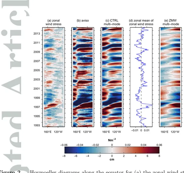
The Hovmoeller diagrams of monthly mean sea level anomalies along the equator (Fig.
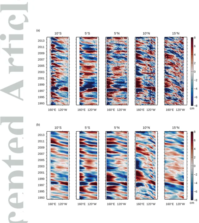
2c) and higher latitudes (Fig. 3b) exhibit remarkably similar patterns as those seen in the altimetric observations (Fig. 2b and 3a), illustrating the practical value of regarding the wind forcing as the null hypothesis for the origin of interannual sea level variability over the tropical Pacific. In particular, the model successfully captures the ENSO events of various strengths and flavours, including both conventional El Ni˜no (97/98, 06/07, 09/10) and Modoki El Ni˜no (94/95, 02/03, 04/05, i.e., positive anomalous sea levels do not extend to the eastern boundaries) [Ashok et al., 2007] events as well as the 95/96, 98/99, 07/08, 10/11 La Ni˜na events. Along the equator (Fig. 2b and 2c), El Ni˜no events are featured by positive anomalous sea level in the east and negative in the west, and vica versa during La Ni˜na events. The features, especially during the strong 97/98 El Ni˜no and 98/99 La Ni˜na, extend to other latitudes (Fig. 3a and 3b), by means of Kelvin wave propagation along the eastern boundary and subsequent Rossby wave propagation into the basin interior. This is in accordance with inferences from the observed surface dynamic height anomaly made, for example, by Delcroix [1998].
In contrast to the typically eastward propagation along the equator (Figure 2), events away from the equator generally propagate westwards (Figure 3). The propagation speeds along 10◦S, 5◦S, 5◦N and 10◦N in the model (Figure 3b) are comparable to those in the observations (Figure 3a), although at 15◦N, the modelled propagation speeds seem higher, even though many of the same events are seen in both the observations and the model.
A notable feature of both the model and the observations is an underlying symmetry about the equator, which though not perfect, reflects the importance of the equatorial regions for generating off-equatorial anomalies, be that by direct wind forcing or by wave propagation processes, as described above.
Another notable feature along the equator (Figure 2) is the presence of a pivot point in the western equatorial Pacific where anomalies tend to change sign and the variability is notably reduced. The pivot point tends to be further west in the observations than in the model, no doubt reflecting processes missing from our linear model set-up (e.g. zonal advection processes along the equator that are known to be important in the western, central Pacific, e.g. Dewitte et al. [2013]). Comparing Figures 2c and 2e, it is clear that the spatial structure of the wind forcing matters for the location of the pivot point. In the Figure 2e, the wind forcing is purely zonal and spatially uniform and is given by the time series of the zonal mean of the anomalous zonal wind stress along the equator shown in Figure 2d. While it is notable that this experiment captures the same events as the standard experiment (Figure 2b), the pivot point in this experiment is less distinct and is shifted eastwards. Looking at Figure 2a, we can see that in reality, most of the variability in the zonal wind stress along the equator is found in the western part of the basin. If the wind stress anomalies are always close to being in equilibrium with the anomalous zonal
gradient of sea level along the equator, as implied by the “tilt” mode of Clarke [2010], then we would expect the pivot point to the shifted westward in Figure 2c compared to Figure 2e so that it coincides with the region where the variability in the zonal wind stress is highest. That the pivot point tends to be shifted westward from the centre of the basin even in Figure 2e is an indication that the recharge/discharge mechanism is operating in our model, an issue discussed further later.
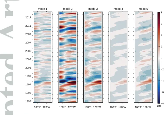
Figure 4 shows the contribution to model sea level from each of the five modes. The dominance of the second mode is immediately apparent. Modes 3 and 5, nevertheless, have a role to play; this can be seen most clearly during the major El Ni˜no events of 1997/98 and 2009/10, the largest amplitude events in the wind forcing time series. The same conclusion applies if we redraw Figure 4, but this time for the model run shown in Figure 2e that uses spatially uniform wind stress (not shown), implying that the spatial structure of the wind stress is not important for determining the role played by the different modes along the equator. The importance of the second mode is also seen in Figure 5 where the standard deviation of the sea level variability associated with each model is plotted (note the different scale used for the plots for individual modes). Some role for mode 1 is apparent in the western Pacific, for mode 3 in both the western and eastern Pacific and for mode 5 in the eastern Pacific. The dominance of mode 2, even in the western Pacific, is in contrast to the findings ofDewitte et al.[1999] that mode 1 was, if anything, slightly more important that mode 2 in the west in their model study covering the period 1985-1994 (see also Doi et al. [2010] who make a similar claim). Comparing the full, multi-mode model with the AVISO data, it is clear that the amplitude of the variability captured by the model is similar to that seen in the observations in the equatorial region and to some
extent off the equator near the western and eastern boundaries, especially in the west.
However, it is also clear that the model lacks variability in off-equatorial latitudes, one possible reason being the lack of tropical instability waves in the model. Nevertheless, as we noted when discussing Figure 3, many of the events present in the AVISO data are also present in the model.
Figure 6 shows the correlation between the model results and altimetric measurements.
It should be noted that a high correlation does not necessarily imply good model perfor- mance since correlation contains no information about amplitude, something that should be borne in mind when interpreting the figure. In particular, mode 4 explains little am- plitude (Figure 5) but still shows skill with correlation comparable to mode 3. The multi- mode model (Fig. 6a) nevertheless shows high correlations exceeding 0.7 (red colouring) over wide regions, especially near the western and eastern boundaries as well as along the equator where correlations widely exceed 0.8. A notable exception is the reduced correla- tion near the date line along the equator that arises from the misplacement of the pivot point in the model, noted when discussing Figure 2. There is clearly a related band of reduced correlation that extends eastward from the date line as one moves off the equator that is suggestive of a discrepancy between the Rossby wave propagation speeds in the model and the observations, although how this is linked to the reduced correlation on the equator is not clear. This is also the region where the amplitude in the model is low compared to that in AVISO (Figure 5) suggesting the role of processes missing from the model. The longitudinal structure of the correlation along the equator resembles the results from the ocean general circulation model in Dewitte et al.[1999] (see their Figure 6), despite the fact the phase speed for each mode is zonally uniform in our model and
we are comparing our model sea level anomalies to observations, not to sea level from a model as they are doing. Indeed, it is an interesting point that our model, which uses zonally uniform gravity wave speeds for each mode, shows considerable success at the equator despite the along-equator variations in the gravity wave speeds derived from a normal mode analysis noted by Picaut and Sombardier [1993] and also by Dewitte et al.
[1999]. Interestingly, Dewitte et al. [1999] note a drop in the wave speed associated with the baroclinic modes in their model just to the west of the date line (see their Figure 7b).
Such a drop in wave speed may be a factor in the misplacement of the pivot point in our model and suggests a role for physical processes other than linear wave dynamics. As noted earlier, a possible candidate is zonal advection which is known to play a role in the western-central Pacific [Dewitte et al., 2013]. Advective processes may also play a role off the equator.
The correlation maps for each individual mode are shown in Figures 6b-f. It is clear that, overall, the multi-model (Figure 6a) shows better performance compared to any single mode, although mode 1 shows generally higher correlations between 5◦N and 10◦N.
Once again, the second mode comes closest to the performance of the multi-mode model.
Overall, the first two modes show the best performance amongst the modes in the off- equatorial Pacific (poleward of 5◦N/S), whereas the higher modes show high correlation in the equatorial region (5◦S-5◦N) where modes 3 and 5, in particular, have a role to play, as we noted when discussing Figures 4 and 5. The phase in the eastern equatorial Pacific is almost exclusively affected by mode 2, with modes 1, 4 and 5 playing relatively little role there, while in the west mode 1 becomes more prominent. In the central equatorial Pacific, the correlation maxima slightly shift westward when going from lower to higher modes
presumably related to the slower wave propagation speeds and the greater importance of local wind forcing.
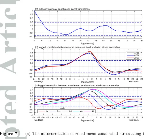
Finally, we can examine the recharge/discharge mechanism [Jin, 1997] using our model (see Neelin et al.[1998] for a review including discussion of the recharge/discharge mech- anism). As noted earlier, Clarke [2010] characterises interannual equatorial variability, such as associated with ENSO, with what he calls the “tilt”’ mode, in which the thermo- cline is tilted along the equator in quasi-equilibrium with the zonal wind forcing, and the warm water volume (WWV) associated with a net upward or downward displacement of the thermocline along the equator. Clarke [2010] argues that the existence of the WWV depends critically on the variation of the propagation speed for long Rossby waves with latitude and is not related to meridional divergence of the flow due to the wind forcing, as suggested, for example, in the original paper by Jin [1997] where an important role is assigned to the Sverdrup transport. We can investigate these modes in our model by looking at the correlation (see Figure 7) between ¯η, the zonal mean sea level along the equator, and the zonal mean of the zonal wind stress along the equator (referred to as
¯
τx hereafter) shown in Figure 2d. Here, ¯η is the signature of the WWV volume, being positive/negative when there is a greater volume of warm/cold water along the equator than in the mean.
First, Figure 7a shows the autocorrelation of ¯τx indicating a weak tendency for oscilla- tory behaviour with period of about 54 months (∼ 4.5 years) (the dashed blue lines, here, and also in Figures 7b,c indicate the 95% significance level). As can be seen from Fig.
7b, the correlation between ¯τx and ¯η from the standard multi-mode model agrees well with that from AVISO. The maximum negative correlation occurs at about 12 months
after the peak in the zonal mean zonal wind stress, implying that the WWV lags ¯τx by about 1 year or about a quarter cycle of the wind forcing after the wind stress maximum, in agreement with Clarke [2010]. In other words, roughly one year after a maximum in the eastward wind stress anomaly along the equator, the volume of warm water along the equator reaches a minimum, similar to what is shown in the schematic of Jin [1997], his Figure 1. For individual modes (Fig. 7c), the WWV of modes 1-5 lag ¯τx by about 5, 9, 14, 18 months and around 20 months (noting that there is no distinct minimum for mode 5), respectively. The increasing lag with mode number is an indication of the reduced wave speeds associated with the higher modes and, in particular, the reduced off-equatorial Rossby wave speeds leading to a slower off-equatorial adjustment, consistent with Clarke [2010]. Different from Figure 1 inJin [1997] is the positive correlation at lag 0 that arises when using sea level from both the multi-mode model and the AVISO data. It is this positive correlation that has a tendency to shift the pivot point, noted when discussing Figure 2, to the west. Assuming that the thermocline slope along the equator is always in equilibrium with the zonal wind stress (seeClarke[2010]), then when the anomalous zonal mean zonal wind stress is eastward (westward), the thermocline will be relatively deep in the east (west) and shallow in the west (east). However, the zero crossing, i.e. the pivot point, will be shifted westward from the centre of the basin because the anomalous zonal mean thermocline depth is simultaneously displaced downward (upward). Nevertheless, as we noted earlier, this effect seems to be less important than the presence of maximum wind stress variability along the equator in the west. Looking at the individual modes, this positive correlation increases with mode number and for mode 1, is quite weak with the peak positive correlation actually occurring about 4 months before the maximum in
zonal mean zonal wind stress. Again, this behaviour is an indication of the reduction in the speed of the adjustment process as the mode number increases.
The sensitivity of the recharge/discharge mechanism to the spatial structure of the wind forcing is illustrated by the results of experiment ZMW that uses a spatially uniform zonal wind stress given by the time series of ¯τx, shown in the Figure 2d, and zero meridional wind stress (see Figure 2e). Fig. 7b shows that the correlation between ¯τx and ¯η from this experiment is very little changed from that in the standard experiment showing that the basic dynamics of the recharge/discharge mechanism is not affected in our model by the spatial structure of the wind forcing. Since the Sverdrup transport is zero in this experiment (since the curl of the wind stress is zero), it follows immediately that the recharge/discharge mechanism in our model does not fundamentally depend on the Sver- drup transport, as in the original theory of Jin [1997]. Rather our results are consistent with the conclusion of Clarke [2010] concerning the variation of the long Rossby wave speed with latitude, especially given the lag dependence on mode number noted when discussing Figure 7c.
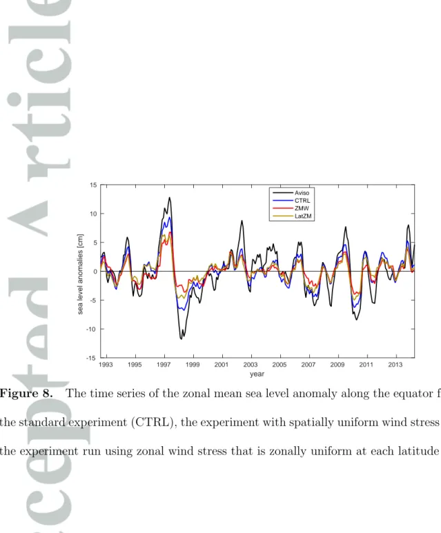
The spatial structure of the wind stress, nevertheless, does matter for the amplitude of the WWV along the equator. This is illustrated in Figure 8 showing the time series of the modelled zonal mean sea level along the equator (corresponding to the WWV) compared to AVISO data. We first note that the amplitude captured by the standard model (labelled CTRL) is generally less than that seen in AVISO, although still a significant fraction of the latter, and that the two time series are highly correlated. Next we note that the amplitude in the model run with spatially uniform forcing (labelled ZMW) is less than that in CTRL indicating a role for the spatial structure of the wind forcing in determining
the amplitude of the WWV. In a further experiment (labelled LatZM) only the zonal wind stress is used and this is given by the time series of the zonal mean of the zonal wind stress at each latitude and so has no variations with longitude. Generally, this increases the amplitude of the WWV along the equator compared to ZMW but still does not explain all the amplitude captured by CTRL, implying a role for zonal variations in the zonal wind stress along the equator for determining the amplitude of the WWV (note that the WWV in CTRL does not depend on the meridional wind stress as can easily be shown by running an experiment driven by the zonal wind stress only).
To understand this further, we note that zonally integrating equation (12) gives us the equation for ¯ηn, the contribution to ¯η from mode n,
(λE−λW)∂η¯n
∂t + Hn acosθ
∂
∂θ
(∫ λE
λW
cosθvndλ
)
= 0. (17)
where λE and λW are the longitudes at the eastern and western boundaries of the model domain, respectively. Clarke[2010] noted that in his analytic solutions, there is a tendency for the zonal and meridional divergence to cancel (as in the Sverdrup balance). However, as is clear from equation (17), for ¯ηnto change, there must be a net meridional divergence at the equator, as indicated by the derivative with respect to latitude. We have seen that to understand the basic dynamics it is enough to consider the case with spatially uniform wind forcing (for which the Sverdrup transport is zero). Consider the spin-up from a state of rest with ηn = 0 following the sudden switch-on of a spatially uniform zonal wind forcing. For eastward wind forcing, the associated Ekman transport leads to convergence on the equator and an increase in ηn, consistent with the picture at zero lag in Figure 7b,c. More than an equatorial Rossby radius from the equator, there is
propagates to the equator as Kelvin waves along the western boundary and then along the equator as equatorial Kelvin waves, leading to the negative correlation in Figure 7b,c at positive lags. It should be noted that the effect of wave propagation is to counter the Ekman convergence/divergence so that in steady state, u = v = 0 and the zonal wind stress is exactly balanced everywhere by the zonal pressure gradient given by an east-west slope in ηn (e.g. McCreary [1981])2. The correlations we see in Figure 7b,c therefore arise from the incomplete nature of the adjustment to the changing wind forcing across the model domain, including the off-equatorial regions, with longer lags the higher the mode, consistent with the longer adjustment time the higher the mode. This interpretation is basically as described in the review paper byNeelin et al.[1998] but here nicely illustrated using our multi-mode model and shown to be consistent with satellite altimeter data, i.e.
AVISO.
4. Summary
We have used a multi-mode shallow water model to examine sea level vari- ability as seen in satellite altimetry (AVISO) over the period 1993-2014 (see http://www.aviso.altimetry.fr/duacs/). The weighting given to each mode was assigned by fitting the model results to the observed sea level variability along the equator. The weighting in turn defines the vertical profile for the wind stress forcing which, as can seen in Figure 1b,c is strongly surface intensified, as one would expect. Using 7 or more modes, it was not possible to assign a realistic weight to each mode, presumably because the signal associated with mode 7 or higher cannot be extracted from the AVISO data.
Since the 6th mode is associated with basically zero amplitude, we used the first 5 modes for our study.
The results show a remarkable agreement between the model sea level and the AVISO data, particularly along the equator but also at higher latitudes where the main events in the monthly mean AVISO data are captured. The model successfully captures the ENSO events of various strengths and flavours, including the conventional El Ni˜no events of 1997/98, 2006/07 and 2009/10) and the Modoki El Ni˜no events of 1994/95, 2002/03 and 2004/05 [Ashok et al., 2007] as well as the 1995/96, 1998/99, 2007/08 and 2010/11 La Ni˜na events. The dominance of the second baroclinic mode is apparent, although with some role for modes 1,3 and 5, particularly in the western equatorial Pacific for mode 1, the eastern equatorial Pacific for mode 5, and both regions for mode 3. The higher modes are particularly prominent during the major El Ni˜no events of 1997/98, 2006/07 and 2009/10 (see Figure 4) when the wind forcing is particularly large in amplitude. We argue that one reason for differences in the weighting assigned to the different modes here from previous studies is the freedom we give the model to choose the vertical profile for the wind forcing in the model based on the fitting to the altimeter data.
An interesting feature of our results is the presence of a pivot point in the western Pacific on the equator, either side of which sea level variations tend to be 180◦ out of phase. The placement of the pivot point seems to depend mostly on the fact that most of the variations in zonal wind stress are found in the western part of the basin, although there is also a signature from the recharge/discharge mechanism in which eastward/westward zonal mean zonal wind stress anomalies are associated with a downward/upward displacement of the zonal mean thermocline along the equator at zero lag. We also showed that the recharge/discharge mechanism in the model does not depend for its basic dynamics on the spatial structure of the wind forcing and, in particular, on the Sverdrup transport
as in the original theory of Jin [1997], and is more in agreement with the approach of Clarke [2010]. The spatial structure of the wind forcing nevertheless has a role to play in determining the amplitude of the “warm water volume” along the equator.
Acknowledgments.
Xiaoting Zhu is grateful for funding from the China Scholarship Council (No.201306330071).This study has also been supported by the Deutsche Forschungs- gemeinschaft as part of the Sonderforschungsbereich 754 “Climate-Biogeochemistry in- teractions in the Tropical Ocean”, through the German Ministry for Education and Research (BMBF) through MiKlip2, subproject 01LP1517D (ATMOS-MODINI) and SACUS (03G0837A), and by the European Union 7th Framework Programme (FP7 2007- 2013) under grant agreement 603521 PREFACE project. We are also grateful to two anonymous reviewers for their helpful comments. The data used in this study can be obtain from Xiaoting Zhu (xzhu@geomar.de) on request.
Notes
1. For this choice of lateral eddy viscosity, the damping time scale for a mode with gravity wave speedc= 1 m s−1 is comparable to that implied by the model ofMcCreary[1981] using vertical mixing. Here we have used the equatorial radius of deformation for the length scale to derive the damping time scale for the lateral mixing. The similarity between the two damping time scales shows that the damping we use here is similar to that implied by the McCreary model.
2. It is worth noting that in the general case, the final steady state is given by the Sverdrup balance everywhere in the domain. Since the Sverdrup balance applies to the steady state, at least in the context of the linear dynamics being considered here, it follows immediately that the recharge/discharge mechanism cannot be associated with Sverdrup balance since the recharge/discharge mechanism is fundamentally unsteady.
References
Ashok, K., S. K. Behera, S. A. Rao, H. Weng, and T. Yamagata (2007), El Nino Modoki and its possible teleconnection, J. Geophys. Res., 112(11), 1–27, doi:
10.1029/2006JC003798.
Berrisford, P., D. Dee, K. Fielding, M. Fuentes, P. Kallberg, S. Kobayashi, and S. Uppala (2009), The ERA-Interim Archive, ERA Rep. Ser.,1(1), 1–16.
Brandt, P., M. Claus, R. J. Greatbatch, R. Kopte, J. M. Toole, W. E. Johns, and C. W.
B¨oning (2016), Annual and semi-annual cycle of equatorial atlantic circulation associ- ated with basin mode resonance, J. Phys. Oceanogr., 46(10), 3011–3029.
Busalacchi, A. J., and M. A. Cane (1985), Hindcasts of sea level variations during the 1982-83 el nino, J. Phys. Oceanogr.,15(2), 213–221.
Busalacchi, A. J., and J. J. O’Brien (1981), Interannual variability of the equatorial Pacific in the 1960’s, J. Geophys. Res., 86(C11), 10,901, doi:10.1029/JC086iC11p10901.
Busalacchi, A. J., K. Takeuchi, and J. J. O’Brien (1983), Interannual variabil- ity of the equatorial Pacific Revisited, J. Geophys. Res., 88(C12), 7551, doi:
10.1029/JC088iC12p07551.
Cane, M. A. (1984), Modeling sea level during el nino, J. Phys. Oceanogr.,14(12), 1864–
1874.
Clarke, A. J. (2010), Analytical Theory for the Quasi-Steady and Low-Frequency Equa- torial Ocean Response to Wind Forcing: The Tilt and Warm Water Volume Modes, J.
Phys. Oceanogr., 40(1), 121–137, doi:10.1175/2009JPO4263.1.
Delcroix, T. (1998), Observed surface oceanic and atmospheric variability in the tropi- cal Pacific at seasonal and ENSO timescales: A tentative overview, J. Geophys. Res.,
103(C9), 18,611–18,633, doi:10.1029/98JC00814.
Dewitte, B., G. Reverdin, and C. Maes (1999), Vertical Structure of an OGCM Simulation of the Equatorial Pacific Ocean in 1985-94, J. Phys. Oceanogr., 29(7), 1542–1570.
Dewitte, B., S.-W. Yeh, and S. Thual (2013), Reinterpreting the thermocline feedback in the western-central equatorial pacific and its relationship with the enso modulation, Clim. Dyn.,41(3-4), 819–830, doi:10.1007/s00382-012-1504-z.
Doi, T., T. Tozuka, and T. Yamagata (2010), Equivalent forcing depth in tropical oceans, Dyn. Atmos. Ocean., 50(3), 415–423, doi:10.1016/j.dynatmoce.2010.03.001.
Ebisuzaki, W. (1997), A method to estimate the statistical significance of a correlation when the data are serially correlated, J. Clim., 10(9), 2147–2153.
Forget, G., and R. M. Ponte (2015), The partition of regional sea level variability, Prog.
Oceanogr.,137, Part, 173 – 195, doi:10.1016/j.pocean.2015.06.002.
Gill, A. E. (1982), Atmosphere-Ocean Dynamics, 662 pp., Academic press, san diego, california.
Gill, A. E., and A. J. Clarke (1974), Wind-induced upwelling , coastal currents and sea- level changes, Deep Sea Res.,21, 325–345.
Jin, F.-F. (1997), An Equatorial Ocean Recharge Paradigm for ENSO. Part I: Conceptual Model, J. Atmos. Sci., 54(7), 811–829.
Locarnini, R. A., A. V. Mishonov, J. I. Antonov, T. P. Boyer, H. E. Garcia, O. K.
Baranova, M. M. Zweng, C. R. Paver, J. R. Reagan, D. R. Johnson, M. Hamilton, and D. Seidov (2013), World Ocean Atlas 2013. Vol. 1: Temperature., S. Levitus, Ed.;
A. Mishonov, Tech. Ed.; NOAA Atlas NESDIS,73(September), 40, doi:10.1182/blood- 2011-06-357442.
McCreary, J. (1981), A linear stratified ocean model of the equatorial undercurrent,Phil.
Trans. Roy. Soc. London A, 298(1444), 603–635.
McPhaden, M., J. Proehl, and L. Rothstein (1986), The interaction of equatorial kelvin waves with realistically sheared zonal currents, J. Phys. Oceanogr., 16(9), 1499–1515.
McPhaden, M. J., and X. Yu (1999), Equatorial waves and the 1997–98 el nino, Geophys.
Res. Lett., 26(19), 2961–2964.
Meinen, C. S., and M. J. McPhaden (2000), Observations of warm water volume changes in the equatorial pacific and their relationship to el ni˜no and la ni˜na, J. Clim., 13(20), 3551–3559.
Meinen, C. S., and M. J. McPhaden (2001), Interannual variability in warm water volume transports in the equatorial pacific during 1993-99*, J. Phys. Oceanogr., 31(5), 1324–
1345.
Moon, B.-K., S.-W. Yeh, B. Dewitte, J.-G. Jhun, I.-S. Kang, and B. P. Kirtman (2004), Vertical structure variability in the equatorial pacific before and after the pacific climate shift of the 1970s, Geophys. Res. Lett., 31(3).
Neelin, J. D., D. S. Battisti, A. C. Hirst, F.-F. Jin, Y. Wakata, T. Yamagata, and S. E. Ze- biak (1998), ENSO theory, J. Geophys. Res.,103(C7), 14,261, doi:10.1029/97JC03424.
Philander, S., and R. Pacanowski (1980), The generation of equatorial currents, J. Geo- phys. Res., 85(C2), 1123–1136.
Philander, S. G. (1989), El Ni˜no, La Ni˜na, and the Southern Oscillation, 662 pp., Aca- demic press, San Diego, California.
Picaut, J., and L. Sombardier (1993), Influence of density stratification and bottom depth on vertical mode structure functions in the tropical Pacific, J. Geophys. Res., 98(C8),
14,727, doi:10.1029/93JC00885.
Trenberth, K. E., G. W. Branstator, D. Karoly, A. Kumar, N. C. Lau, and C. Ropelewski (1998), Progress during TOGA in understanding and modeling global teleconnections associated with tropical sea surface temperatures, J. Geophys. Res., 103(C7), 14,291–
14,324, doi:10.1029/97jc01444.
Yu, X., and M. J. McPhaden (1999), Seasonal variability in the equatorial pacific,J. Phys.
Oceanogr.,29(5), 925–947.
Table 1. Projection coefficients Gn (unit: m1/2) obtained by the fitting when using different numbers of modes
G1 G2 G3 G4 G5 G6 G7 G8 G9
2 modes 7.07 29.73 - - - -
3 modes 7.85 16.01 28.00 - - - -
4 modes 7.96 18.66 10.25 17.73 - - - - -
5 modes 7.76 18.48 14.91 4.25 9.36 - - - -
6 modes 7.76 18.48 14.92 4.15 9.54 -0.13 - - - 7 modes 7.58 18.30 16.45 -1.66 33.98 -49.09 31.41 - - 8 modes 7.54 18.40 16.12 -1.59 36.42 -64.39 62.43 -17.15 - 9 modes 7.71 19.26 13.07 3.79 18.12 4.11 -164.94 317.01 -178.16
Table 2. Projection coefficients Gn (unit: m1/2) when specifying the vertical profile G(z) given by G(z) =HE/D over a surface Ekman layer of depth D and G(z) = 0 below.
D G1 G2 G3 G4 G5 G6 50 m 18.63 19.88 13.24 12.71 13.23 11.81 100 m 18.41 18.39 10.48 7.92 5.90 2.98 150 m 16.54 14.92 6.41 2.51 -0.55 -2.64 200 m 15.34 11.87 2.76 -1.47 -3.66 -3.23 250 m 14.24 9.21 0.08 -3.44 -3.82 -1.31
−0.05 0 0.05 0.1 0
200 400 600 800 1000 1200 1400 1600 1800 2000
3000
4000
5000
depth[m]
(a) pressure vertical structures
1st 2nd 3rd 4th 5th mode
0 1.50
0 200 400 600 800 1000 1200 1400 1600 1800 2000
3000
4000
5000
(b) wind forcing profile based on 5 modes
0 1.50
0 200 400 600 800 1000 1200 1400 1600 1800 2000
3000
4000
5000
(c) wind forcing profile based on 4 or 6 modes
4 6
Figure 1. (a) The vertical structure functions, ˆpn, for modes 1-5. (b) The wind stress profile, G(z), obtained using 5 modes. (c) same as (b) but using 4 (dashed line) and 6 modes (solid line).
(a) zonal wind stress
160°E 120°W 1993
1995 1997 1999 2001 2003 2005 2007 2009 2011 2013
160°E 120°W (b) aviso
160°E 120°W (c) CTRL multi−mode
−0.01 0 0.01 (d) zonal mean of zonal wind stress
160°E 120°W (e) ZMW multi−mode
cm
−8 −6 −4 −2 0 2 4 6 8
−0.06 −0.04 −0.02 0 0.02 0.04 0.06
Nm−2
Figure 2. Hovmoeller diagrams along the equator for (a) the zonal wind stress from ERA- Interim used to drive the standard model and (d) the zonal mean zonal wind stress. Also shown are monthly mean sea level anomalies along the equator for (b) AVISO, (c) the multi-mode model (standard version), (e) the model when driven by the time series of zonal mean zonal wind stress along the equator (shown in (d)) and zero meridional wind stress (experiment ZMW). Units are Nm−2 for wind stress and centimetres for sea level.
10°S
160°E 120°W 1993
1995 1997 1999 2001 2003 2005 2007 2009 2011 2013
(a) 5°S
160°E 120°W
5°N
160°E 120°W
10°N
160°E 120°W
15°N
160°E 120°W cm−8
−6
−4
−2 0 2 4 6 8
10°S
160°E 120°W 1993
1995 1997 1999 2001 2003 2005 2007 2009 2011 2013
(b) 5°S
160°E 120°W
5°N
160°E 120°W
10°N
160°E 120°W
15°N
160°E 120°W cm−8
−6
−4
−2 0 2 4 6 8
Figure 3. Hovmoeller diagrams of sea level anomalies along 10S, 5S, 5N, 10N and 15N from (a) AVISO and (b) the standard version of the multi-mode model. Units are centimeters.
1993 1995 1997 1999 2001 2003 2005 2007 2009 2011 2013
160°E 120°W mode 1
160°E 120°W mode 2
160°E 120°W mode 3
160°E 120°W mode 4
160°E 120°W mode 5
cm−8
−6
−4
−2 0 2 4 6 8
Figure 4. Hovmoeller diagrams along the equator for the contribution to sea level from modes 1-5 in the standard model run. Units are centimeters.
Aviso
150°E 160°W 110°W 10°S
EQ 10°N
(a)
cm0 2 4 6 8
multi−mode model
150°E 160°W 110°W 10°S
EQ 10°N
(b)
cm 0 2 4 6 8
mode 1
150°E 160°W 110°W 10°S
EQ 10°N
(c)
cm0 2 4
mode 2
150°E 160°W 110°W 10°S
EQ 10°N
(d)
cm 0 2 4
mode 3
150°E 160°W 110°W 10°S
EQ 10°N
(e)
cm0 2 4
mode 4
150°E 160°W 110°W 10°S
EQ 10°N
(f)
cm 0 2 4
mode 5
150°E 160°W 110°W 10°S
EQ 10°N
(g)
cm0 2 4
Figure 5. The standard deviations of monthly mean sea level anomalies from (a) AVISO, (b) the multi-mode model and (c-g) the contribution from modes 1-5, respectively. Units are centimeters.
multi−mode model
150°E 160°W 110°W 10°S
EQ 10°N
(a) mode 1
150°E 160°W 110°W
10°S EQ 10°N
(b)
mode 2
150°E 160°W 110°W 10°S
EQ 10°N
(c) mode 3
150°E 160°W 110°W
10°S EQ 10°N
(d)
mode 4
150°E 160°W 110°W 10°S
EQ 10°N
(e) mode 5
150°E 160°W 110°W
10°S EQ 10°N
(f)
−1.0
−0.8
−0.6
−0.4
−0.2 0.0 0.2 0.4 0.6 0.8 1.0
Figure 6. The correlation coefficients between monthly mean sea level anomalies from AVISO and those from (a) the multi-mode model and (b-f) the contribution from modes 1-5, respectively.
lag(months)
0 6 12 18 24 30 36 42 48 54 60 66 72 78 84
-0.4 -0.2 0 0.2 0.4 0.6 0.8
1 (a) autocorrelation of zonal mean zonal wind stress
lag(months)
-24 -22 -20 -18 -16 -14 -12 -10 -8 -6 -4 -2 0 2 4 6 8 10 12 14 16 18 20 22 24 -0.6
-0.4 -0.2 0 0.2 0.4 0.6 0.8 1
wind lags wind leads
(b) lagged correlation between zonal mean sea level and wind stress anomalies
Aviso CTRL ZMW
lag(months)
-24 -22 -20 -18 -16 -14 -12 -10 -8 -6 -4 -2 0 2 4 6 8 10 12 14 16 18 20 22 24 -1
-0.8 -0.6 -0.4 -0.2 0 0.2 0.4 0.6 0.8 1
wind lags wind leads
(c) lagged correlation between zonal mean sea level and wind stress anomalies
1st 2nd 3rd 4th 5th
mode
Figure 7. (a) The autocorrelation of zonal mean zonal wind stress along the equator. (b) Lagged correlations between zonal mean monthly sea level anomalies and zonal mean zonal wind stress anomalies along the equator for AVISO, the multi-mode model in the standard version (labelled CTRL) and model run driven by the time series of zonal mean zonal wind stress along the equator (labelled ZMW). (c) As (b) but for each of modes 1-5 from the standard model run.
The horizontal lines indicate the thresholds for correlations to be different from zero at the 95%
level and are computed using the method ofEbisuzaki [1997].
year
1993 1995 1997 1999 2001 2003 2005 2007 2009 2011 2013
sea level anomalies [cm]
-15 -10 -5 0 5 10 15
Aviso CTRL ZMW LatZM
Figure 8. The time series of the zonal mean sea level anomaly along the equator from AVISO, the standard experiment (CTRL), the experiment with spatially uniform wind stress (ZMW) and the experiment run using zonal wind stress that is zonally uniform at each latitude (LatZM).