Modeling MYC-dependent regulation of gene expression and cell metabolism in B-cell lymphomas
DISSERTATION ZUR ERLANGUNG DES DOKTORGRADES DER NATURWISSENSCHAFTEN (DR. RER. NAT.)
DER FAKULT ¨ AT F ¨ UR BIOLOGIE UND VORKLINISCHE MEDIZIN DER UNIVERSIT ¨ AT REGENSBURG
vorgelegt von
Franziska Taruttis-Glagoleff
aus Eisleben
im Jahr 2020
Der Promotionsgesuch wurde eingereicht am:
08.10.2020
Die Arbeit wurde angeleitet von:
Prof. Dr. Rainer Spang Unterschrift:
Franziska Taruttis-Glagoleff
Declaration of personal contribution to published manuscripts
Parts of the thesis are composed of the following published manuscripts:
• Chapter 2 largely corresponds to the manuscript of Taruttis et al. (2017): I devel- oped the method described together with my co-author Maren Feist. I performed the experimental design, generated the synthetic data and analysed the sequence data. I performed the statistical and bioinformatical analysis and prepared the figures except for Figure 2.1, which was kindly provided by Maren Feist.
Maren Feist (Department of Haematology and Medical Oncology of the University Medical Center G¨ottingen) carried out all wet lab experiments. RNA-seq was done by Dr. Gabriela Salinas-Riester (Head of Core Microarray and Deep-Sequencing Core Facility, University Medical Center G¨ottingen)
• Chapter 3 largely corresponds to the manuscript of Taruttis et al. (2015): I devel- oped the computational method described. I performed the experimental design and generated the synthetic data sets. I performed the statistical and bioinformat- ical analysis and prepared all presented figures.
Acknowledgement
Throughout working at my thesis at the Department of Statistical Bioinformatics at the Institute of Functional Genomics (University of Regensburg) I have received a great deal of support and assistance. The work was supported by the BMBF grant e:Bio:MMML- MYC-SYS and the Bavarian Genome Network BayGene.
I am very grateful to my supervisors Julia C. Engelmann and Rainer Spang for suggesting the topic, for their support and advice during the entire doctorate, for pushing me to sharpen my thinking and to write this thesis under their guidance. Especially, I am thankful to Rainer Spang for providing a friendly, motivating and inspiring place at the Department of Statistical Bioinformatics.
I would like to acknowledge my mentoring team, Tobias M¨uller and Wolfram Gronwald, for fruitful discussions and their helpful advice.
This work would not have been possible without collaboration. Thus, I want to thank Maren Feist and Dieter Kube, Philipp Schwarzfischer, Wolfram Gronwald and Katja Dettmer-Wilde and Karsten Kleo, Lora Dimitrova and Michael Hummel.
I want to thank Julia C. Engelmann and Katharina Hirsch for proofreading this thesis.
Your advice brought my work to a higher level.
Many thanks to our secretaries Eva Engel and Sharon Petersen, who were always ready to lend an ear and for their help with both minor and major problems. I also want to thank Kinga Ay from the Regensburg International Graduate School of Life Sciences for her support during thesis submission.
During the time I worked on this thesis, I enjoyed fruitful discussions, about our work and about everything else with the whole group and the alumni of the Department of Statistical Bioinformatics. Special thanks got to Katharina Hirsch, Claudio Lottaz, Martin Pirkl, Anton Moll, Christian Hundsrucker, Chistian Kohler, Thorsten Rehberg and Paula Perez-Rubio.
Furthermore, I like to thank the ”lunch club” of the Institute of Functional Genomics for encouraging me whenever it was needed. In particular, I would like to mention Nadine Aßmann, Claudia Samol, Nadine N¨urnberger, Elke Perthen, Katja Dettmer-Wilde and Wolfram Gronwald.
Last but not least, I would like to thank my whole family for their continuing support.
Especially, I am grateful to my husband Nico and my beloved children Kuno and Klara.
I could not have completed this dissertation without their patience, their understanding and their constant encouragement.
Summary
The oncogene MYC plays an important role in B cell lymphoma pathogenesis. Despite more than 30 years of MYC research there are still open questions concerning its func- tion and how to target MYC in lymphomagenesis. Thus, this work aims to examine the causal relationships between MYC and the transcriptome and metabolome in a B cell lymphoma cell line by computational methods. The data set covers RNA-seq and mass spectrometry measurements of the same cell line. The underlying data is purely observational, no intervention is needed since causal inference techniques enable virtual experiments in theory. The first part of this thesis addresses three issues:
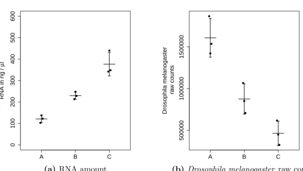
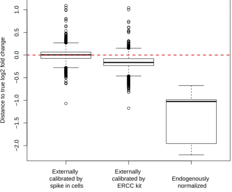
First, the analysis of the RNA-seq data from cells with overexpressedMYC is challenging since MYC is a transcriptional amplifier. There is no de novo activation of genes by the elevated MYC, but an amplification of all presently expressed genes. This behavior is accompanied with an increase in cell size and an increase of RNA amount. Thus, the comparison of lymphoma cells with a highMYC expression with normal B cells by RNA- seq standard pipelines is difficult, since current normalization methods require a constant RNA amount across samples. I present a method that usesDrosophila melanogaster cells as a spike-in to calibrate the data to the number of cells in the sample (Taruttis et al., 2017). I demonstrate that, in case of transcriptional amplification in the B cell lymphoma cell line the use of an external spike-in is mandatory to observe the global gene expression changes. Furthermore, the Drosophila melanogaster spike-in normalization outperforms other calibration methods, including the use of the commercially available ERCC spike- ins.
Second, Maathuis et al. (2010) presented the first high throughput analysis of virtual intervention experiments. Their ground-breaking IDA method (Maathuis et al., 2009) will have a lasting effect on the field of systems biology. Further developments of the IDA method recommended a subsampling strategy for the estimation of causal effects from observational data (Stekhoven et al., 2012). I extend IDA and its extension CStaR by an- alyzing the distribution of causal effects and call the method Accumulation IDA (aIDA) (Taruttis et al., 2015). aIDA improves the prediction of causal effects in comparison to Maathuis et al. (2009) and (Stekhoven et al., 2012).
Third, causal structure learning by the PC algorithm (Spirtes and Glymour, 1991; Kalisch and B¨uhlmann, 2007), the first step of both IDA and aIDA, assumes that the underlying structure is sparse. However, the application of the spike-in methods to B cell lymphoma data sets with MYC overexpression results in highly correlated data. Thus, the under- lying causal structure is very likely not sparse. I assume that this is a consequence of the global role of Myc in gene expression (Lin et al., 2012; Nie et al., 2012). Thus, we
observe no technical artifact but a real biological process. I show that using the MMHC algorithm instead of the PC algorithm together with my accumulation method outper- forms aIDA for highly correlated datasets. However, the MMHC-aIDA method breaks down, too, when the density of the underlying causal structure becomes too high.
The second part of the thesis presents a causal inference analysis of a B cell lymphoma cell line. We decided for the P493-6 cell line due to its doxycycline-dependant promoter to switch MYC on or off, which allows for an examination of the causal relationships of MYC under the same epigenetic conditions. RNA-seq and mass spectrometry data are measurements of the transcriptome and the metabolome of the cell line and are the input of the causal inference analysis. I show that the selection of the method to estimate the causal effects highly depends on the data structure. While the highly correlated RNA- seq dataset shows the best results with the MMHC-aIDA method, the mass spectrometry data performs well with aIDA. The analysis of RNA-seq data shows that MYC upregu- lates the majority of genes in the dataset. MYC further shows a positive causal effect on the majority of the metabolites. These findings are in line with the hypothesis thatMYC is a trancriptional amplifier. Some of the causal effects of MYC on the transcriptome and metabolome are already known, others can be high priority candidates for future wet lab experiments.
Contents
1 Introduction 1
1.1 The oncogene MYC and its role in B cell lymphoma pathogenesis . . . . 1 1.1.1 B cell lymphoma - a very heterogeneous group of cancer . . . 1 1.1.2 The MYC oncogene is a hallmark of B cell lymphoma pathogenesis 5 1.1.3 MYC - a transcriptional amplifier and resulting consequences for
data normalization . . . 10 1.2 On the estimation of causal effects from observational data . . . 12 1.2.1 Correlation does not imply causation . . . 12 1.2.2 Estimation of causal effects from observational data when the causal
structure is known . . . 15 1.2.3 Causal structure learning . . . 19 1.2.4 Estimation of causal effects from observational data with unknown
causal structure . . . 22 1.3 Outline . . . 22
I Methods 26
2 External calibration with Drosophila whole-cell spike-ins delivers abso- lute mRNA fold changes from human RNA-Seq data 27 2.1 Section introduction: Global changes of RNA amount between conditions
require special normalization techniques . . . 27 2.2 Sample preparation and data analysis . . . 29 2.2.1 Experimental design . . . 29
2.2.2 Preparation of a custom genome . . . 31
2.2.3 Normalization and differential gene expression analysis . . . 31
2.3 Results . . . 32
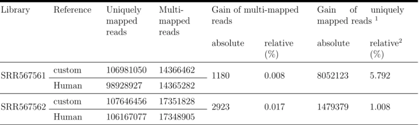
2.3.1 Drosophila melanogaster cells are suitable spike-in cells for human RNA-seq studies . . . 32
2.3.2 The calibration by whole cell spike-ins can be done in multiple ways 34 2.3.3 Spike-in adjusted data provides estimates of differential expression that are calibrated to the total number of cells . . . 34
2.3.4 Whole cell spike-in calibration outperforms other calibration methods 38 2.3.5 Whole cell spike-in calibration affirms MYC driven general tran- scriptional amplification in human P493-6 B-cells . . . 38
2.3.6 General transcriptional amplification in B cells is not limited to MYC regulation . . . 41
2.4 Discussion and conclusions . . . 41
3 aIDA - A statistical approach to virtual cellular experiments 44 3.1 Motivation . . . 44
3.2 The aIDA algorithm . . . 50
3.3 Results . . . 51
3.3.1 Parameter calibration . . . 51
3.3.2 Performance on simulated datasets . . . 52
3.3.3 Application to gene expression data of S.cerevisiae deletion strains 55 3.4 Discussion and conclusions . . . 57
4 Estimation of causal effects from highly correlated data 59 4.1 Motivation . . . 59
4.2 MMHC-aIDA algorithm . . . 62
4.3 Results . . . 63
4.3.1 Performance on simulated datasets . . . 63
4.4 Discussion . . . 63
II Causal analysis of MYC -dependent gene expression and cell metabolism of a B cell lymphoma cell line 67
5 Experimental setup and data preparation 68 5.1 Experimental setup . . . 685.2 Data normalization . . . 70
5.2.1 Gene expression data . . . 70
5.2.2 Metabolomics data . . . 71
6 Causal inference analysis 75 6.1 The Estimation of causal structures depends on the correlation pattern of the samples . . . 75
6.1.1 Gene expression data . . . 75
6.1.2 Metabolomics data . . . 75
6.2 Causal relationships between the transcriptome andMYC . . . 78
6.3 Causal relationships between the metabolome andMYC . . . 83
6.4 Discussion . . . 86
III Discussion and Outlook 90 IV Appendix 100
A Experimental setup of RNA-seq experiment 101 A.1 Cell culture and cell spike-in . . . 101A.2 RNA Isolation and ERCC spike-in . . . 102
A.3 RT-qPCR . . . 102
A.4 RNA sequencing . . . 103
B Experimental setup of metabolomics experiment 104 B.1 Cell culture and extraction of cell pellets and supernatants . . . 104
B.2 Mass spectrometry . . . 104
C Data generation and preprocessing 105 C.1 Simulation of artificial datasets . . . 105
C.2 Hughes et al. (2000) dataset . . . 106
C.3 Lenstra et al. (2011) dataset . . . 106
D Definition of the target set of causal effects 107 D.1 Hughes and Holstege data . . . 107
D.2 Artificial datasets . . . 107
E CStaR parameters 109
CHAPTER 1
Introduction
1.1 The oncogene MYC and its role in B cell lym- phoma pathogenesis
1.1.1 B cell lymphoma - a very heterogeneous group of cancer
Cancer is a disease characterized by abnormal cell growth and the ability to spread (metastasis) or to invade other neighboring tissues, which may occur in every tissue of the body. The World Cancer Report documents approximately 18.1 million new cases and 9.6 million cancer related deaths in 2018 (Wild et al., 2020). Moreover, the World Health Organization (WHO) assumes that the number of new cases increases by approximately 50 % within the next 20 years. From a genetic point of view cancer is caused by genomic alterations. Lengauer et al. (1998) organizes the various amount of these alterations into four groups: (i) the insertion or deletion of only a small number of nucleotides, (ii) a gene amplification (increase of the number of copies of a gene), (iii) the chromosomal translocation, which is a rearrangement of parts of two different chromosomes and (iv) an alteration of chromosome number by gain or loss of whole chromosomes (aneuploidy).
There are more than 100 different types of cancer due to the high number of different tissues that might be affected and the complexity of genetic arrangement. Ciriello et al.
(2013) summarizes the analysis of genomic alterations in the following two statements: (i) tumors occurring in the same tissue can be highly diverse with respect to their genomic profile (Network et al., 2012), (ii) whereas tumors from very different tissues can show similar genetic patterns (Verhaak et al., 2010). Hanahan and Weinberg (2011) reduced
the complexity of cancer to eight hallmarks, which provide a logical framework how cancer emerges and develops:
1. Cancer cells stimulate their own growth.
2. Cancer cells disturb or switch off programs in the cell, that control proliferation.
3. Cancer cells avoid apoptosis.
4. Cancer cells have unlimited replicative potential.
5. Tumors require the induction of angiogenesis.
6. Cancer cells are able to invade neighboring tissues and to metastasize.
7. Cancer cells undergo a reprogramming of cellular energy metabolism.
8. Cancer cells defend themselves against attack by immune cells.
Lymphoma is a group of cancer, which affects the human cells that defend the body against pathogens and infected cells, the lymphocytes. In 2018, 589.580 new cases of lym- phoma and about 274.891 lymphoma related deaths have been reported worldwide (Bray et al., 2018). There are two groups: Hodgkin and Non-Hodgkin Lymphoma. Hodgkin Lymphoma are characterized by the existence of Reed-Sternberg cells, a distinctive cell type used for diagnostic purposes. While the five year survival rate of Hodgkin lym- phoma is about 90 %, the survival rate of Non-Hodgkin Lymphoma highly depends on the subtype. There are more than 60 different subtypes of Non-Hodgkin Lymphoma.
About 90 % of Non-Hodgkin Lymphomas originate from a B cell, a type of white blood cells, that plays a central role in the adaptive immune system. This specific immune response eradicates invading pathogens, called antigens, without damaging any endoge- nous molecules. These antigens are bound by the B cell receptor (BCR), which B cells express on their cell membrane. A BCR consists of two heavy (H) polypeptide chains and two light (L) polypeptide chains of immunoglobulines (Ig) covalently connected by a disulfit bridge and CD79A and CD79B molecules, that transmit signals after BCR cross linking (K¨uppers et al., 1999a). Each B cell produces exactly one highly specific kind of immunoglobulines. Specific genetic processes during B cell development, that allow the H and L chains for rearrangement and point mutations enable the B cells to build a wide variety of more than 1012 different antibodies (M˚artensson et al., 2010). However, while these mechanisms are responsible for the high flexibility and specificity of the human adaptive immune response, they also carry a great danger. The need of these genetic re- arrangements includes the high potential to end up in unwanted genetic alterations and
with that may trigger lymphomagenesis (Basso and Dalla-Favera, 2015). Chromosomal translocations, which do often involve an Ig gene and an oncogene, are a hallmark of B cell lymphoma pathogenesis (K¨uppers and Dalla-Favera, 2001; Willis and Dyer, 2000).
The oncogene comes under the control of an Ig promoter, which leads to an uncontrolled upregulation of the oncogene and with that triggers lymphoma pathogenesis. When a lymphoma is developed at a certain state of the B cell development process, the genetic state of the cell of origin is ”frozen” and this maturation state defines the lymphoma subtype (K¨uppers et al., 1999b; Shaffer et al., 2002).
Thus, to understand the huge diversity of B cell lymphomas we need to get insights into the B cell developmental process.
How does a B cell develop, which processes cause the genetic and functional diversity of the antibodies and how do errors within these processes lead to lymphoma? There are three specific breakpoints of chromosomal translocations which can be assigned to three different stages of the developmental process (K¨uppers, 2005;
Robbiani and Nussenzweig, 2013):
(i) V(D)J recombination The B cell development starts in the bone marrow, where a lymphoid progenitor cell evolves into a pre B cell that expresses a pre-BCR.
This pre-BCR consists of two Ig heavy (H) and surrogate light (SL) polypeptide chains.
The H and L chains consist of variable (V) and constant (C) regions. According to their constant region the heavy chains are divided into five classes: the α, δ, , γ and µ chains.
And depending on that grouping the antibodies are classified as IgA, IgD, IgE, IgG and IgM. The variable regions are completed by a Joining (J) and Diversity (D) region.
To build a functional antibody, the pre-BCR undergoes a process called V(D)J recom- bination of the µ-chains which rearranges these V, J and D gene segments. This rear- rangement enables the B cells to produce very diverse antibodies, which are important for the adaptive immune response to new pathogens. Even if this process is well controlled by different mechanisms (Jung et al., 2006), errors during V(D)J recombination pro- cess can drive lymphomagenesis by introducing unwanted chromosomal translocations.
A well-examined example is the BCL2-IgH translocation in follicular lymphoma. The BCL2 gene is located on chromosome 18 and encodes for the BCL2 family of regulatory proteins (Adams and Cory, 2007). The translocation brings the BCL2 gene under the control of a Ig heavy chain promotor (J¨ager et al., 2000; Tsujimoto et al., 1985, 1988).
This leads to a dramatically increase of BCL2 expression and an increased BCL2 expres- sion increases the probability of a cell to avoid apoptosis (Cleary et al., 1986; Tsujimoto
et al., 1984), which is a hallmark of carcinogenesis (Hanahan and Weinberg, 2011).
(ii) Somatic hypermutation After V(D)J recombination the surrogate L chains are replaced by corresponding valid L chains to form a IgM antibody. Thus, the IgM antibody is the first antibody which is produced during B cell development. The affinity of these IgM antibodies to bind their corresponding antigen is still low in comparison to the other classes. To account for that, this class of antibodies is able to form pentamers when it is secreted and with that the antigen is tackled by 10 antigen binding sites.
If this pre-BCR is functional and non-autoreactive, the immature naive B cell leaves the bone marrow, starts to express IgD antibodies on its membrane and moves to the secondary lymphoid organs, for example the spleen, the lymph nodes or the tonsils.
Immature B cells which do not pass this checkpoint undergo apoptosis (Rajewsky, 1996).
After activation by an antigen and mediated by T cells the naive B cells proliferate intensively and form the germinal center. During its maturatin the germinal centers form two separate compartments: the dark zone and the light zone. In the dark zoe of the germinal centers the B cells undergo a process to remodel their immunglobulin genes and to express high-affinity antibodies: the somatic hypermutation. The B cells are extremely proliferative and undergo point mutations, gene amplifications and deletions in the V regions of the BCR. This ensures a huge variety of different antibodies with different affinity to the antigen. However, Pasqualucci et al. (2001) demonstrated, that hypermutated regions of some protooncogenes are prone to chromosomal translocations in Diffuse Large B Cell Lymphomas (DLBCLs). Thus, errors during somatic hypermutation may introduce unwanted chromosomal translocations.
(iii) Class switch recombination The B cells with the BCR altered by somatic hypermutation leave the dark zone of the germinal centers and enter the light zone.
Here the cells are selected by T helper cells and follicular dendritic cells for an improved antigen binding. B cells which do not improve their affinity to the antigen by somatic hypermutation undergo apoptosis. Some B cells reenter the dark zone to further improve their affinity (De Silva and Klein, 2015). Before they leave the light zone these B cells can do a class switch recombination, where the Ig gene of the constant region is changed to build IgG, IgE and IgA antibodies. This results in the same antigen-binding domain, but a different class of antibodies (K¨uppers, 2005). The five different classes of antibodies can attack the antigens in different ways. They occur in different proportions and the IgG is the largest group of antibodies. However, class switch recombination is the third process which may generate chromosomal translocations. A well-described example is the t(8;14) mutation, which brings the MYC oncogene under the control of an Ig gene.
This translocation is a primary event during sporadic Burkitt’s lymphoma pathogenesis (Taub et al., 1982; Janz et al., 2003; K¨uppers and Dalla-Favera, 2001; Dalla-Favera et al., 1983; Ramiro et al., 2006). Finally, the high-affinity B cells mature to effector B cells, which secrete huge amounts of antibodies to neutralize and destroy antigens and memory B cells, that trigger a more effective immune response in case of re-infection with the antigen.
Beyond the chromosomal translocations mentioned before, there are many other different kinds of mutations, like deletions, insertions or other genetic alterations that may trigger lymphomagenesis (Seifert et al., 2013). Each subtype of B cell lymphoma can be assigned to a specific maturation state based on mutations in the Ig V region and gene expression profiling. This assigned maturation state is termed the ”cell of origin”
(Shaffer III et al., 2012). For example, Burkitt’s lymphoma share a similar genetic profile with the B cells in the dark zone of the germinal centers, while the DLBCLs share similarities with the GC light zone B cells (K¨uppers, 2005). However, Shaffer III et al.
(2012) criticize the term ”cell of origin”, since pathogenesis may also start at an earlier state of the maturation process. Thus, after the initial oncogenic event the maturation of the B cell continues until secondary oncogenic hits determine the lymphoma subtype (Shaffer III et al., 2012).
1.1.2 The MYC oncogene is a hallmark of B cell lymphoma pathogenesis
MYC is located on chromosome 8 and plays a central role in B cell lymphomagenesis.
It encodes for transcription factor C-MYC and influences metabolism, proliferation and cell differentiation. Together with MAX, MYC builds a complex, which binds DNA at the E-box promotor region (Kretzner et al., 1992; Amati et al., 1993). MYC’s oncogenic potential appears, when it comes under the control of an Ig gene by chromosomal translo- cation. The resulting upregulation of MYC can induce aggressive B cell lymphomas (Dalla-Favera et al., 1982; Persson and Leder, 1984; Adams et al., 1985). Upregulated MYC is detectable in 30% to 40% of DLBCLs and 70% to 100% of Burkitt lymphomas (Sesques and Johnson, 2017; Johnson et al., 2012; Chisholm et al., 2015; Agarwal et al., 2015; Perry et al., 2013). MYC plays an important role in every hallmark of B cell lymphoma pathogenesis, which is underpinned by the following examples:
(i) Cancer cells stimulate their own growth. Even if proliferative signaling in cancer cells is well understood, many details especially with respect to therapeutic ap- proaches requires further research. Hanahan and Weinberg (2011) present three ways how
cancer cells maintain the proliferative signaling. First, they produce ligands for growth factors themselves. Second they send signals to normal cells in their environment, which causes these normal cells to produce growth factors for the cancer cells. And third, they increase the amount of growth factor receptors on their surface to become hyperrespon- sive (Hanahan and Weinberg, 2011).
A major growth factor signaling pathway in humans is the PI3K-AKT-mTOR path- way and the deregulation of this pathway may lead to cancer. In a nutshell, activated Phosphoinositid-3-Kinase (PI3K) causes cell growth via Proteinkinase B (AKT), increases metabolic activity and promotes survival (Cantley, 2002). The mechanistic Target of Ra- pamycin (MTOR), a downstream effector of AKT consists of two different complexes.
The mTOR complex 1 (MTORC1) plays a major role in cell growth (Ma and Blenis, 2009) and the mTOR complex 2 (MTORC2) inhibits a MTORC1 repressor, the tuberous sclerosis complex 2 (TSC2) via AKT. MTOR directly activates protein synthesis, lipid synthesis and ribosomal biogenesis (Efeyan et al., 2012).
Deregulated MYC in Burkitt’s lymphoma increases the expression of MIR17HG a precur- sor RNA for the micro-RNA miR-19 (Olive et al., 2009; Xiao et al., 2008). miR-19 is an inhibitor of Phosphatase and Tensin homolog (PTEN), a well-known tumor suppressor gene which downregulates PI3K. Thus, the inhibition of PTEN increases the expression of PI3K, which drives the survival of Burkitt’s lymphoma cells (Schmitz et al., 2012).
(ii) Cancer cells disturb or switch off programs in the cell that control pro- liferation. Differentiated, mature cells have programs to inhibit cell growth and pro- liferation. A lot of these programs involve tumor suppressor genes. A typical tumor suppressor gene is the TP53 gene which is regulated by MDM2. During homeostasis, without stress exposure MDM2 ubiquitinates and with that downregulates TP53. Af- ter stress exposure, for example by oxidative stress or DNA damage, TP53 is activated.
When a cell is damaged TP53 triggers cell cycle arrest and, in case of irreparable cell damage, activates apoptosis. In spite of the huge efforts during the past three decades the detailed regulation mechanism is still unknown (Aubrey et al., 2016). MYC has a contradictory function. On the one handMYC increases proliferation, while on the other hand MYC also drives apoptosis via TP53 (Hermeking et al., 1994). This process acts as a failsafe programm to circumvent uncontrolled proliferation. However, in lymphoma cells this second function is most often inactive. For example, about 30%-60% of Burkitt’s lymphoma carry a TP53 mutation (Gaidano et al., 1991; Newcomb, 1995; Preudhomme et al., 1995). In transgenic mice with a translocation similar to the translocation in the majority of Burkitt’s lymphoma, Schmitt et al. (2002) observed that these phenotypes are chemoresistant and develop fast to the terminal stage. In summary, the loss of TP53
and the activation of MYC are an example for mutations that cooperate to increase proliferation and survival.
(iii) Cancer cells avoid apoptosis. Normal cells share the ability to induce a pro- grammed cell death to preserve the homeostatic balance of their tissues. Whenever a cell is damaged and not able to fulfill its normal tasks anymore the program is activated, too.
BCL2 plays an important role in the regulation of programmed cell death, since it consists of pro- and antiapoptotic units and primarily promotes cell survival (Vaux et al., 1988).
Usually, in absence of BCL2, MYC induces apoptosis via BIM (encoded by BCL2L11).
However, in more than 50% of DLBCLsBCL2 is upregulated and inhibitsMYC mediated apoptosis with no effect on the proliferative function (Hoffman and Liebermann, 1998).
Moreover BCL2 mediates chemoresistance (Schmitt and Lowe, 2001). While Reed et al.
(1988) demonstrated the oncogenic potential ofBCL2, additional genomic alterations are needed to develop an aggressive lymphoma and a chromosomal translocation of MYC could take on this role (McDonnell et al., 1989). Neither a mutation ofMYC nor a mu- tation of BCL2 alone causes aggressive lymphomas. However, the combination ofBCL2 mediated survival signals and proliferation signals provided by MYC, also known as a type of Double-hit lymphomas results in low survival rates and a bad prognosis (Johnson et al., 2009).
(iv) Cancer cells have unlimited replicative potential. The ends of the chromo- somes consist of a special DNA structure, called telomers, which prevent the chromosome ends from DNA damage (Muller, 1938; McClintock, 1941). The length of the telomers is related to the life span of the cell since they shorten with increasing age (Harley et al., 1990). Further telomere shortening directly causes cells to pass into a state called senescence (Nelson and Kastan, 1994; Vaziri et al., 1997), characterized by viable cells which cannot divide anymore (Sedivy, 1998). The enzyme complex telomerase which adds telomeric repeats to the chromosome ends (Greider and Blackburn, 1987), hampers this process. Kim et al. (1994) summarize that telomerase is not present in the majority of normal mortal cell cultures, whereas it is present in the majority of immortal and cancer cells. 85 % of human cancers upregulate telomerase to maintain their telomere length and with that avoid to pass to senescence and crisis, while the remaining cancer types use other processes to avoid telomere shortening (Cesare and Reddel, 2010). The telomerase enzyme complex consists of the RNA part called telomerase RNA component (TERC) and the catalytic subunit telomerase reverse transcriptase (TERT). Different studies suggest that MYC acitvates TERT directly (Greenberg et al., 1999; Wang et al., 1998; Wu et al., 1999). Thus,MYC has a direct influence on keeping limitless replicative
potential. Further, inversely Koh et al. (2015) found, that high levels of TERT positively influence MYC stability and with that regulate lymphomagenesis.
(v) Malignant tumors induce angiogenesis Angiogenesis is the ability to form new blood vessels from preexisting ones. This property is essential for the survival of the tumors, since they have to ensure supply of oxygen and nutritients and they have to maintain the possibility to get rid of carbon dioxide and metabolic waste (Hanahan and Weinberg, 2011). MYC triggers the expression of the proangiogenetic factor VEGF and represses thrombospondin, an antiangiogenetic factor (Baudino et al., 2002). Further in lymphoma that carry a translocation betweenMYC and an Ig gene (MYC positive), the repression of MYC puts a stop to angiogenesis and thrombospondin expression which is essential for tumor regression. Thus, MYC induces angiogenesis in lymphoma and plays an important role in tumor maintenance (von Eyss and Eilers, 2011).
(vi) Cancer cells are able to invade neighboring tissues and to metastasize Cancer cells may on the one hand penetrate adjacent tissues, but, on the other hand, spread to organs different and distant from the primary tumor and form secondary tu- mors, which is known as metastasis. The ability of cancer cells to invade neighboring tissues and to metastasize causes approximately 90% of cancer related deaths (Canel et al., 2013; Li and Li, 2014; Mehlen and Puisieux, 2006). Metastatic spread is a complex molecular process known as the invasion-metastasis cascade (Fidler, 2003; Gupta and Massagu´e, 2006; Talmadge and Fidler, 2010). Following Leber and Efferth (2009) the five steps of this cascade include: (i) invasion and migration of individual cells from the primary tumor to neighboring, healthy tissues, (ii) the invasion of blood and lymphatic vessels by the cancer cells, (iii) the circulation of cancer cells via the blood and the abil- ity of these specialized, aggressive cells to tolerate the high concentration of oxygen and cancer-cell-toxic lymphocytes, (iv) the potential of the cancer cells to leave the blood stream again, and (v) the colonization of distant organs together with proliferation and angiogenesis. E-cadherin, encoded by CDH1 (Huntsman and Caldas, 1998), mediates cell-cell adhesions and the loss of E-cadherin is associated with increased cell motility, tumor progression and metastasis (Birchmeier and Behrens, 1994; Canel et al., 2013). Ma et al. (2010) have shown that MYC directly activatesMIR-9, a miRNA, which represses the expression of E-cadherin. These findings suggest that MYC also influences invasion and metastasis. Roehle et al. (2008) found that MIR-9 is upregulated in follicular lym- phoma. Further, Di Lisio et al. (2012) found an upregulation of MIR-9 in DLBCLs and Marginal zone B cell lymphoma and Szenthe et al. (2013) point out, thatMYC activates miR-9 and miR-9 targets E-cadherin. These findings highlight the importance of miR-9
for lymphomagenesis.
(vii) Cancer cells undergo a reprogramming of cellular energy metabolism Normal healthy mammalian cells primarily convert glucose to pyruvat via glycolysis in the presence of free oxygen to generate energy. Pyruvat is further processed to acetyl- CoA, a key molecule in protein and lipid metabolism, by oxidation in the mitochondria (Oxidative phosphorylation). In contrast, if oxygen is absent, normal cells transform pyruvat to lactate (anaerobic glycolysis). Both metabolic pathways produce adenosine triphospahte (ATP), a molecule used for intracellular energy transfer. However, while oxidative phosphorylation produces 36 mol ATP per mol Glucose, the anaerobic glycolysis supplies 2 mol ATP per mol Glucose. Warburg (1956) observed that cancer cells, even under aerobic conditions, increase lactate production. This process is known as Warburg effect or aerobic glycolysis. The benefits of the Warburg effect for the cancer cells and whether its a cause or a consequence of cancer development is not fully resolved, yet (Liberti and Locasale, 2016; Devic, 2016). However, the findings of Le et al. (2012) suggest that the overexpression of MYC increases the glycolytic flux in MYC-driven Burkitt lymphoma. Beyond these findings MYC also influences glutamine metabolism, fatty acid and cholesterol metabolism and regulates ribosome biogenesis, protein and nucleotide biosynthesis (Hsieh et al., 2015). Thus, MYC is a key manipulator of cellular energy metabolism.
(viii) Cancer cells defend themselves against attack by immune cells The immune system prevents cancer development at three levels: (i) it impedes the outbreak of viral infections and with that lowers the probability for virus-induced cancer development, (ii) it neutralizes pathogens fast and prevents chronic inflammation, which might lead to DNA damage increasing the risk to develop cancer, and (iii) cells of the immune system are able to detect cancer cells and to remove them (Swann and Smyth, 2007). Recently, Casey et al. (2016) showed that MYC hampers this detection of tumor cells by inducing the expression of CD47 and PD-L1. While PD-L1 sends a ”‘don’t find me”’ signal mainly induced by IFN-γ, a pro-inflammatory molecule (Casey et al., 2016; He et al., 2015), CD47 sends a ”‘don’t eat me”’-signal to macrophages and dendritic cells (Casey et al., 2016; Spranger et al., 2016). Thus, MYC influences both, the adaptive immune system via PD-L1 and the innate immune system via CD47.
These are just a few examples for the various functions ofMYC during tumorigenesis.
MYC is deregulated in many different ways. In addition to gross genetic events like insertional mutagenesis, amplification and chromosomal translocation (Meyer and Penn,
2008),MYC is also activated by many signaling pathways, e.g. BCR- or NFκB-signaling, without structurally affecting the location of theMYC gene (Sesques and Johnson, 2017).
A deregulation of MYC can be a primary event for example in Burkitt’s lymphoma or a secondary event for example in MYC positive DLBCLs, which is often associated with a poor prognosis (Johnson et al., 2009). However, deregulated MYC alone is not sufficient for lymphomagenesis (Sander et al., 2012). Although upregulatedMYC induces proliferation in BL,MYC also triggers apoptosis by the activation of the p53 pathway and by upregulating the proapoptotic geneBIM (Evan et al., 1992; Hoffman and Liebermann, 2008; Jacobs et al., 1999; Schmitt et al., 1999). More than inducing lymphomagenesis, MYC cooperates with other mutations, as described above. But, the suppression of MYC can reverse lymphomagenesis (Marinkovic et al., 2004). However this reversion does not work in every context. Gabay et al. (2014) summarizes that for example a knock out ofTP53 expression (Giuriato et al., 2006) or a RAS activation (D’Cruz et al., 2001) hampers the reversion of tumorgenesis. Thus, the physiological state of the cell influences the response of the cells to MYC upregulation (Gabay et al., 2014).
1.1.3 MYC - a transcriptional amplifier and resulting conse- quences for data normalization
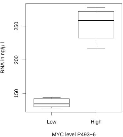
The work of Lin et al. (2012) and Nie et al. (2012) suggests thatMYC is a transcriptional amplifier since they found that MYC leads to the induction of virtually all transcribed genes by a factor of two to three, accompanied with an increase in cell size. Roughly spoken, there is no de novo activation of genes by MYC, since MYC just amplifies the expression of the presently expressed genes depending on the epigenetic background. This behaviour directly influences the RNA amount in a cell. We can observe a much higher amount of RNA in cells with deregulated MYC expression (Figure 1.1). Thus, the RNA amount between cells with deregulated MYC and normal cells differs dramatically. This observation is crucial for data normalization (Lov´en et al., 2012), since current normal- ization methods require the total amount of RNA between different conditions to be constant (see (Li et al., 2017) for a summary of current normalization methods).
These normalization methods are based on the assumption that only a small number of genes change their expression values, while the majority of genes stays constant. Thus, the global upregulation of the majority of presently expressed genes induced byMYC is a violation of this main assumption.
The effect of amplification on data normalization cannot be solved by a computational method alone, since the crucial step happens in the wet lab. Whenever a fixed amount of RNA is taken from our sample for further analysis, the information about the total
Low High
150200250
MYC level P493−6
RNA in ng/µ l
Figure 1.1: RNA concentration of P493-6 cells for two levels of MYC. The P493-6 cell line allows for the induction of MYC via a doxycycline depended promoter to switch MYC on or off. ”‘Low”’ indicates the cells in the presence of doxycycline and represents a low level ofMYC expression, while ”‘High”’ indicates the cells in absence of doxycycline and a high expression level of MYC. The induction of MYC in one million P493-6 cells leads to an increase of the RNA amount per cell(n=10).
amount of RNA per cell is lost. We cannot decide whether there was a real increase of the amount of RNA between two conditions or we just observe technical differences in processing the samples, where we could simply account for. A solution is to measure the amount of RNA before taking a fixed-sized aliquot from the probe (Aanes et al., 2014). However this method is very inaccurate due to the different proportions of differ- ent specimen of RNA within a sample. Moreover, there is a large spread in measurements between different measurement set-ups, e.g. different methods, different technical equip- ment, but also different operator time and skills (Aranda et al., 2009). By adding an external standard to the sample, we can overcome this problem. Lov´en et al. (2012) used the commercially available External RNA control consortium (ERCC) spike in kit, which consists of 92 poly-adenylated transcripts derived fromBacillus subtilis with lengths be- tween 250 and 2000 nucleotides. Adding a fixed amount of these transcripts to the total amount of RNA enables us to keep the information of RNA amount during the following
experimental steps. Roughly spoken, if we take a fixed amount of RNA from our sample after adding the ERCC spike in kit, we are able to reconstruct the initial quantity by rescaling the sample with the ERCC transcripts.
If the number of cells in the sample is known, this method offers a new fix point for data normalization. Now, we are able to rescale the gene expression levels to the total number of cells instead of a fixed sized aliquot. This new method will open new insights, espe- cially for comparisons between samples where the cells under different conditions contain different amounts of RNA. However, since the ERCC spike-ins are added after cell lysis, the method cannot account for the difference in RNA extraction. The work of Buettner et al. (2015) suggests that also different stages in the cell cycle may lead to a difference in RNA content. This indicates that differences in RNA amount are not aMYC-specific, but rather a general phenomenon and a problem for the common normalization methods.
1.2 On the estimation of causal effects from obser- vational data
1.2.1 Correlation does not imply causation
In science we distinguish between two kinds of data, observational (non-experimental) data and interventional (experimental) data. Interventional data is data achieved from a randomized experiment. In the simplest possible scenario the samples are (randomly) divided into a treatment and a control group and we are able to observe the causal effect of the treatment on our variable(s) of interest. Assume we want to examine how MYC affects other genes in a certain cell line. In a randomized experiment we measure the transcriptome of 10 samples where we knocked down MYC by the inhibitor 10058-F4 and 10 untreated control samples. We compare the results of knock-down and control samples to directly estimate fold changes. And with that we know which genes are mainly affected by the MYC knock down. In contrast to that, in an observational study the treatment is not randomly assigned to the samples or there is no treatment of the samples at all. We want to draw conclusions from a pure observation. As a counterpart to the experiment described above, we just observe 10 gene expression profiles of the cell line and we want to learn something about the causal effect of MYC on the other genes.
What is the difficulty of that question?
Assume you want to find out whether there is a causal relationship between smoking and lung cancer of 30 year old women over 10 years. For an interventional study you have to find e.g. 1000 30 year old women, who never had smoked before, assign randomly 500 of them to smoke 20 cigarettes per day for the next ten years and assign 500 of them
to stay smoke-free in the same period. During this decade you register all cases of lung cancer. Now, we are able to estimate the causal effect of smoking on getting lung cancer within ten years for 30 year old women. Of course such a study is unethical and not legally warranted. How would an observational study look like? We could select 500 non smoking 30 years old women and 500 which smoked approximately 20 cigarettes per day and register all cases of lung cancer for the next ten years. This is a feasible study, which is compatible with basic moral principles and maybe we find a high correlation between smoking and having lung cancer. However, the main problem is that (without taking further assumptions (Peters et al., 2014)) there is no way to decide whether an observed association between 2 variables is causal or not. Thus, the estimation of causal effects from observational data is a very hard task.
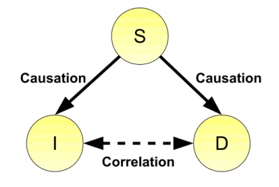
A common example to illustrate the problem is the relationship between eating ice cream in summer and drowning deaths. Plotting the number of people who drowned against ice cream sales over the period of one or several years, we might infer that eating ice cream causes drowning. But if we have a closer look to our example we will find that we did not take the season and the air temperature into account. Assume that ”I” is the variable for the ice cream sales, ”D” represents the variable for the number of drowning deaths and ”S” describes the season or air temperature. Although we find a correlation between
”I” and ”D”, we find that ”I” and ”D” are independent given ”S” (see Figure 1.2). This illustrates one of the main pitfalls in causal inference: the third common cause.
D I
S
Causation Causation
Correlation
Figure 1.2: The third common cause. The observed correlation between I and D is not due to a direct causal connection between I and D, but due to a third common cause S, which has a causal effect on both I and D.
Another common problem is to infer the direction of causal effects between two variables.
Assume there is an alien which just arrived on earth for research and this alien is attracted
by fire. Every time it observes a fire it also observes firemen. Since the alien does not know about the function of a fire brigade it might assume that these firemen are the cause of these fires, which is obviously not the case.
In summary a correlation between two variables X and Y may imply that
• X causes Y or
• Y causes X or
• there is a third common factor, which causes both X and Y or
• X and Y cause each other in a feedback loop or
• we observe a pure coincidence.
What does that mean for our observational study to detect the causal relationship between smoking and lung cancer of 30 year old women over 10 years? Imagine there is a gene which makes smoking highly attractive for some women and now imagine that the same gene directly causes lung cancer. Then we have an unobserved third common cause in our observational study and would maybe draw a completely different conclusion, if we include this cause into our study. In the early 1950ties Professor Bradford Hill and Dr. Richard Doll came up with some studies which described a connection between smoking and developing lung cancer (Doll and Hill, 1950, 1952, 1954, 1956). Their observational studies showed that there are more smokers among the patients with lung cancer than among other patients. Thus, they concluded that smoking plays an important role in developing lung cancer. However, the famous statistician Ronald Fisher strongly criticized these studies, since correlation never implies causation and there might be other reasons like a third common cause, which might explain the observed correlation (Fisher, 1958a,b,d,c).
And indeed, even if there are chemical mechanisms known today, which link smoking and the risk of developing lung cancer (Hecht, 2002), there are also studies which identified a genetic disposition for developing lung cancer (Amos et al., 2008; Hung et al., 2008;
Thorgeirsson et al., 2008). However, today there is a general consensus among scientists and physicians, that smoking is a major risk factor for smoking (Torre et al., 2016; Cheng et al., 2016; Swanton and Govindan, 2016; Malhotra et al., 2016). And Ronald Fisher not only was a passionate smoker, but also worked as a consultant for the tobacco industry.
But he showed, if causal statements are derived from pure correlation, this offers weak points of the analysis.
Obviously, it is a hard task to uncover causal connections, but sometimes interventional studies cannot be conducted due to ethical aspects even if we know this would be the better choice. In genetic studies there is another reason, why we sometimes have to refer
to an observational instead of an interventional study. Imagine we want to find out the causal effects of 10.000 genes onMYC. This would result in 10.000 interventional studies (one for each gene), which is impossible to handle with reasonable effort in reasonable time. An observational study would need much less effort, but the only information we get is a correlation, which is not causally interpretable.
During this introductory section I will present in detail under which assumptions we can infer causal effects from observational data. I summarize how we can estimate at least an incomplete causal structure from observational data and how we can estimate causal effects from that graph without doing any interventional experiments.
1.2.2 Estimation of causal effects from observational data when the causal structure is known
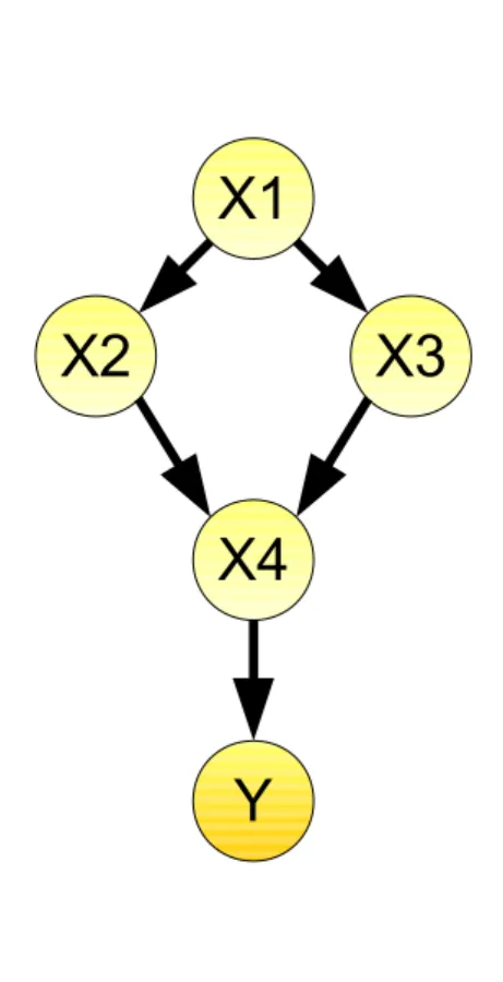
First we need to define a mathematical representation of the causal structure. We assume our causal relationships between genes to be a directed graph consisting of nodes X = X1, ...,Xp and directed edgesE =E1, ...,Es. The directed graph does not contain cycle, and we call the graph directed acyclic graph (DAG). Every gene is represented by one node in the network. Statistically, every node is a random variable whose values indicate the expression levels of a gene. In this section we assume that the causal structure of our problem is known. We call all nodes with incoming edges to a node X parents of X (pa(X)). If a node X has two parents Y and Z, which are not connected to each other, we call this pattern a v-structure and X is called a collider (Pearl, 2009) (Figure 1.3).
Edges represent conditional dependencies; nodes that are not connected represent variables that are conditionally independent. Moreover, we interpret the edges causally.
If there is a directed edge X → Y, we assume that an experimental perturbation of the expression level of X will affect Y, but not vice versa. This causal interpretation is ensured by the Causal Markov condition first described by Kiiveri and Speed (1982).
The Causal Markov condition is defined as follows:
Definition 1.2.1 (Causal Markov condition by Spirtes, Glymour and Scheines, section 3.4.1, p. 53 (Spirtes et al., 2000) ) Let G be a causal graph with a set of vertices V and let P be a probability distribution over the vertices in V generated by the causal structure represented in G. G and P satisfy the Causal Markov Condition if and only if for every X in V, X is independent of V\(Descendants(X)∪pa(X) ) given pa(X).
In other words: every observation of a gene X is statistically independent of all other genes which are no descendents of X in the causal graph given the parents of X (X
⊥ ⊥
Y|pa(X), with Y =V \(Descendants(X)∪pa(X))).Y X4
X3 X2
X1
Figure 1.3: Example of a DAG.The DAG consists of 5 nodes and 5 edges. The node X1 is the parent of X2 and X3, X2 and X3 are the parents of X4 and X4 is the parent of Y. X2, X3 and X4 form a v-structure and X4 is the collider of this v-structure.
To determine all statistical independencies of a DAG and, thus, to characterize a set of distributions which is compatible with that DAG we can apply the d-separation criterion:
Definition 1.2.2 (d-Separation by Judea Pearl, definition 1.2.3, p. 16, (Pearl, 2009) )A path p is said to be d-separated (or blocked) by a set of nodes Z if and only if i p contains a chain i → m → j or a fork i ← m → j such that the middle node m
is in Z, or
ii p contains an inverted fork (or collider) i → m ← j such that the middle node m is not in Z and such that no descendant of m is in Z.
A set of nodes Z is said to d-separate X from Y if and only if Z blocks every path from a node in X to a node in Y.
The converse of the Causal Markov Condition, the causal faithfulness condition en- sures that all conditional independencies observed are due to the Causal Markov condi- tion:
Definition 1.2.3 (Causal Faithfulness condition by Spirtes, Glymour and Scheines, section 3.4.3, p. 56 (Spirtes et al., 2000) ) Let G be a causal graph and P a prob- ability distribution generated by G. G and P satisfy the Causal Faithfulness Condition if and only if every conditional independence relation true in P is entailed by the Causal Markov condition applied to G.
A violation of this property is possible if for example the observations of two different genes are connected by two different paths, which cancel each other out exactly. Thus, we observe an independence (the causal effect is zero) even though the nodes are causally connected.
For now we assume that we know the causal structure. Given this causal structure and the observations of the genes, we want to determine the causal effect of a gene X on another gene Y. More precisely we want to perturb the gene X and we want to observe what happens to gene Y due to this intervention. However, we do not want to do this in the wet lab. We want to perform a purely computational virtual intervention experiment.
Goldszmidt and Pearl (1992) introduced a new operator to probability theory to allow for such an external intervention called the do-operator. The do-operator do(X = x∗) sets the variable X to a fixed value x∗ and as a result X does not depend on its former parents anymore. But how do we calculate the causal effect of a variable X on a variable Y using this do-operator? Pearl (1993) introduced a graphical criterion called the back- door criterion which provides the link between his do-operator and standard statistical calculus.
Definition 1.2.4 (back-door criterion by Judea Pearl, definition 3.3.1, p. 79, (Pearl, 2009))A set of variablesZ satisfies the back-door criterion relative to an ordered pair (X, Y) in a DAG G, if
(i) no node in Z is a descendant of X.
(ii) Z blocks (see def. 1.2.2 ) every path between X and Y that contains an arrow into X.
Pearls back-door adjustment enables the calculation of the causal effect:
Definition 1.2.5 (back-door adjustment by Judea Pearl, theorem 3.3.2, p. 79, (Pearl, 2009))If a set of variables Z satisfies the back-door criterion relative to (X, Y), then the causal effects of X on Y is identifiable and is given by the formula P(Y|X = do(X =x∗)) =P
ZP(Y|X, Z)P(Z).
Further, it can be shown, that the true parents of a nodeXdo always fulfill the Back-door criterion relative to every ordered pair (X, Y) (Pearl, 2009). We see
P(Y|do(X =x∗)) =
P(Y) :Y ∈paX
R P(Y|X =x∗, paX)P(paX) dpaX :Y /∈paX.
(1.1)
Following Rosenbaum and Rubin (1983), Maathuis et al. (2009) defined the difference E(Y|do(X =x∗))−E(Y|do(X =x∗∗)) as ”causal effect”.
E(Y|do(X =x∗)) = Z
Y ·P(Y|do(X =x∗)) dy :(1.2)
=
R Y ·P(Y) dy :Y ∈paX
R R Y ·P(Y|X =x∗, paX)P(paX) dpaXdy :Y /∈paX. (1.3)
=
E(Y) :Y ∈paX
R R Y ·P(Y|X =x∗, paX) dyP(paX) dpaX :Y /∈paX. (1.4)
=
E(Y) :Y ∈paX
R E(Y|X =x∗, paX)P(paX) dpaX :Y /∈paX.
(1.5)
=
E(Y) :Y ∈paX
R E(Y|X =x∗, paX)P(paX) dpaX :Y /∈paX.
(1.6)
We further assume our variables to be multivariate Gaussian and we conclude
E(Y|X =x∗, paX) =β0+βxX+βpaTXpaX. (1.7)
In summary βX from
Y =β0+βXX+βpaTXpaX +:Y /∈paX, (1.8) is a consistent estimator of the causal effect of X on Y (Maathuis et al., 2009). If Y ∈paX the causal effect ofX onY is zero. The parents of X,paX, adjust the regression for possible confounders that affectX and Y simultaneously, which could create spurious correlations between X and Y. Note that there might be other sets of variables Z that also fulfill the back-door criterion and can be used in the regression above instead of the setpaX.
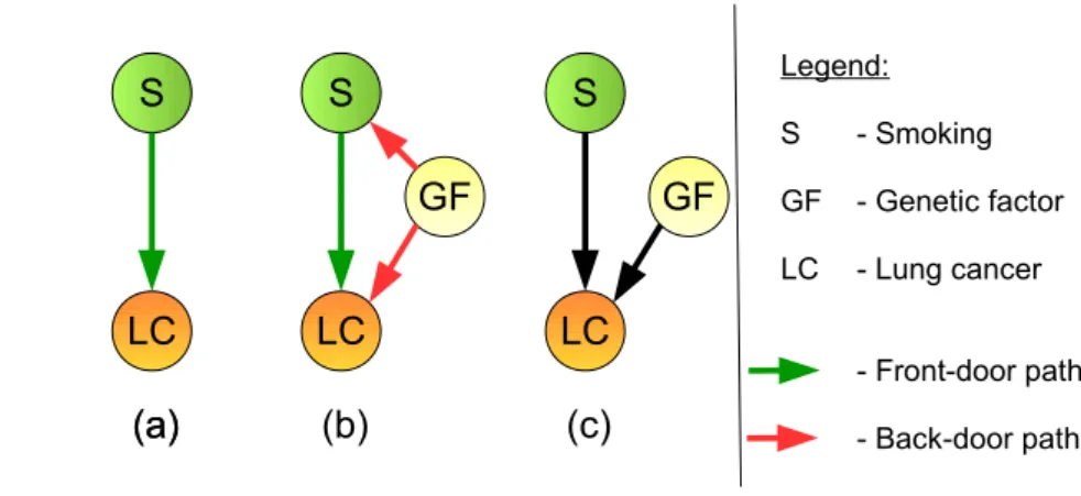
This basis might help to solve the ”smoking - lung cancer problem”. The surgeons from Doll and Hill (1950, 1952, 1954, 1956) claim that there is a direct effect between smoking and lung cancer, which is shown by the graph in Figure 1.4 (a), while Fisher would answer that there might be a third common cause, e.g. a genetic factor influencing both, the urge to smoke and a higher probability of getting lung cancer as shown in Figure 1.4 (b). If the genetic factor influencing both could be observed, the causal effect can be calculated by applying the back-door criterion. The back-door criterion aims to close all back-door paths (Figure 1.4 (b), red arrows), while leaving the front-door paths (Figure 1.4 (b), green arrows) open. The causal effect of smoking on getting lung cancer differs depending on the presence or absence of the genetic factor. Closing the back-door paths means to take out the variation due to the genetic factor and to compare people with the same genetic factor to each other which is equivalent with holding the genetic factor constant. Thus, the causal effect observed does not depend on the influence of the genetic factor on smoking anymore, since we control for this variable. However, if the genetic factor is unobserved, the back-door criterion cannot be applied and the problem is more complicated. Pearl (2009) offers another graphical criterion which still helps solving the problem. He introduces another variable ”tar deposit in the lung” and applies the front-door criterion to calculate the causal effect.
1.2.3 Causal structure learning
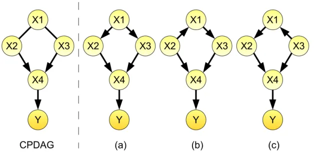
In the previous section we assumed that the causal DAG of the problem is known. A DAG fully specifies the conditional dependencies of all nodes (Pearl, 1988), but not vice versa. Several DAGs with the same skeleton of undirected edges and the same v-structures (Pearl, 2009) encode the same conditional dependency structure (Verma and Pearl, 1990).
These equivalence classes of DAGs can be represented by completed partially directed acyclic graphs (CPDAGs) that consist of the joint skeleton and the directed edges which
(b) (c) LC
GF S
LC GF
S Legend:
S - Smoking GF - Genetic factor LC - Lung cancer
- Front-door path - Back-door path
(a) LC S
(a)
Figure 1.4: The back-door criterion for the ”smoking - lung cancer problem”.
(a) Model which assumes a direct causal effect between smoking and developing lung cancer. (b) Model which assumes a third common cause, a genetic factor, which influences both the urge to smoke and the probability of getting lung cancer. Green arrows show the front-door paths, red arrows show the back-door paths. (c) Application of the back-door criterion to subfigure (b) with the aim to examine whether smoking causes lung cancer.
are common to all DAGs in the equivalence class (Chickering, 2002a). In many scenar- ios, especially in biology, neither the DAG nor the CPDAG are known. For example, the causal gene regulatory networks which explain the emergence of cancer are widely unknown. Thus, we need to estimate the causal structure from the data we observe.
However, causal structure learning is NP hard (Chickering et al., 2004). For a set of n vertices we can find 2n(n−1) possible directed networks (Harary and Palmer, 1973), e.g.
for 5 nodes there are 1.048.576 possible directed graphs.
Fortunately there is a huge amount of methods, which provide solutions. Structure learning algorithms are divided into 3 main groups: (i)”search and score”, (ii)”constraint- based” and (iii)”hybrid” algorithms (Daly et al., 2011). Search and score methods require a score to determine how well the (estimated) graph fits the data. This scoring function is optimized by a search algorithm. Several scoring functions might be used, for example the Likelihood (Cooper and Herskovits, 1992), the Bayesian Information Criterion (BIC) (Schwarz et al., 1978) or the Akaike Information Criterion (Akaike, 1974). Examples for score and search algorithms are the Markov chain Monte Carlo model composition algo- rithm (Madigan et al., 1995), the Sparse Candidate algorithm (Friedman et al., 1999), the optimal reinsertion algorithm (Moore and Wong, 2003), Genetic algorithms (Larra˜naga et al., 1996a,b; de Campos and Huete, 2000; Wong and Leung, 2004; Gao et al., 2007) or the Greedy Search algorithm (Chickering, 2002b).
Even if there are some search and score methods for causal inference (Heckerman, 1995), the majority of causal structure learning methods are constraint based methods (Daly et al., 2011). Constraint based algorithms use conditional independencies (CIs) to ex-
plore the network structure. These CIs are explored by statistical independence tests on triples X, Y and Z, where X and Y are single variables and Z describes a subset of nodes in the network. If X and Y are independent given the set Z (X
⊥ ⊥
Y|Z), then the edge from X to Y is removed from the graph. In general constraint based methods are much faster than search and score methods. Testing whether X⊥ ⊥
Y|Z requires looking at the variables X, Y and Z while changing an edge in a score based method means that we need to calculate a score over all variables in the network. Spirtes and Glymour (1991) developed one of the most common constraint based algorithms, the PC algorithm. It consists of two steps: the first step, which estimates the skeleton of the network and the second step, where the v-structures are calculated and some further orientation rules are applied to orient the edges. The parameter α of the PC algorithm influences the sparseness of the estimated network, such that larger values ofα increase the number of edges in the network. However, the PC algorithm cannot direct all edges since different networks with identical skeletons can encode the same conditional independence assump- tions and thus can not be distinguished on observational data only (Verma and Pearl, 1990). The result of the PC algorithm is the equivalence class of graphs represented by a CPDAG. Kalisch and B¨uhlmann (2007) showed that the PC algorithm is statistical consistent and feasible for high-dimensional data up to thousands of variables as long as the underlying DAG is sparse. The PC algorithm is order-dependent, which means, that the result of the algorithm depends on the ordering of the variables, since this ordering determines the statistical tests to be made. But Colombo and Maathuis (2014) proposed some modifications of the PC algorithm to overcome of this order-dependence in parts.Hybrid methods combine the concepts of ”search and score” and ”constraint based” meth- ods. The Max-Min Hill-Climbing (MMHC) algorithm from Tsamardinos et al. (2006) is a widely known representative of this class of structure learning algorithms. The first part of the MMHC algorithm uses the constraint-based MMPC algorithm (Tsamardinos et al., 2003) to reconstruct the skeleton of the graph, while in the second step a ”search and score” strategy orients the edges based on the skeleton. An algorithm based on the MMHC algorithm proposed by N¨agele et al. (2007) allows the estimation of networks with ten thousands of variables. This algorithm focuses on the Markov Blankets of each node. A Markov Blanket is a special subgraph around a certain node, that contains all other nodes of the graph, which are necessary to predict the behavior of that node and its parents (Pearl, 1988). This variation of the MMHC algorithm estimates the Markov Blan- kets around each variable and combines the results. The key benefit of this substructure learning is the possibility to parallelize the estimation of Markov Blankets.
1.2.4 Estimation of causal effects from observational data with unknown causal structure
Section 1.2.2 describes how to estimate causal effects from observational data, when the causal structure is known, and section 1.2.3 discusses the possibilities to estimate a causal structure from observational data. In this section, I introduce ”Intervention calculus when the Directed acyclic graph is Absent” (IDA, Maathuis et al. (2009, 2010)), which combines these two ideas. IDA consists of two steps: First the PC algorithm estimates a CPDAG from the observational data (Kalisch and B¨uhlmann, 2007) and then Pearl’s do calculus (Pearl, 2009) is used to estimate the causal effects from observational data using the estimated CPDAG in the second step. Since Maathuis et al. (2009) assume Gaussianity the causal effect is estimated using equation 1.8. But there are undirected edges in a CPDAG and this complicates the estimation of causal effects. However, the approach of Maathuis et al. (2009) allows to estimate lower bounds of the effect size. The IDA algorithm first enumerates all possible parent sets of a nodeX and then calculates causal effects of X on the targets of interest for each of the possible parent sets by equation 1.8.
Thus, IDA estimates not necessarily exactly one, but a multiset of causal effects for each ordered pair X and Y (see Figure 1.5 for an example). The minimum absolute value of this multiset provides a lower bound of the absolute effect size. Maathuis et al. (2010) show in applications that IDA outperforms regression-based methods in terms of number of true positives versus number of false positives for the top 5000 predicted effects on the transcriptome of yeast gene deletion strains from a large dataset of expression profiles of wild type yeast. However, in simulations with large networks and medium sized datasets, which are typical for many biological applications, networks often cannot be reconstructed correctly. Meinshausen and B¨uhlmann (2010) suggest stability selection, a subsampling strategy that is wrapped around IDA as a remedy. K subsets of the data are drawn and for each of these subsets IDA estimates the lower bound of the effects. Finally, the effects are ranked by how often they appear in the top q effects. This procedure is further improved by the CStaR algorithm of Stekhoven et al. (2012) which repeats stability selection for several values of q and the median rank over different values of q is used to calculate the final rank of a causal effect. The CStaR algorithm outperforms plain IDA with respect to true positive selections versus false positive selections (Stekhoven et al., 2012).
1.3 Outline
The thesis is organized in two parts:
Y X4
X3 X2
X1
Y X4
X3 X2
X1
Y X4
X3 X2
X1
Y X4
X3 X2
X1
CPDAG (a) (b) (c)
Figure 1.5: A CPDAG and its accompanying DAGs. There are three DAGs ((a)-(c)) belonging to the CPDAG on the left. If we are interested in the causal effect of X1 on Y, IDA calculates the multiset of three causal effects of X1 on Y according to the three DAGs corresponding to the CPDAG. In DAG (a) X1 has no parents and the causal effect of X1 on Y is βX1 from Y =β0+βX1X1 +. The parent of X1 in DAG (b) is X2 and thus the causal effect of X1 on Y is βX1 fromY = β0 +βX1X1 +βX2X2 + and similarly the causal effect of X1 on Y is βX1 from Y =β0+βX1X1 +βX3X3 + for DAG (c). The minimum absolute value of these thee causal effects is a lower bound for the effect size.
Part1: In this methodological part I derive methods to work on the following three issues:
First,MYC is an transcriptional amplifier and we have to account for that during exper- imental design. There are already methods described in Section 1.1.3 that deal with that problem in transcriptomics, but these methods do not account for variability in cell lysis during RNA extraction. Thus, I introduce a new calibration method for gene expres- sion data measured under transcriptional amplification. This method uses spike-in cells fromDrosophila melanogaster to calibrate samples from different amounts of total RNA (Taruttis et al., 2017). In comparison to the usage of the ERCC spike-in set described in Section 1.1.3 the proposed method not only accounts for cell lysis effects but is also cheaper and easier to handle than the ERCC spike-ins.
Second, causal inference from observational data is a hard task. From the introducing Section 1.2 we know that there are already methods for the estimation of causal effects from observational data and that a subsampling approach is highly recommended. How- ever the described methods only estimate a lower bound of the causal effects and do not use the causal effects of all multi sets. The method I propose is called accumulation IDA (aIDA) and uses the mode of the distribution of causal effects to generate the causal effect from the effects estimated from the subsampling runs. This advancement provides an improvement of the already existing methods.
Third, an assumption of these causal inference methods is that the data underlying graph is sparse. SinceMYC is a transcriptional amplifier the graph underlying a dataset which includes the geneMYC is very likely not sparse, sinceMYC influences nearly every gene in the dataset. The spike-in calibration methods help to uncover this dense structure in a transcriptomic dataset. Computationally, the calibration of the data using a spike-in method will result in highly correlated data. So far it is unclear how to deal with this high dependencies since they violate the assumption that the underlying graph is sparse.
I try to improve the estimation of causal effects from highly correlated observational data by replacing the PC algorithm with a version of the MMHC algorithm.
Part II: Part II applies the algorithms and methods developed in Part I to a data set, which is appropriate to examine the causal connections around MYC. The data set consists of transcriptomic and metabolomic data to unravel causal connections between genes and metabolites. I calibrate the RNA-seq data using the whole spike-in method presented in section 2.4, which results in highly correlated data. Thus, I estimate the causal effects of the genes on the metabolites and the causal effects between genes using the MMHC-aIDA algorithm described in section 4.4, since it shows a better performance on highly correlated data. Whereas aIDA (section 3.4) estimates the causal effects of