Estimation of Dose Distribution for Lu-177 Therapies in Nuclear Medicine

(1)

Estimation of Dose Distribution for Lu-177 Therapies in Nuclear Medicine

Inaugural-Dissertation zur Erlangung der Doktorwürde der Fakultät für Sprach-, Literatur und Kulturwissenschaft

der Universität Regensburg vorgelegt von

Dr. rer. nat. Theresa Ida Götz

aus Weiden in der Oberpfalz

2020, Fakultät für Sprach-, Literatur und Kulturwissenschaft

Die Arbeit entstand in gemeinsamer Betreuung durch die Fakultät für Physik der Universität Regensburg und der Fakultät für Medizin der

Friedrich-Alexander-Universität Erlangen-Nürnberg

Regensburg, 2020

(2)

Erstgutachter (Betreuer): Prof. Dr.-Ing. Bernd Ludwig Zweitgutachter: Prof. Dr. Elmar Wolfgang Lang

Drittgutachter: PD Dr. David Elsweiler

(3)

Abstract

In nuclear medicine, two frequent applications of

¹⁷⁷

Lu therapy exist: DOTATOC therapy for patients with a neuroendocrine tumor and PSMA thearpy for prostate cancer. During the therapy a pharmaceutical is injected intravenously, which at- taches to tumor cells due to its molecular composition. Since the pharmaceutical contains a radioactive

¹⁷⁷

Lu isotope, tumor cells are destroyed through irradiation.

Afterwards the substance is excreted via the kidneys. Since the latter are very sen- sitive to high energy radiation, it is necessary to compute exactly how much ra- dioactivity can be administered to the patient without endangering healthy organs.

This calculation is called dosimetry and currently is made according to the state of the art MIRD method. At the beginning of this work, an error assessment of the established method is presented, which has determined an overall error of 25% in the renal dose value. The presented study improves and personalizes the MIRD method in several respects and reduces individual error estimates considerably.

In order to be able to estimate of the amount of activity, first a test dose is injected to the patient. Subsequently, after 4h, 24h, 48h and 72h SPECT images are taken. From these images the activity at each voxel can be obtained a specified time points, i. e. the physical decline and physiological metabolization of the pharmaceutical can be followed in time. To calculate the amount of decay in each voxel from the four SPECT registrations, a time activity curve must be integrated.

In this work, a statistical method was developed to estimate the time dependent activity and then integrate a voxel-by-voxel time-activity curve. This procedure results in a decay map for all available 26 patients (13 PSMA/13 DOTATOC).

After the decay map has been estimated, a full Monte Carlo simulation has been carried out on the basis of these decay maps to determine a related dose distribution. The simulation results are taken as reference (“Gold Standard”) and compared with methods for an approximate but faster estimation of the dose dis- tribution. Recently, a convolution with Dose Voxel Kernels (DVK) has been estab- lished as a standard dose estimation method (Soft Tissue Scaling STS). Thereby a radioactive Lutetium isotope is placed in a cube consisting of soft tissue. Then radiation interactions are simulated for a number of 10

¹⁰

decays. The resulting Dose Voxel Kernel is then convolved with the estimated decay map. The result is

3

(4)

a dose distribution, which, however, does not take into account any tissue density differences. To take tissue inhomogeneities into account, three methods are de- scribed in the literature, namely Center Scaling (CS), Density Scaling (DS), and Percentage Scaling (PS). However, their application did not improve the results of the STS method as is demonstrated in this study. Consequently, a neural net- work was trained finally to estimate DVKs adapted to the respective individual tissue density distribution. During the convolution process, it uses for each voxel an adapted DVK that was deduced from the corresponding tissue density kernel.

This method outperformed the MIRD method, which resulted in an uncertainty of the renal dose between −42.37 −10.22% an achieve a reduction in the uncertainty to a range between −26.00% − 7.93%. These dose deviations were calculated for 26 patients and relate to the mean renal dose compared with the respective result of the Monte Carlo simulation. In order to improve the estimates of dose distri- bution even further, a 3D 2D neural network was trained in the second part of the work. This network predicts the dose distribution of an entire patient. In combi- nation with an Empirical Mode Decomposition, this method achieved deviations of only −12.21% − 2.13% . The mean deviation of the dose estimates is in the range of the statistical error of the Monte Carlo simulation.

In the third part of the work, a neural network was used to automatically seg-

ment the kidney, spleen and tumors. Compared to an established segmentation

algorithm, the method developed in this work can segment tumors because it uses

not only the CT image as input, but also the SPECT image.

(5)

Zusammenfassung

In der Nuklearmedizin gibt es zwei Anwendungen einer

¹⁷⁷

Lu-Therapie, zum einen die DOTATOC-Therapie für Patienten mit einem neuroendokrinen Tumor und zum anderen die PSMA-Thearpie für Prostatakrebs. Bei dieser Therapieform wird intravenös ein Stoff gespritzt, welcher sich aufgrund der molekularen Zusam- mensetzung an Tumorzellen anlagert. Da an die Moleküle ein radioaktives Lu- Isotope gekoppelt ist, werden so Tumorzellen durch die Bestrahlung getötet. Mit der Zeit wird der Stoff über die Nieren ausgeschieden. Da es sich bei den Nieren um ein strahlen-sensitives Organ handelt, muss vor der Injektion genau berechnet werden, wie viel Aktivität dem Patienten gespritzt werden kann, ohne die gesun- den Organe zu gefährden. Diese Berechnung nennt man Dosimetrie und wird laut Stand der Technik mittels MIRD Verfahren durchgeführt. Zu Beginn dieser Arbeit wird eine Fehlerabschätzung der etablierten Methode vorgestellt, welche einen Gesamtfehler von 25% beim Nierendosiswert ermittelt hat.

Um eine Abschätzung der Aktivitätsmenge treffen zu können, wird dem Pa- tienten zunächst eine Testdosis gespritzt. Anschließend werden nach 4h, 24h, 48h und 72h SPECT-Bilder aufgenommen. Aus den Bildern kann die Aktivität pro Voxel zu einen gewissen Zeitpunkt abgelesen werden. Um nun aus den vier Mo- mentaufnahmen zu berechnen, wie viel Zerfälle pro Voxel stattgefunden haben, muss über eine Zeit-Aktivitätskurve integriert werden. In dieser Arbeit wurde ein statistisches Verfahren entwickelt, um eine voxelweise Zeit-Aktivitätskurve abzuschätzen und anschließend zu integrieren. Resultat dieses Verfahrens ist eine Zerfallskarte für jeden der 26 vorhandenen Patienten (13 PSMA/13 DOTATOC).

Nachdem die Zerfallskarte berechnet wurde, kann anhand dieser eine volle Monte Carlo Simulation erfolgen, welche eine Dosisverteilung ermittelt. Diese wird als Gold Standard angenommen und mit den Verfahren zur schnelleren Ab- schätzung der Verteilung verglichen. Als Standard Methode (Soft Tissue Scaling STS) wurde eine Faltung mit einem Dose Voxel Kernel (DVK) publik. Dabei wird in einem Würfel bestehend aus Weichteilgewebe ein Lutetium-Isotope platziert, anschließend werden 10

¹⁰

Zerfälle simuliert. Der resultierende Dose Voxel Ker- nel wird dann mit der Zerfallskarte gefaltet. Resultat ist eine Dosisverteilung, welche jedoch keine Dichteunterschiede berücksichtigt. Um Letztere zu berück-

5

(6)

sichtigen, existieren in der Literatur drei Methoden, nämlich Center Scaling (CS), Density Scaling (DS) und Percentage Scaling (PS). Diese erzielten jedoch in dem in der Arbeit durchgeführten Vergleich keine Verbesserung zur STS Methode.

Um auf die jeweilige Dichteverteilung angepasste DVKs abzuschätzen, wurde ein neuronales Netz trainiert. Dieses verwendet während des Faltungsprozess für jeden Voxel einen anderen DVK, der für diesen Dichtekernel vorhergesagt wurde. Durch diese Methode konnte statt −42.37% − 10.22% Abweichung in der Nierendosis eine reduzierte Range von −26.00% − 7.93% erzielt werden. Die Abweichungen sind ein Mittelwert über 26 Patienten und betreffen die mittlere Nierendosis im Vergleich mit der Monte Carlo Simulation. Um die Schätzungen der Dosisverteilung noch zu verbessern, wurde im zweiten Teil der Arbeit ein 3D- 2D-Neural-Network trainiert. Dieses Netz sagt die Ganzkörper-Dosisverteilung eines gesamten Patienten vorher. In Kombination mit einer Empirical Mode De- composition erzielte diese Methode Abweichungen von nur −12.21% − 2.13%.

Diese mittlere Abweichung der Dosisschätzungen liegt im Bereich des statistis- chen Fehlers der Monte Carlo Simulation.

Im dritten Teil der Arbeit wurde ein Neuronales Netz verwendet um automa-

tisiert die Niere, Milz und Tumore zu segmentieren. Im Vergleich zu einem

etablierten Segmentierungsalgorithmus kann die in dieser Arbeit entwickelte Meth-

ode Tumore segmentieren, da sie nicht nur das CT Bild als Eingabe verwendet,

sondern auch das SPECT Bild.

(7)

Abbreviations

SPECT/CT Single-Photon Emission Computed Tomography / CT PET/CT Positron-Emission Tomography / CT

SPECT Single-Photon Emission Computed Tomography PET Positron-Emission Tomography

CT Computed Tomograpy

MIRD Medical Internal Radiation Dose Committee DVK Dose Voxel Kernel

DPK Dose Point Kernel MC Monte Carlo Simulation NET Neuroendocrine tumor

ADT Androgen Deprivation Therapy

PRRT Peptide Radionuclide Receptor Therapy

mCSPC metastatic castration-sensitive Prostate Cancer (PC) mCRPC metastatic castration-resistant PC

SSTR Somatostatin Receptor TTD Total Tumor Dose PC Prostate Cancer

PSMA Prostate Specific Membrane Antigen TAC Time Activity Curve

EM Expectation Maximization TIA Time Integrated Activity VOI Volume Of Interest

OLINDA Organ Level Internal Dose Assessment with Exponential Modeling SE Standard Error

SD Standard Deviation SS Sample Size

PF Particle Filter

SNR Signal to Noise Ratio DNN Deep Neural Networks

EMD Empirical Mode Decomposition

EEMD Ensemble Empirical Mode Decomposition

11

(12)

MEEMD Multi-dimensional Ensemble Empirical Mode Decomposition BEMD Bi-Dimensional EMD

CNN Convolutional Neural Network IMF Intrinsic Mode Function

BIMF Bi-dimensional Intrinsic Mode Function

BEEMD Bi-dimensional Ensemble Empirical Mode Decomposition (EEMD) GiT-BEMD Green’s function in Tension - Bi-dimensional EEMD (BEEMD) BIM Bi-dimensional Intrinsic Mode

MLE Maximum Likelihood Estimation ReLU Leaky Rectified Linear Units MLP Multi-Layer Perceptrons LCN Local Contrast Normalization SGD Stochastic Gradient Descent KL Kullback-Leibler divergence CgA Chromogranin A

PSA Prostate Specific Antigen AUC Area Under the Curve SEM State Evolution Model OM Observation Model HU Hounsfield Units STS Soft Tissue Scaling CS Center Scaling DS Density Scaling PS Percentage Scaling

DVK-NN DVK via Neural Networks NN Neural Network

DE-NN-EMD Dose Estimation via Neural Network and EMD DE-NN Dose Estimation via Neural Network

LOOCV Leave-One-Out Cross-Validation RLT Radioligand Therapy

FBP Filtered Back-Projection

SIR Sampling Importance Resampling PCA Principal Component Analysis

CMSC Comparable Minimal Scale Combination Principle

GT Ground truth

(13)

Introduction

More and more therapies with radiopharmaceuticals, labeled with beta emitting isotopes, are established, making the need for a patient-specific dosimetry of fun- damental importance [22, 157, 55]. With the aid of hybrid Single-Photon Emis- sion Computed Tomography / CT (SPECT/CT) and Positron-Emission Tomogra- phy / CT (PET/CT) imaging techniques, it is possible to obtain tissue density information in conjunction with the distribution of radioactivity inside the human body. The spatial resolution of nuclear medicine imaging of such activity distri- butions is in the mm to cm range. Consequently, macroscopic non-uniformities in the activity distribution can be detected. In [141, 53] an overview of imaging- based patient-specific dosimetry methods is given.

First of all, a spatial distribution of radioactivity over time using the patient’s own anatomy is needed to obtain as output the spatial distribution of absorbed energy dose. [142, 69] A well-known dosimetry method is the calculation of S-values according to the Medical Internal Radiation Dose Committee (MIRD) formalism, where a standard phantom is defined [121]. The aim of this work is to obtain a patient specific dosimetry by using Dose Voxel Kernel (DVK).

The energy dose produced in a specific volume can be calculated as the linear superposition of contributions from each voxel (volume element) in the spatial activity distribution treated as a radiation point source. The energy dose produced by a radiation point source of isotropic unit activity in a homogeneous medium of infinite extension is called a Dose Point Kernel (DPK) [119, 18]. A number of publications compare DPK data bases generated with different Monte Carlo Simu- lation (MC) softwares such as GATE, FULKA, MCNP4C, CGSnrc and GEANT4 [115, 22]. The generally considered tissues are bone, lung, soft tissue and water.

All data bases contain DPKs for the radioactive isotopes Iodine

¹³¹

I and Yttrium

90

Y . Instead of calculating a continuous DPK, a discrete DVK, also called S-voxel kernel, can be determined [113, 114]. The voxel size can be chosen arbitrarily, because the kernel can be scaled, as shown in [113, 125, 42]. To obtain the dis- tribution of absorbed energy dose based on the patient’s anatomy, the decay map has to be convolved with the DVK.

The estimation of DVKs is hardly explored in literate, yet some studies are

13

(14)

reported. Dieudonne at al. [36] report a comparison of dose estimations obtained with either a full MC simulation or by convolution with a DVK. The latter was computed for homogeneous soft tissue only and results have been reported for two patient specific dose estimations. In contrast, Scarinci et al. [137] com- puted DVKs for several tissues, but did not provide any comparison to the stan- dard MIRD method. Hence possible improvements cannot be quantified, limiting the value of this study. Rather than computing DVKs for many tissues, results obtained with soft tissue density kernels could be scaled according to the tissue density under study. Along these lines, Dieudonne at al. [37] proposed that the product of the energy dose per voxel times the mass density of that voxel should be an invariant of the system. This proposal leads to the following density correction:

D

_ρ

(r) · ρ(r) = D

_ST

(r) · ρ

_ST

(1) where D

_ST

(r) = ∂E(r)/ρ

_ST

∂V

_vox

is the dose for one voxel with volume V

_vox

, centered at r = (x, y, z)

^T

, and calculated for soft tissue as the material inside the voxel, ρ(r) is the voxel mass density, D

_ρ

(r) is the density-corrected voxel dose value and ρ

_ST

= 1040 kg/m

³

is the mass density of soft tissue. This density scal- ing of absorbed energy dose was demonstrated on three different clinical cases.

In each case, three different dose estimation methods were employed: a full MC simulation of the DVK, a convolution of the TIA map with a soft tissue DVK and finally a convolution with a density-scaled DVK

In yet another recent study, the DVKs where first scaled according to the en- ergy dose distribution calculated in different tissues, and then convolved with the activity distribution. The aim was to take into account interface regions, where the mass density changes abruptly. This method is evaluated on the Zubal phantom for three different dose distributions. [76].

Similarly, the aim of the work reported in [100] was to evaluate the appli-

cation of tissue-specific dose kernels instead of water dose kernels to improve

the accuracy of patient-specific dosimetry by taking tissue heterogeneities into

consideration. Tissue-specific DPKs and DVKs for Yttrium-90 (

⁹⁰

Y ), Lutetium-

177 (

¹⁷⁷

Lu), and Phosphorus-32 (

³²

P ) were calculated using the MC code GATE

(version 7). The calculated DPKs for bone, lung, adipose, breast, heart, intestine,

kidney, liver, and spleen are compared with those of water. The dose distribu-

tion in normal and tumorous tissues in lung, liver, and bone of a Zubal phan-

tom was calculated using tissue-specific DVKs instead of those of water in con-

ventional methods. For a tumor defined in a heterogeneous region in the Zubal

phantom, the absorbed dose was calculated using a proposed algorithm, taking

tissue heterogeneity into account. The algorithm was validated against full MCs

and indicated that the largest differences between water and other tissue-specific

(15)

CONTENTS 15 DPKs occurred in bone, whereby the difference amounted to

⁹⁰

Y : 12.2 ± 0.6 %,

32

P : 18.8 ± 1.3 %, and

¹⁷⁷

Lu : 16.9 ± 1.3 %. The second largest discrep- ancy corresponded to the lung with

⁹⁰

Y : 6.3 ± 0.2 %,

³²

P : 8.9 ± 0.4 %, and

177

Lu : 7.7 ± 0.3 %. For

⁹⁰

Y , the mean absorbed dose in tumorous and nor- mal tissues was calculated using tissue-specific DVKs in lung, liver, and bone.

The results were compared with doses calculated considering the Zubal phantom water equivalent and the relative differences were 4.50%, 0.73%, and 12.23%, re- spectively. For the tumor in the heterogeneous region of the Zubal phantom that includes lung, liver, and bone, the relative difference between mean calculated dose in tumorous and normal tissues based on the proposed algorithm and the val- ues obtained from full MC dosimetry was 5.18%. The authors concluded that their algorithm potentially enabled patient-specific dosimetry and improved estimates of the average absorbed dose of Yttrium-90 in a tumor located in lung, bone, and soft tissue interface by 6.98% compared with the conventional methods.

In [93] it was pointed out that the aim of personalized radiotherapy is clearly expressed in the EU directive 2013/59/EURATOM Article 56:

For all medical exposure of patients for radiotherapeutic purposes, exposures of target volumes shall be individually planned and their delivery appropriately verified taking into account that doses to non-target volumes and tissues shall be as low as reasonably achievable and consistent with the intended radiotherapeutic purpose of the exposure.

This statement formulates the goals onto which this thesis will also concen-

trate, namely first an individual planning of radiation energy delivery and second

a verification of the energy dose absorbed in the target volume.

(16)

(17)

Chapter 1 Nuclear Medical Physics

1.1 ¹⁷⁷ Lu radionuclide therapies

In the department of nuclear medicine of the University Hospital Erlangen, two radionuclide therapies are routinely performed with

¹⁷⁷

Lu - labeled molecules.

These therapies provide a treatment either for Neuroendocrine tumor (NET)s or for PC. In this work, the dose values for both diseases were evaluated.

1.1.1 Neuroendocrine tumors (NETs)

NETs are defined as epithel neoplasms with predominant neuroendocrine differ- entiation that can be observed arising from neuroendocrine cells throughout the body [78]. Data from the Surveillance, Epidemiology, and End Results database suggest that NETs are more prevalent than previously reported with 51% of NETs arising from the gastrointestinal tract, 27% from the lungs and 6% from the pan- creas [169, 170]. NETs of the midgut commonly metastasize to the liver, the mesentery and the peritoneum. Clinically, they are regarded as functional if they are associated with symtoms of hormonal hypersecretion, the so called carcinoid syndrome, or non-functional if they are not associated with hormonal hypersecre- tion [153]. First-line systemic therapy is primarily based on somatostatin analogs which significantly lengthen time to tumor progression and improve control of hormonal secretion [127, 25]. Besides everolimus, a potent inhibitor of mam- malian target of rapamycin, for the treatment of non functional neuroendocrine tumors, so far there have been no standard second-line systemic treatment op- tions [170, 83]. However the recent food and drugs administration approvel of

177

Lu-DOTATATE for the treatment of Somatostatin Receptor (SSTR) positive gastroenteropancreatic tumors, based on the results from the phase 3 Neuroen- docrine Tumors Therapy trial opens new perspectives for the treatment of NETs

17

(18)

[153].

¹⁷⁷

Lu emits beta-particels with a maximum energy of 149 keV , a maxi- mum particle range of 2 mm and has a physical half-life of 6.7 d. Besides beta- particles it also emits gamma photons of 208 keV , which can be directly used for uptake quantification by serial scintigraphy and Single-Photon Emission Com- puted Tomography (SPECT) [47]. Most of the clinical protocols rely on empiri- cal criteria for choosing the administered activity and the number of cycles [20].

Special emphasis has to be placed on the absorbed doses for kidney and bone marrow, since they are considered as the dose limiting organs in

¹⁷⁷

Lu- Peptide Radionuclide Receptor Therapy (PRRT) [133, 162]. Due to the large intrapatient and intralesion variability of tumor uptake in PRRT of NETs [30] it is of utmost importance to improve individualized therapy planning. Therefore methods for accurate dosimetry of tumorous- and non-tumorous tissue and determination of predictive factors that are associated with high uptake of

¹⁷⁷

Lu-DOTATATE in NETs are needed. As yet only a few previously conducted studies reported the use of the MIRD scheme and the unit density sphere model from Olinda for cal- culation of tumor-absorbed doses in

¹⁷⁷

Lu-DOTATATE therapy [30, 67]. The aims of the present study were to evaluate the use of three-dimensional tumor dosimetry based on particle filtering methods and MC to determine the Total Tu- mor Dose (TTD) and to find predictive factors that are associated with a high TTD in patients with SSTR-positive NETs that underwent

¹⁷⁷

Lu-DOTATATE therapy.

1.1.2 Prostate cancer (PC)

Androgen Deprivation Therapy (ADT) is the mainstay of therapy in patients with

locally advanced PC, biochemically recurrent disease after failure of local treat-

ments and in patients with metastatic PC [74, 64]. Although initially being highly

effective in most men with metastatic castration-sensitive PC (mCSPC), disease

progression to mCSPC occurs in the majority of men within 2-3 years [56] and is

associated with a poor prognosis and short overall survival [146]. Docetaxel and

cabazitaxel are the only United States Food and Drug Administration approved

chemotherapies for the treatment of metastatic castration-resistant PC (mCRPC)

patients providing increased progression-free survival and also overall survival,

especially in combination with ADT [70, 154]. Recently radionuclide therapy

has gained increasing importance with the approval of the alpha emitting parti-

cle

²²³

Ra-dichloride for the treatment of mCSPC patients with symptomatic bone

metastases, but without known visceral metastases demonstrating overall survival

and prolonging the time to the first symptomatic skeletal event [116]. However

about one third of patients suffering from advanced prostate cancer present with

lymph node or visceral metastases which are unresponsive to bone-seeking radio-

pharmaceuticals [122]. Radioligand therapy using

¹⁷⁷

Lu-labeled Prostate Spe-

cific Membrane Antigen (PSMA) (prostate specific membrane antigen) has been

(19)

1.2. THE DOSIMETRY CHAIN FOR RADIONUCLIDE THERAPY 19 proven to be an effective therapeutic option with a favorable toxicity profile in this heavily pretreated patient population [168, 23, 124, 3]. Since the PSMA ex- pression of PC cells is directly correlated to androgen independence, metastasis formation and progression of disease [97] the PSMA-targeting theranostic con- cept offers advantages for diagnosis and also therapy. To achieve best therapeutic results in radioligand therapy accurate dosimetry is crucial to determine the opti- mal treatment activity resulting in tumor irradiation with the maximum absorbed dose without causing toxicity to critical organs. Besides the high and specific up- take of PSMA ligands in PC cells, different normal organs (e.g. kidney, salivary glands, bone marrow) exhibit tracer accumulation [33]. Furthermore due to the intra patient and intra-lesion variability of tumor uptake in

¹⁷⁷

Lu-PSMA therapy [112] individualization of therapy planning is of utmost importance. A particu- lar advantage for therapeutic dosimetry is the mode of decay of

¹⁷⁷

Lu since it emits beta particles with a maximum energy of 149 keV providing tumor irradia- tion but also gamma photons of 208 keV allowing uptake quantification by serial scintigraphy and SPECT [158]. For

¹⁷⁷

Lu-PSMA therapy as yet only a few previ- ously conducted studies reported the use of the MIRD scheme and the unit density sphere model from Olinda for calculation of absorbed dose in normal organs and tumor lesions [112, 33]. The aim of this study was to evaluate the use of a novel three-dimensional tumor dosimetry based on particle filtering methods and Monte Carlo simulations to determine the TTD (Total Tumor Dose) and to find predictive factors that are associated with a high TTD in patients suffering from mCRPC that underwent

¹⁷⁷

Lu-PSMA-617 therapy.

1.2 The Dosimetry Chain for Radionuclide Therapy

The dosimetry process, dealing with quantitative imaging and image-based dosime- try, i. e. correcting for photon attenuation, photon scatter, γ-camera limitations and voxel-based calculation of the absorbed energy dose, encompasses three ma- jor steps:

• Image analysis, including image registration and segmentation as well as classification of normal tissue versus tumors.

• Pharmakokinetics modeling applied to data obtained from images acquired at consecutive time points.

• This allows to compute the total amount of absorbed energy dose. In addi-

tion, biologically effective dose and normal-tissue control probability need

to be considered. The total amount of absorbed energy dose can be calcu-

lated employing one of three different methods [21]:

(20)

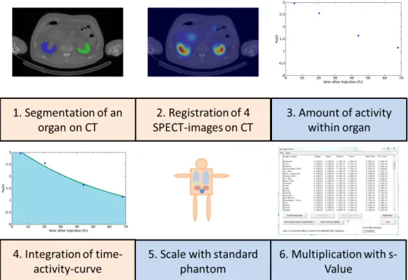
Figure 1.1: Steps of the dosimetry chain according to the MIRD protocol – Multiplication of a global dose kernel, called S-value, with the cumu-

lated activity according to MIRD

– Convolution of activity distributions with dose-voxel-kernels (DVK) – Full Monte Carlo simulation (MC)

Any successful implementation has to rely on a close collaboration of medical physicists and technologists.

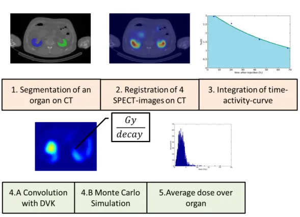
The order of the steps can vary, depending on the used dose calculation method.

In figure 1.1 the steps for the MIRD-method are illustrated. For the voxel-wise methods (MC and DVK), three steps are identical but are applied in a different order as can be seen in figure 1.2.

The three dose estimation methods require the assessment of the 3D distribu-

tion of the radionuclide within the body. Over the last few years, efforts moved

towards image processing methods to quantify a spatial and temporal activity dis-

tribution with good accuracy [48], [90], [27], [26]. With the advent of the latest

PET/CT and SPECT/CT technologies, quantification of activity distributions can

be performed with resolutions adequate for voxel dosimetry, typically of 5 mm

or even less, co-registering functional and anatomical images. The information of

both

(21)

1.2. THE DOSIMETRY CHAIN FOR RADIONUCLIDE THERAPY 21

Figure 1.2: Steps of a voxel-wise dosimetry chain

• density pattern (Computed Tomograpy (CT)) and

• accumulated activity distribution (SPECT),

available in a voxel geometry, form essential resources for any dose estimation.

If SPECT images are available at subsequent time points, the time dependence of the activity distribution, the (Time Activity Curve (TAC)), can be modeled. In this study, the number of decays, i. e. the integral over the TAC, has been estimated from 4 SPECT images and one CT image.

X-ray CT provides depth information from multiple projections. Image recon-

struction from multiple projections assumes that the activity distribution remains

stationary throughout the acquisition. This means that the difference in spatial

distribution of nuclear disintegrations is, in the acquired projection images, only

a function of the projection view. The task for any reconstruction method is then

to estimate the individual activity distribution in the patient, possibly at a number

of subsequent time points. For many years, Filtered Back-Projection (FBP) was

the golden standard of reconstruction methods, but today, the clinical use of itera-

tive reconstruction methods is established. This family of reconstruction methods

all include a computer model of the imaging system. The principal steps in an

iterative reconstruction method are the following:

(22)

• From a first estimate of the internal source distribution, the computer model calculates a projection image.

• This image is then compared with a measured projection to determine where in the modeled image differences occur.

• Most reconstructions in nuclear medicine use the Expectation Maximization (EM) algorithm [34], [101], [79].

Iterations go on until the ratio between the modeled and the measured data converges to one. The initial image is multiplied by a tomographic error image.

The latter is obtained from back-projecting the ratios. This is done for all projec- tion angles. Note that the noise in these images shows a Poisson distribution. A version of the EM algorithm is the ordered-subsets EM algorithm [63].

1.2.1 Time-Activity-Curve (TAC)

The amount and rates of radiopharmaceutical uptake and excretion is governed by passive as well as active physiological mechanisms and varies amongst individu- als. These parameters directly influence absorbed dose calculations and need to be determined for each patient. The method used to determine TACs for different organs and tissues is

• to perform imaging at several time points after radiopharmaceutical admin- istration and

• to determine the activity concentration in different tissues at every time point.

The absorbed dose is associated with the area under this TAC. The activity A(t) of a radionuclide is given as the number of nuclear disintegrations N (t) per unit time and decreases exponentially in time. Thus a sum of exponential curves with different time constants can then be used to fit patient data [148] according to

A(t) = X

S∈S

A(r

_S

, 0) exp(−λ

_phys

· t)

where A(t) = dN (t)/dt denotes the total activity, A(r

S

, t) = dN (r

S

, t)/dt the

nuclide-specific activity at voxel location r

_S

in the Volume Of Interest (VOI) S

and where the rate constant λ

_phys

= 1/(τ

_phys

) describes the kinetics of removal

of activity components A(r

S

, t) with a nuclide-specific lifetime τ

phys

. The latter

is related to the half-time of the nuclide via t

_1/2

= ln(2)τ. In addition to this

(23)

1.2. THE DOSIMETRY CHAIN FOR RADIONUCLIDE THERAPY 23 physical lifetime, also a biological lifetime is of relevance for removing activity components. If the biological removal also follows an exponential law, the rate constants can be summed up to an effective rate constant

λ

_{ef f}

= λ

_phy

+ λ

_biol

(1.1)

which results in an effective lifetime

τ

_{ef f}

= τ

_biol

· τ

_phys

τ

biol

+ τ

phys

(1.2) This finally results in a Time Integrated Activity (TIA) given by

A(r ˜

_S

) ≡ N(r

_S

) = Z

∞

0

A(t)dt = X

i

Z

∞ 0

A(r

_S

, 0)e

^−λ^{ef f}^(r^S^)·t

dt

= X

S

A(r

_S

, 0)

λ

ef f

(r

S

) = X

S

·A(r

_S

, 0) · τ

_{ef f}

(r

_S

) (1.3) where the sum extends over all voxels of the entire VOI. Note that for the effective lifetime we have

τ

_{ef f}

≤

τ

_phys

if τ

_phys

≤ τ

_biol

τ

biol

if τ

biol

< τ

phys

(1.4) Note also that solving the equation for an effective lifetime, the units for the bi- ological and physical lifetimes must be the same. If a voxel-wise dosimetry is performed, the integration of the time activity curve results in a voxel-wise map of the number of decays per voxel. For the MIRD method, the number of decays, which take place in the kidney, can be calculated by integration.

1.2.2 Energy dose rate and energy dose

The rate dD

_E

(r

_T

, t)/dt at which, at time t after administration, radiation energy dose is delivered within a patient to target tissue at location r

_T

from a radioactive material distributed uniformly within source tissue located at r

S

is given as:

dD

_E

(r

_T

, t)

dt := ˙ D

_E

(r

_T

, t) = A(r

_S

, t)K(r

_T

← r

_S

, t) J

kg · s = Gy s

(1.5)

where A(r

_S

, t) is the time-dependent activity of a radionuclide in source tissue r

_S

,

i.e. A(r

S

, t) counts the number of nuclear disintegrations happening at time t in

source tissue located at r

_S

. Further, K (r

_T

← r

_S

, t) = ˙ D

_E

(r

_T

, t)/A(r

_S

, t) denotes

(24)

the radionuclide-specific energy dose kernel representing, at time t after admin- istration, the energy dose absorbed in target tissue r

_T

per unit activity present in source tissue r

_S

. The energy dose rate, i. e. d

²

E(r

_T

, t)/dm dt = dD

_E

/dt, thus denotes how much energy is deposited in a unit mass in unit time. In practice, more handy units are

^µGy_hr

or

^mGy_yr

.

Absorbed energy dose D

_E

(r

_T

), i. e. the deposited radiation energy per unit mass over a timespan T

_D

, is the fundamental quantity for coupling to the radiobi- ological effect. It is defined as the radiation energy dE(r

_T

) absorbed in a target tissue contained in a volume dV

_T

= d

³

r

_T

with mass density ρ

_m

yielding a target mass dm = ρ

_m

d

³

r

_T

, i. e. we have

D

_E

(r

_T

) := dE(r

_T

) dm

= dE(r

_T

)

ρ

_m

dV

_T

= (r

_T

) ρ

_m

=

Z

TD

0

dD

_E

(r

_T

, t) dt dt

= X

rS

Z

TD

0

A(r

_S

, t)K(r

_T

← r

_S

, t)dt

≈ X

r_S

A(r ˜

_S

)K (r

_T

← r

_S

) (1.6)

measured in h

J

kg

≡ Gy i

. The time-dependent activity in the source tissue A(r

_S

, t) is obtained

• by numeric solution of a set of first-order coupled differential equations de- fined by compartment models for all organs and suborgan tissues of interest.

• directly via quantitative imaging, including planar imaging, SPECT, and Positron-Emission Tomography (PET), or by tissue sampling (e.g., biopsy, blood, or urine collection).

In most instances, the time dependence of the dose kernel K(r

T

← r

S

, t) may be neglected, as when the source and target masses remain constant over the period of irradiation, justifying the use of the approximation given with the last equation. The integral

A(r ˜

_S

) = Z

t2

t1

A(r

_s

, t)dt (1.7)

(25)

1.2. THE DOSIMETRY CHAIN FOR RADIONUCLIDE THERAPY 25 is usually called time-integrated or cumulated activity (TIA) and describes the total number of decays occurring in the source region during the time interval T

_D

. In nuclear medicine, due to tissue heterogeneities, mean absorbed energy dose hD

_E

(r

_T

)i is quoted, which is given by

hD

_E

(r

_T

)i = 1 M

_T

Z

VT

D

_E

(r)ρ

_m

(r)d

³

r (1.8) where M

_T

is the total mass of tissue inside a target volume V

_T

. The latter might represent a tissue voxel or a whole organ for which the absorbed dose is deter- mined.

In order to account for the biological effect of the radiation, equivalent energy dose D

_eq

= w ·D

_E

[Sv] has to be considered, where Sv denotes Sievert and w rep- resents a tissue-related weight factor (often called relative biological efficiency).

The weights are w = 1 for electrons and photons, but w = 20 for α - particles and w = 2 − 20 for neutrons depending on their kinetic energy.

If the fluency Ψ of a particle beam is known, the energy dose can be computed as

D

_E

= N dE

dm = N dE

ρ

_m

dV = 1 ρ

_m

N σ

dE dx D

_E

· ρ

_m

= Ψ · LET

where N is the number of particles, σ the beam cross section, Ψ = N/σ is the fluency, ρ

_m

the mass density and dE/dx the energy loss per unit length, also called stopping power or linear energy transfer.

Energy dose should not be confused with radiation dose D

_Q

, which denotes the amount of charge dQ [C] deposited in a unit mass dm [kg]. Accordingly we have

D

_Q

= dQ dm

C kg

1.2.3 Radiation energy transport and dose kernels

In Radiotherapy, any dosimetry of internally distributed radionuclides relies on the description of the radiation energy transport from a source to a target region [160], i. e.

hD

_E

(r

_T

)i = X

rS

A(r ˜

_S

) · K(r

_T

← r

_S

)

Here the dose kernel is given by

(26)

K (r

_T

← r

_S

) = c M

_T

X

i

n

_i

E

_i

Φ (r

_T

← r

_S

, E

_i

)

where c = 1 [(Gy·kg)/(M Bq·s·M eV )] if D

E

[Gy], A ˜ [M Bq·s], E

i

[M eV ], m [kg], and c = 2.13 if D

_E

[rad], A [µCi], m [g], E

_i

[M eV ] [94]. The dose kernel K(r

_T

← r

_S

), if summed up over all fractions of absorbed energy Φ(r

_T

← r

_S

, E

_i

) within a whole organ, is commonly called S-value. It is measured in [Gy/(Bq ·s]).

Here the absorbed fraction Φ (r

_T

← r

_S

, E

_i

) of incident radiation energy repre- sents the ratio of the energy E absorbed in target region r

_T

to the energy E

₀

emitted in the source region r

S

Φ(r

_T

← r

_S

) = E(r

_T

) E

₀

(r

_S

)

Furthermore, specific absorbed fraction Φ

_spec

of energy is the ratio of absorbed fraction by the mass of the target tissue m

_T

Φ

_spec

(r

_T

← r

_S

) = Φ(r

_T

← r

_S

) m

_T

Thus the S-value represents the mean absorbed dose hD

_E

(r

_T

)i to the target organ centered at location r

_T

per unit of accumulated activity A(r ˜

_S

) in the source region r

_S

, that is to say, it describes the fraction of the kinetic energy E

_kin

[J ] released by each particle type, i, with n

_i

emitted particles per radioactive decay, which will be absorbed in the target volume with total mass M

_T

(t) [kg]. Hereby

∆

_i

= n

_i

E

_i

, where E

_i

represents the energy emitted for radiation type i with prob- ability n

_i

. In principle, the equation is valid for different kinds of volumes, from organs down to cells, but for smaller volumes, the stochastic nature of radiation interaction renders the mean value less representative of the actual energy deposi- tion.

1.2.4 MIRD-method

The method defines a protocol for an estimation of the absorbed energy dose to organs of interest using anatomic phantoms representative of any patient or, at least, an average patient. This method computes the mean organ dose due to

• electron and α-particle emissions with their accompanying photon emis- sions within the source organ, and

• the energy dose deposited by photons emitted within surrounding organs

and tissues.

(27)

1.2. THE DOSIMETRY CHAIN FOR RADIONUCLIDE THERAPY 27 This technique represents a macroscopic approach to dose estimation and is currently implemented in the Organ Level Internal Dose Assessment with Expo- nential Modeling (OLINDA) software [149]. The method is easy to use, but only an average absorbed dose hD

_E

i can be estimated. Neither heterogeneities in ei- ther tissue composition or radioactivity distribution nor the anatomic geometry of the source and target tissues within the body of the patient are considered.

Dosimetric parameters relevant to the MIRD protocol

In any real internal dose problem, there will be more than one organ which con- centrates the activity, and many targets for which the absorbed dose is required.

In this case, the MIRD equation needs to be solved for each source region r

S

and target region r

_T

as follows [150].:

D

_E

(r

_T

) = X

S

A(r ˜

_S

)S(r

_T

← r

_S

)

= A

₀

X

S

τ

_S

S(r

_T

← r

_S

)

= c

M

_T

X

S

w

S

A(r ˜

S

) X

i

n

i

E

i

Φ

i

(r

T

← r

S

) where a source residence time τ

_S

is defined as

τ

S

=

A(r ˜

_S

) A

₀

and where A

₀

is the administered activity. Thus more than one organ can be taken into consideration using compartmental modeling [107]. Goodness of fit can be assessed through an Akaike information criterion (AIC) [81] or an F-test [89].

Attempts have also been made to compile patient data in order to use the group behavior as a prior when applying Bayesian techniques.

These generic expressions comply well with the most recent MIRD expres- sions discussed above. The OLINDA software uses a somewhat simpler expres- sion given by

D = N · DF DF = k

m X

i

n

_i

E

_i

Φ

_i

w

_r_i

where DF is conceptually similar to the S-value defined in the MIRD system.

The number N ≡ A(r ˜

_S

) of disintegrations is the integral of a time-activity curve

(28)

for a source region. A number of anthropomorphic phantoms exist that can be used to produce dose estimates for standardized individuals.

1.2.5 Voxelwise dosimetry

Voxelwise dosimetry represents a mesoscopic approach to dose estimation. It means employing voxelized geometries in representing organs as tagged voxels of differing activity levels. MC radiation transport simulations then assess dose at the voxel level. Geometries have to be deduced from phantoms or from a regional CT image of the patient [144], [171]. The MC approach, furthermore, can yield a Dose Voxel Histogram for radiation sources both inside and outside the target organ.

The average energy dose hD

_E

i absorbed at any target organ can be obtained by tracking energy deposition events within the target organ by direct MC transport simulations. The computations consider two contributions:

• The average absorbed dose to a voxel within the organ of interest due to α- and β-particle as well as γ-photon emissions within that organ

• The energy dose to a voxel in the organ of interest due to γ -photon emissions in the surrounding organs or tissues.

The technique can handle tissue heterogeneities (bone, soft tissue, air, lung, and such) as well as patient-specific anatomic geometry of all source and target tissues as well as the non-uniform source distributions [61], [60], [35], [123].

Because of statistical sampling limitations, the energy dose is usually averaged across a group of voxels or all voxels of a given target organ. However, the ap- proach is time-consuming and computationally demanding. For anatomic regions characterized by a uniform tissue density, the S-value technique represents an ex- cellent option, with rapid computation and still-good dosimetric accuracy [36]. In particular, the S-value concept is possibly the most applied, easy to implement, not requiring volume and complying with the familiar MIRD formalism [84]. But the S-value method represents a macroscopic approach lacking resolution at the voxel level. With it, dose values can only be calculated for whole organs.

If one is to boil down the resolution to the size of single voxels, currently two different methods exist for performing internal dosimetry at the voxel level [157], [152]:

• the above mentioned full Monte Carlo simulation (MC) or

• a convolution with a dose-voxel-kernel (DVK).

(29)

1.2. THE DOSIMETRY CHAIN FOR RADIONUCLIDE THERAPY 29 When the amount and distribution of radioactivity A(r

_T

, t), represented in the SPECT- or PET-image is known, the resulting energy dose distribution D

_E

(r

_T

, t) can be determined by transforming the activity distribution from the image to absorbed radiation energy using an appropriate dose kernel K(r

_T

← r

_S

). The source and target regions centered at r

_S

and r

_T

, respectively, are those defined within the anatomic model and may represent voxels from SPECT or PET images.

Hence, r

S

denotes the location of the source voxel and r

T

the corresponding loca- tion of the target voxel. The kernel thus contains information on how the radiation energy resulting from one nuclear disintegration is spatially deposited. The kernel transfers an activity distribution to an absorbed energy distribution by weighting the energy deposition of the particles over its range. An energy deposition im- age is obtained by applying the kernel to the original activity distribution image through a convolutive filtering process. Each voxel assigns energy, measured in either [J] or [M eV ], and by dividing it with the mass of the voxel, a specific en- ergy, or absorbed dose, measured in [Gy ] can be generated in each voxel of the image. The values in this specific energy (or dose) image can then be used to generate a Dose-Volume Histogram [40]. The latter presents the volume (or a per- centage of the volume) that receives some dose in a given range of dose levels. If the respective volume refers to one voxel, this is referred to as DVK dosimetry.

The DVK method is widely used today, particularly for the more commonly used radionuclides which emit electrons, including Auger electrons, and photons.

In summary, at the voxel level, the absorbed dose to a target voxel located at r

_T

due to the cumulated activities in source voxels located at r

_S

can be expressed as:

D

_E

(r

_T

) = X

S∈S

A(r ˜

_S

)K

_vox

(r

_T

← r

_S

)

where the sum is extended to all source voxels. In voxel-wise dosimetry, the DVK

is defined as the absorbed dose to the target voxel per unit decay in the source

voxel, when both voxels are contained in an infinite homogeneous medium of

mass density ρ

_m

. According to this definition, DVKs can be obtained by MC

simulations of voxel geometries representing an infinite medium of uniform com-

position. The radionuclide is placed at the center of this geometry, and the ab-

sorbed dose is scored in surrounding voxels. The mathematical convolution of

pre-calculated DVKs, i. e. energy dose per unit decay as a function of distance,

with a cumulated activity map provides the absorbed dose distribution for the bi-

ological system considered [98].

(30)

1.3 Uncertainties in dose estimation

Any error analysis has to start with the data collection systems. Data uncertainty my result from limitations on energy resolution, low spatial resolution due to col- limator septal penetration by high energy photons, data loss due to scatter and attenuation as well as inherent statistical variations of measurements on radionu- clides. Reports on total error quantifications range from a few percent for large organs to some 20 % for small or low Signal to Noise Ratio (SNR) objects. A summary of the terms contributing to uncertainties in calculated dose estimates in nuclear medicine was given by [150] in terms of the variability of the nuclear medicine population. The conclusion was that the two variables with highest im- pact onto error estimates were the cumulated activity A ˜ and organ masses m.

Further issues to be considered are the following:

• The biokinetic parameters, fractional uptake and half-life, vary substantially (factor > 2) across individuals. So, just applying a dose coefficient, mea- sured in [mSv/M Bq], from a standard model to any given patient leads to a relatively large uncertainty in dose estimation [106]. It is unfortunate that patient-individualized dose calculations are not performed routinely for therapeutic administrations of radiopharmaceuticals, although this practice is increasing in Europe [44], [11], [19], [117].

• Simply administering a standard activity ( A ˜ [M Bq]) or specific activity

( A/M ˜ [M Bq/kg], A/O ˜ [M Bq/m

²

]) per unit body mass M or surface area

O to all patients cannot permit the delivery of an adequate therapy to all

patients. In general, several nuclear medicine images are needed, yielding

A(r

_S

, t) to establish the uptake and clearance patterns in normal tissues and

tumors [147].

(31)

Chapter 2 Monte Carlo Simulation (MC)

The following short summary lends credit from [75].

Photons interact with surrounding matter via four basic processes:

• Rayleigh scattering: A coherent scattering with the molecules (or atoms) of the medium

• Photoeffect: A photo-electric absorption of a photon and transfer of its en- ergy to an electron

• Compton scattering: An incoherent scattering with atomic electrons

• Particle production: A materialization into an electron/positron pair in the electromagnetic field of the nuclei and surrounding atomic electrons The last three collision types transfer energy from the photon beam to elec- trons. Depending on energy and the medium, in which the transport takes place, one of them dominates the total absorption cross-section:

• At low energies, E < 100 keV , the Photoeffect dominates .

• At intermediate energies, 100 keV ≤ E ≤ 1 M eV , the Compton effect is the most important process .

• The pair production process dominates at energies E ≥ 1.02 M eV larger than the mass - equivalent energy of the resting particle pair.

Electrons, as they traverse matter, loose energy by three basic processes:

• Inelastic collisions with atomic electrons

• Bremsstrahlung and positron annihilation

31

(32)

Radiative energy loss transfers energy back to photons and leads to the cou- pling of the electron and photon radiation fields. The bremsstrahlung process is the dominant mechanism of electron energy loss at high energies, inelastic col- lisions are more important at low energies. In addition, electrons participate in elastic collisions with atomic nuclei which occur at a high rate and lead to fre- quent changes in the electron direction. Inelastic electron collisions and photon interactions with atomic electrons lead to excitations and ionizations of the atoms along the paths of the particles. Highly excited atoms, with vacancies in inner shells, relax via the emission of photons and electrons with characteristic ener- gies.

The coupled integro-differential equations that describe the electromagnetic shower development are prohibitively complicated to allow for an analytical treat- ment except under severe approximations. The MC technique is the only known solution method that can be applied for any energy range of interest. MC of parti- cle transport processes are a faithful simulation of physical reality:

• Particles are drawn from a source distribution deduced from activity distri- butions known across a target VOI

• These particles travel certain distances, determined by a probability distri- bution depending on the total interaction cross section Ω

• At the site of a collision, they scatter into another energy and/or direction according to the corresponding differential cross section σ

• During such collisions, possibly new particles are produced that have to be transported as well.

This procedure is continued until all particles are absorbed or leave the VOI under consideration.

Quantities of interest can be calculated by averaging over a given set of MC particle histories (also refereed to as showers or cases). From mathematical points of view each particle history is one point in a d-dimensional space (the dimension- ality depends on the number of interactions) and the averaging procedure corre- sponds to a d-dimensional MC integration. As such, the MC estimate of quantities of interest is subject to a statistical uncertainty which depends on N , the number of particle histories simulated, and usually decreases as N

^−1/2

. Depending on the problem under investigation and the desired statistical accuracy, very long calcu- lation times may be necessary.

An additional difficulty occurs in the case of the MC of electron transport. In

the process of slowing down, a typical fast electron and the secondary particles

it creates undergo hundreds of thousands of interactions with surrounding matter.

(33)

2.1. RADIONUCLIDE 33 Because of this large number of collisions, an event-by-event simulation of elec- tron transport is often not possible due to limitations in computing power. To cir- cumvent this difficulty, Berger [14] developed the “condensed history” technique for the simulation of charged particle transport. In this method, large numbers of subsequent transport and collision processes are “condensed” to a single “step”.

The cumulative effect of the individual interactions is taken into account by sam- pling the change of the particle’s energy, direction of motion, and position, at the end of the step from appropriate multiple scattering distributions. The condensed history technique was motivated by the fact that single collisions with the atoms cause in most cases only minor changes in the particle’s energy and direction of flight. This technique made MC of a charged particle transport possible but intro- duced an artificial parameter, the step-length. The dependence of the calculated result on the step-length has become known as a step-size artifact [17].

2.1 Radionuclide

For estimating the absorbed radiation dose elicited from a

¹⁷⁷

Lu radiation source into the surrounding tissue (air, lung, bone), N MC have been performed, each encompassing M nuclear disintegrations, shortly called radioactive decays.

During one such decay,

¹⁷⁷

Lu transforms into

¹⁷⁷

Hf according to the follow- ing state transitions.

The related γ - radiation shows several spectral lines according to the scheme

seen above and the lines exhibit very small line widths. Hence, one could model

the spectrum as a sum of discrete Lorentzians.

(34)

Here a Lorentzian line is given in the time domain and its conjugated Fourier domain, respectively by

L(t) = H(t)L

₀

exp(−t/τ ) L(ω) = L

₀

1/τ + iω = L

₀

p (1/τ )

²

+ ω

²

exp(−iφ)

where H(t) denotes the Heaviside step function, ω = 2πν with ν [Hz] the fre- quency, τ the average life-time, φ = arctan(ωτ ) and i = √

−1 denotes Euler’s number. The Lorentzian line in the frequency domain consist of a real and an imaginary part according to

L(ω) = (1/τ )L

0

(1/τ )

²

+ ω

²

− i ωL

0

(1/τ )

²

+ ω

²

= τ L

₀

1 1 + (ωτ )

²

− i ωτ 1 + (ωτ )

²

The real part of this complex Lorentzian provides the conventionally observed absorption mode, often called a Lorentz line.

Hence, using

¹⁷⁷

Lu the main dates are:

Table 2.1: Relevant characteristic quantities of a

¹⁷⁷

Lu radiation Nuclide β(M eV ) Range (mm) T

_1/2

(d) γ(keV )

177

Lu 0, 50 2 6, 7 113(6%)

2.2 Standard Error for Dose Estimation

In the following, the dose will be denoted by X and is considered a random vari- able resulting from independent nuclear disintegrations, simply called decays.

Hence, x

_mn

denotes the decay event m happening in simulation run n inside a voxel of volume V

_vox

[mm

³

] = 4.7 [mm] · 4.7 [mm] · 4.7 [mm] and tissue density ρ

_m

[mg · mm

⁻³

] where m denotes the average mass of either air, lung tissue or bone.

Following, we will consider two strategies:

• Consider M simulated decays as one sample of data and simulate N such

samples in total

(35)

2.2. STANDARD ERROR FOR DOSE ESTIMATION 35

• Consider N M simulated decays as one grand sample of data and simulate L such grand samples in total

Typically we talk about N ≈ 10

²

and M ≈ 10

⁴

.

Relation between standard error (SE) and standard deviation (SD) The Stan- dard Error (SE) denotes the Standard Deviation (SD) of a sampling distribution of a statistic. The latter can be, for example, the average energy dose hD

E

(r

T

)i

Vvox

in a voxel of tissue. Hence, the SE depicts the dispersion of sample means around the population mean, while the SD denotes the dispersion of individual measure- ments around the population mean.

Now for a given sample size, the SE equals the SD divided by the square root of the Sample Size (SS), i. e.

SE = SD

√ SS

Following we denote the sample SE by se

_n

and the grand SE by SE, the sample SD by sd

_n

and the grand SD by SD.

Sample SE First we consider each

¹⁷⁷

Lu decay as an independent event and we simulate M such decays. We then consider these M simulated decays as one sample of data. Each such decay deposits an amount x

_mn

[Gy] of energy dose in the surrounding tissue. Averaging over M independent decay events yields an average energy dose

hx

_n

i = 1 M

M

X

m=1

x

_mn

which we call sample mean and which is deposited in one voxel during one single simulation run n. The size of the sample is now SS = M . Each single dose x

_nm

, deposited in one voxel during one decay event, is scattered around its sample mean hx

_n

i, and this scatter is characterized by the corrected sample standard deviation

sd

_n

= v u u t

1 M − 1

M

X

m=1

(x

_mn

− hx

_n

i)

²

where the factor in front of the sum term represents the Bessel correction (M − 1

instead of M ), which assures an unbiased variance (not standard deviation! The

latter is still biased due to the non-linear sqrt operation). The sample standard

deviation then yields a sample standard error according to

(36)

se

n

= sd

n

√ M

= 1

√ M

v u u t

1 M − 1

M

X

m=1

(x

_mn

− hx

_n

i)

²

≈ 1 M

v u u t

M

X

m=1

(x

_mn

− hx

_n

i)

²

≈ 1 M

v u u t

M

X

m=1

x

²_mn

− M hx

_n

i

²

(2.1)

Repeating such simulations N times, yields N samples of mean energy doses deposited in a voxel. These N samples provide an estimate of the underlying un- known sampling distribution of mean energy doses hx

_n

i deposited in each voxel.

The underlying sampling distribution can be characterized by

• a grand average deposited energy dose which, in abuse of notation, could be called a population mean

hhxii = 1 N

N

X

n=1

hx

_n

i = 1 M N

N

X

n=1 M

X

m=1

x

_mn

Note that if N → ∞, then the grand average tends towards the population mean energy dose.

• the grand mean standard deviation of the fluctuating sample means around the grand average, i. e. the width of the sampling distribution, which we could accordingly call the standard deviation of the mean

SD = v u u t

1 N − 1

N

X

n=1

(hx

_n

i

_M

− hhxii

_{M N}

)

²

= v u u t

1 N − 1

"

_N

X

n=1

hx

n

i

²_M

− N hhxii

²_{M N}

Estimation of Dose Distribution for Lu-177 Therapies in Nuclear Medicine