Improved calculation of offshore meteorological parameters for applications in wind energy

offshore

meteorological parameters for applications in

wind energy

Inaugural-Dissertation

zur

Erlangung des Doktorgrades

der Mathematisch-Naturwissenschaftlichen Fakult¨ at der Universit¨ at zu K¨ oln

vorgelegt von

Richard J. Foreman aus Adelaide

K¨ oln

im Januar 2012

Berichterstatter: Prof. Dr. Stefan Emeis Prof. Dr. Michael Kerschgens

Tag der m¨ undlichen Pr¨ ufung: 03.04.2012

Work presented in this thesis demonstrates an improved calculation of offshore meteorological parameters, in particular the wind speed and turbulence inten- sity, relevant for wind energy applications. An alternative offshore drag law is proposed that anticipates drag coefficients at intermediate wind speeds expected in applications for wind energy, but is also consistent with the functional be- haviour of drag coefficients as a function of wind speed expected at tropical cyclone wind speeds. The law is compared with measurements recorded at the FINO1 platform in the North Sea and with those reported in the literature, where differences are attributed to the nature of the water wave field. A cor- relation equation connecting the air side drag coefficients and water side wave steepnesses is then proposed which can also anticipate drag coefficients expected at tropical cyclone wind speeds using measurements from a buoy recorded dur- ing hurricane Rita (2005). The correlation equation interpolates between two hypothesised asymptotic regimes: One whereby drag coefficients scale with the squared wave steepness and the other whereby drag coefficients are constant. At wind speeds relevant for wind energy purposes, two distinctive wave steepness scaling regimes were detected in measurements recorded at FINO1, which are also evident in results reported in the literature. A higher order correlation at- tempted here, but left open for further development in the future, finds that the unsteady orientation of the wind with the wave direction is likely a further im- portant parameter. This is found by analysing a stable internal boundary layer detected at FINO1 for a period of about a week, which resulted in a diurnal cycle of offshore meteorological parameters including the wind direction. An os- cillation was correspondingly found in buoy measurements of wave steepnesses during this period, and hence in drag coefficients. It is demonstrated if higher order wave field effects can be correctly accounted for, an enhanced calculation in the wind speed will result.

The nature of the stable internal boundary layer then facilitated investiga- tion throughout a large portion of the boundary layer by the 100 m high FINO1 tower, due to the relatively shallow (O(100) m) height of the internal layer. Com- parison with numerical simulations using the Mellor-Yamada-Janji´ c planetary boundary layer parametrization within the Weather Research and Forecasting model showed contrasting vertical profiles of turbulent kinetic energy compared with the measurements. This consequently resulted in an overprediction of tur- bulence intensities as calculated by the model compared with FINO1 measure- ments at 80 m above the sea surface, and an underprediction of turbulence closer to the surface as inferred from previously reported work in the literature. It is shown here that an improved calculation of turbulence is possible by making changes to the selection of the closure constants and the surface length scale.

3

Die vorliegende Doktorarbeit pr¨ asentiert eine verbesserte Berechnung meteorol- ogischer Parameter in der marinen atmosph¨ arischen Grenzschicht, insbesondere der Windgeschwindigkeit und der Turbulenzintensit¨ at, geeignet f¨ ur Winden- ergieanwendungen. Es wird ein alternatives Widerstandsgesetz vorgeschla- gen, das den Luftwiderstandsbeiwert bei mittleren Windgeschwindigkeiten gut widergibt, und das auch dem praktischen Verh¨ altnis zwischen dem Widerstands- beiwert und der Windgeschwindigkeit bei tropischen Wirbelst¨ urmen entspricht.

Das Gesetz wird mit Messungen der FINO1 Messplattform in der Nordsee und vorhandenen Messungen in der Literatur verglichen. Die gefundenen Un- terschiede in den Messungen werden dem Charakter des Wasser-Wellenfelds zugeschrieben.

Es wird eine Korrelationsgleichung vorgeschlagen, die den Luftwiderstands- beiwert und die Wellensteilheit verbindet und die erwarteten Luftwiderstands- beiwerte w¨ ahrend Wirbelsturms Rita (2005) berechnen kann. Die Korrelations- gleichung interpoliert zwischen zwei vorausgesetzten asymptotischen Regimen:

In einem Regime entspricht der Luftwiderstandsbeiwert dem Quadrat der Wellensteilheit und im anderen ist der Luftwiderstandsbeiwert konstant. Bei Windgeschwindigkeiten, die f¨ ur Windenergieerzeugung relevant sind, werden zwei charakteristische Wellensteilheitsregime in den Messungen von FINO1 ent- deckt. Die gleichen Ergebnisse werden auch in der Literatur nachgewiesen.

Eine Korrelation h¨ oherer Ordnung zwischen Wind und Wellen wird eben- falls untersucht, mit dem Ergebnis, dass auch die variable Orientierung der Windrichtung wichtig ist. Dieses Ergebnis wird bei einer Analyse einer Episode mit einer sehr stabilen Grenzschicht in den FINO1-Messungen gefunden, die eine Woche andauerte und einen deutlichen Tagesgang aufwies, einschließlich der Windrichtung. Entsprechend wurde in diesem Zeitraum auch bei den Bojen- Messungen zur Wellensteilheit eine Oszillation festgestellt, und demzufolge auch im Luftwiderstandsbeiwert. Es wird dargestellt, dass eine Ber¨ ucksichtigung des Wind-Wellen Parameters h¨ oherer Ordnung, eine verbesserte Berechnung der Windgeschwindigkeit erm¨ oglichen wird. Die weitere Auswertung und Entwick- lung bleibt zuk¨ unftiger Forschung ¨ uberlassen.

Weiterhin erlaubt die geringe H¨ ohe der sehr stabilen Grenzschicht eine Un- tersuchung eines großen, vertikalen Teils dieser Grenzschicht aus den FINO1- Daten bis 100 m H¨ ohe. Werden die gemessenen vertikalen Profile der turbu- lenten kinetischen Energie mit Ergebnissen der Grenzschichtparameterisierung von Mellor-Yamada-Janji´ c in numerischen Modellen wie dem Weather Research und Forecasting (WRF) Modell verglichen, zeigt sich ein deutlicher Unterschied zwischen Messungen und Modellen. Dies resultiert f¨ ur die sehr stabile Schich- tung in vom Modell zu hoch berechneten Turbulenzintensit¨ aten in 80 m H¨ ohe,

5

Bei weniger stabilen Grenzschichten wird festgestellt, dass die vorgeschlage-

nen Ver¨ anderungen in der Turbulenzparametrisierung auch hier eine verbesserte

Berechnung der Turbulenzintensit¨ at erm¨ oglichen.

The following thesis originally arose from the idea of my supervisor Prof. Dr.

Stefan Emeis concerning the possibility that there may be something unique about the nature of offshore turbulence to be subsequently included in numer- ical weather prediction models. I thus would like to thank Prof. Dr. Emeis for accepting me as his PhD student here at the Institute for Meteorology and Cli- mate Research (IMK-IFU), Garmisch-Partenkirchen and providing much sup- port and advice the last three years. I hope that the following thesis has gone some way to answering his question and is also useful for others wanting to further pursue work in this fascinating field.

In addition to Prof. Dr. Emeis, I would also like to thank the many people here at the IMK-IFU whose help I have received in some manner which has enabled this work to be carried out. In particular, I would like to mention the efforts of Drs. Johannes Werhahn and Peter Suppan.

The work in this thesis follows from the thesis of Dr. Matthias T¨ urk, whom I thank for making his processed data available for use here. The original data comes courtesy of the German wind energy insitute (DEWI) and the German maritime and hydrographic agency (BSH) which are also gratefully acknowl- edged. This thesis was done within the VERITAS project (work package 5 of OWEA) which is funded by the German Ministry of the Environment (BMU) via the PTJ (FKZ 0325060).

Many thanks to der Mathematisch-Naturwissenschaftlichen Fakult¨ at der Universit¨ at zu K¨ oln, in particular Prof. Dr. Michael Kerschgens, for giving me the opportunity to obtain my PhD from their institute whilst working from afar here in Garmisch-Partenkirchen.

On a personal note, I am deeply thankful for all the support I have received from Indra Lopez both leading up to and during this thesis. Back home, I would like to thank David and Martyn Foreman, as well as Dr. Zebb Prime for their long distance support.

7

Abstract 3

Zusammenfassung 5

Acknowledgments 7

Notation 11

List of Figures 14

List of Tables 23

1 Introduction 25

1.1 Introduction . . . . 25

1.2 Problem Definition . . . . 27

1.3 Methodology . . . . 30

1.4 Scope . . . . 31

2 Offshore surface roughness effects 35 2.1 Introduction . . . . 35

2.2 Surface roughness . . . . 36

2.2.1 Offshore roughness . . . . 36

2.2.2 Drag coefficient . . . . 38

2.2.3 Stratification effects . . . . 39

2.2.4 Froude number effects . . . . 41

2.3 FINO1 . . . . 42

2.3.1 Data Description . . . . 42

2.3.2 January 2005 . . . . 43

2.3.3 February 2005 . . . . 48

2.3.4 November 2005 . . . . 54

2.4 Tropical cyclone wind speeds . . . . 58

2.5 Conclusion . . . . 59

3 Offshore aspect ratio effects 61 3.1 Introduction . . . . 61

3.2 Scaling Analysis . . . . 62

3.2.1 Introduction . . . . 62

3.2.2 Toba’s

power law . . . . 64

3.2.3 Extension of Toba’s

power law . . . . 65

9

3.3.2 Literature . . . . 73

3.3.3 Tropical Cyclones . . . . 78

3.4 Conclusions . . . . 80

4 Air/Sea/Land interaction effects 83 4.1 Introduction . . . . 83

4.2 Results from previous analyses . . . . 85

4.3 General description of WRF and the Mellor-Yamada-Janji´ c Model 87 4.4 Results . . . . 89

4.4.1 Mean fields . . . . 89

4.4.2 Turbulent fields . . . . 95

4.4.3 Model results . . . . 99

4.5 Conclusions . . . 107

5 Mellor-Yamada-Janji´ c model modifications 109 5.1 Introduction . . . 109

5.2 Description of the MYJ model . . . 110

5.3 Determination of the closure constants . . . 114

5.3.1 Traditional approach . . . 114

5.3.2 Alternative strategy to the traditional approach . . . 116

5.4 Single Column Model Results . . . 124

5.5 Conclusions . . . 128

6 Applications for wind energy 131 6.1 Introduction . . . 131

6.2 Results . . . 134

6.2.1 May 2006 . . . 134

6.2.2 January 2005 . . . 141

6.2.3 February 2005 . . . 148

6.2.4 November, 2005 . . . 151

6.3 Conclusion . . . 155

7 Conclusions 157

Bibliography 160

Erkl¨ arung 172

a Constant

a

Regression constants a

Model parameter a

Model parameter

A Wind turbine rotor cross sectional area (m

) A

Closure constant

A

Closure constant b Ellipse span (m)

b Buoyancy parameter (ms

) B

Closure constant

B

Closure constant

c

Peak wave phase speed (ms

) C Logarithmic velocity profile constant C

Closure constant

C

Drag coefficient

C

Neutral drag coefficient C

10 m neutral drag coefficient C

Skin friction coefficient C

Specific heat (Jkg

K

) d Water depth (m)

D Wind turbine rotor diameter (m) f Arbitrary functional dependence f

Coriolis parameter (s

)

f

Peak wave frequency (s

) g Gravitational acceleration (ms

) h Internal boundary layer height (m) H

Significant wave height (m) k

Equivalent roughness height (m) K

Heat exchange coefficient (m

s

) K

Eddy viscosity (m

s

)

` Turbulent length scale (m)

` Ellipse length (m)

`

Asymptotic length scale (m)

`

Surface length scale (m) L Obukhov length (m) L

Local Obukhov length (m)

n Exponent

p

w

pressure-vertical velocity covariance (Nm

s

) P Atmospheric pressure (Nm

)

11

Re

Roughness Reynolds number

Re

Aerodynamic roughness Reynolds number Ri Gradient Richardson number

Ri

Critical Richardson number Ri

Flux Richardson number

S

Model constant

t Time (s)

T Averaging time (s)

TKE =

q

Turbulent Kinetic Energy (m

s

) T

Peak wave period (s)

Ti Turbulence intensity

u Wind speed (ms

)

u

Local friction velocity (ms

) u

Fluctuating velocity (ms

) u

Friction velocity (ms

)

u

Streamwise velocity variance (m

s

) u

w

Streamwise Reynolds stress (m

s

) u

v

Lateral Reynolds stress (m

s

) w

Vertical velocity variance (m

s

) v

w

Lateral Reynolds stress (m

s

) v

Lateral velocity variance (m

s

) w

θ

Heat flux (ms

K)

U Mean wind speed (ms

)

U Mean horizontal wind speed (ms

) U

Free stream velocity (ms

)

V

Geostrophic wind speed (ms

)

X Stability parameter

y Correlating function

y

Asymptotic functions

Y Asymptotic ratio

z Vertical coordinate (m) z

Boundary layer height (m)

z

Aerodynamic surface roughness (m) z

Wall coordinate (m)

Z Asymptotic ratio

Greek:

α Charnock’s constant α Model length scale constant β Stability parameter

γ

Model parameter

δ

Kronecker delta

δ Outer length scale (m)

Alternating unit tensor

Turbulent kinetic energy dissipation (m

s

) ζ Monin-Obukhov stability parameter

θ

Potential temperature, land (K) θ

Potential temperature, sea surface (K) θ

Virtual potential temperature (K) θ

Angle between u

and V

θ

Heat flux normalised by u

κ Von Karman’s constant λ

Peak wave length (m) ν Kinematic viscosity (m

s

) Φ

Dimensionless wind shear Π Arbitrary dimensionless group ρ Air density (kgm

)

σ Water surface displacement standard deviation (ms

) σ

Streamwise velocity standard deviation (ms

)

σ

Lateral velocity standard deviation (ms

) σ

Vertical velocity standard deviation (ms

) Ψ Stability function

Acronyms:

BSH German Maritime and Hydrographic Agency DEWI German Wind Energy Institute

FINO1 North Sea research platform LLJ Low level jet

MYJ Mellor-Yamada-Janji´ c

NCEP National Centers for Environmental Protection

WRF Weather Research and Forecasting

1.1 Photograph of the FINO1 platform (source: bundesregierung.de). 26 1.2 The figure 2.2 from Stull (1988) as adapted from Van der Hoven

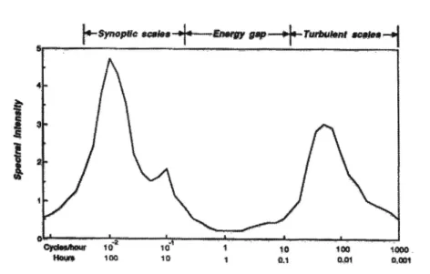
(1957) showing the relative contributions to horizontal wind speed variations (“spectral intensity”) from synoptic and turbulent scales of motion. . . . 27 1.3 Photograph of wake clouds generated by the Horns Rev wind

farm. (Christian Steiness, 2008, Vattenfall) . . . . 27 1.4 The effect of turbulence intensity on the reduction in wind speed

(% deficit) behind a given wind turbine at a certain wind speed as a function of the wind turbine rotor diameter, D (source: adapted from the figure 2 of Elliott (1991)). . . . 28 2.1 Sea (ocean) surface drag coefficients at 10 m as a function of

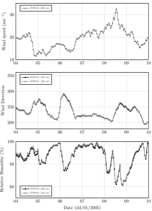
the 10 m neutral wind speed as reported by Merzi and Graf (1988), Janssen (1997) and Dobson et al. (1994). Also included is Charnock’s parametrization, eq. (2.12) for α = 0.018. . . . . . 41 2.2 Wind speeds at 80 m (top), wind direction at 90 m and 33 m

(middle) and relative humidities at 90 and 33 m (bottom) as recored at FINO1 during January 4–10, 2005. . . . 44 2.3 Friction velocities (top) and vertical standard deviations (middle)

at 80 and 40 m, and Obukhov lengths as estimated from the 40 m sonic (bottom) as recorded at FINO1 during January, 4–10. . 45 2.4 Top: Friction velocities (left) and drag coefficients (right) as a

function of wind speed using u

estimated from the 40 m sonic during January 4–10, 2005. Bottom: Measurements of drag coef- ficients (left) and friction velocities (right) as reported by Dobson et al. (1994). The solid line is Charnock’s law for α = 0.018 and the dashed line is a regression in u

= f (U

) space based on the FINO1 measurements (i.e., top left). . . . 46 2.5 Average wind profiles during the 5th (top) and 7th (bottom)

of January 2005 compared with equivalent neutral wind profiles assuming β = 5 (left) and β = 10 (right) in eq. (2.39). . . . 47 2.6 Wind speeds at 80 m (top), wind direction at 90 m (middle) and

relative humidities at 90 and 33 m (bottom) at FINO1 during February, 20–28, 2005. . . . 49

15

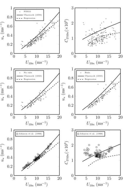
2.8 Average wind speed profiles during the 23rd (left) and 25th (right) of February 2005 compared with equivalent neutral wind profiles (solid black curve) and the unstable profiles from Monin-Obukhov similarity theory based on the 40 m sonic and cup anemometers. 51 2.9 Top: Friction velocities (left) and drag coefficients (right) as a

function of wind speed as measured at FINO1 between February 20-28, 2005. Middle: Measurements during this same period with no rain detected at the 20 m measurement (left) and with rain de- tected at the 20 m measurement (right). Bottom: For comparison are measurements of u

and C

as a function of wind speed in the Baltic as reported by Johnson et al. (1998). The solid line is Charnock’s law for α = 0.018, the dashed is a regression for a

= (0.042, −0.01) using all measurements. . . . 52 2.10 Roughness Reynolds number (top) and C

(bottom) as a func-

tion of wind speed during Janaury 2005 (left) and February 2005 (right). The two solid lines (top) are for Re

= 300 and 3. The solid line (bottom) is Charnock’s parametrization for α = 0.018.

The dashed curves are eq. (2.36) for a

= (0.057, −0.26) (left) and (0.042, −0.01) (right). The dotted line is eq. (2.40) after Amorocho and Devries (1980). . . . . 53 2.11 Wind speeds at 80 m (top), wind direction at 90 m (middle)

and relative humidity at 90 and 33 m (bottom) at FINO1 during November, 9–15 2005. . . . 55 2.12 Friction velocities (top) and vertical velocity standard deviations

(middle) at 80 and 40 m and Obukhov lengths from the 40 m sonic (bottom). . . . 56 2.13 Friction velocities (left) and drag coefficients (right) as a function

of wind speed as measured at FINO1 between November 9–15, 2005 (top) and measurements reported by Anderson (1993) (bot- tom). The solid line is Charnock’s law for α = 0.018. The dashed curve is the linear regressions in u

= f (U

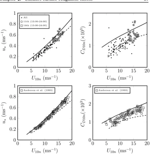
) space for measure- ments in the top left figure. . . . 57 2.14 Average wind speed profiles during the 11th (13:00 – 24:00) (left)

and 14th (13:00 – 24:00) (right) of November 2005 compared with equivalent neutral wind profiles (solid black curve) and the stable (left, β = 10) and unstable (right) profiles from Monin-Obukhov similarity theory based on the 40 m sonic and cup anemometers. 58 2.15 The drag coefficient as a function of the 10 m wind speed accord-

ing to Charnock (1955)’s parametrization for α = 0.018 (solid line). The squares with error bars are the estimates of Powell et al. (2003) using radiosonde profiles in tropical cyclones. Gray dots are direct aircraft measurements reported by French et al.

(2007). The curves corresponding with the January, February and

November, 2005 measurements defined according to eq. (2.36) for

the linear regression constants specified in the text. . . . 59

3.1 Illustration of Toba’s

law showing the measurements at FINO1 during January 4–10, 2005 and February 20–28, 2005 and the line defined by eq. (3.7) for B = 0.06. . . . 65 3.2 Left: The figure 9.19 from Munson et al. (2002) with some as-

pects removed showing the relationship between the drag coef- ficient and aspect ratio for an ellipse of length ` and height D.

Right: The relationship between the offshore drag coefficient de- rived from eq. (3.16) (gray dashed line), a constant drag coeffi- cient assuming C

= 0.03 (dashed black line) and a correlation equation between these two (solid black line). . . . 67 3.3 Eq. (3.22) on logarithmic axes for various exponents n (adapted

from the figure 1 of Churchill and Usagi (1972)). . . . 68 3.4 A working plot for correlation based using eqs. (3.22) and (3.23)

(adapted from the figure 2 of Churchill and Usagi (1972)). . . . . 68 3.5 Y versus Z (left hand side) and

versus

(right hand side)

as calculated at FINO1 for the periods during January (top), February (middle) and November (bottom) 2005 as calculated for various n (1, 2, 3, 4 and ∞) based on eqs. (3.22) and (3.23).

Here, Y =

1/2 D10n

Hs λp

and Z =

λp

. . . . 71 3.6 Drag coefficients as a function of one-tenth aspect ratios dur-

ing January and February 2005. The solid black, dashed gray and dashed gray lines are the correlation equation, eq. (3.27) the wave steepness asymptote (3.16) and the constant drag coeffi- cient asymptote (3.19). The top figure shows bin averages and the bottom figure shows one hour means. . . . . 72 3.7 January 2005 (top), February 2005 (middle) and November 2005

(bottom): Drag coefficients as measured from the FINO1 tower compared with C

inferred from buoy measurements accord- ing to the correlation eq. (3.27) (top), the asymptotic relations, eq. (3.28) and (3.29) (middle), and the correlation equation again (bottom). . . . 74 3.8 Top: Phase diagram of C

against

s

from January 4–5th, 2005. A period within this period is indicated by black bullets for the 4th (14:00) to the 5th (5:00) illustrating the scaling with eq. (3.16) during this time. Bottom: Wind (33 m) and wave di- rections during the same period, also showing the black bullets corresponding with those in the phase diagram. . . . 75 3.9 Y versus Z (left hand plots) and

versus

(right hand plots)

for n = 1, 2, 3 and 4 according to eqs. (3.22) and (3.23) where Y = C

/

p

and Z = 0.03/

p

. Top: Measurements reported by Janssen (1997) in the North Sea and SCOPE measurements exposed to the open Pacific Ocean. Middle: Measurements re- ported by Dobson et al. (1994) in the North Atlantic. Bottom:

Measurements reported by Merzi and Graf (1988) and Johnson

et al. (1998) over Lake Geneva and in the Baltic Sea, respectively. 76

surements, plotted as a function of one-tenth of the aspect ratio,

λ_p

10Hs

. Also included are functions corresponding to eq. (3.8) for C

= 0.03 (gray dashed line), eq. (3.16) (black dashed line) and eq. (3.27) (solid black line) which is an interpolating function between the two asymptotes. Bottom: Same as the top figure but focused on the low aspect ratio region and the scale of both axes are linear. . . . 77 3.11 Top: Estimates of C

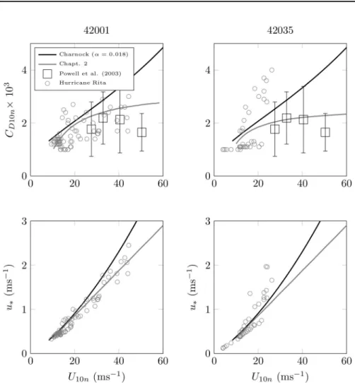
as a function of wind speed calculated

using eq. (3.27) using measurements from buoys located in the Mexican gulf (stations 42001 (left) and 42035 (right)). For com- parison are the estimates in tropical cyclones from Powell et al.

(2003), Charnock’s parametrization for α = 0.018 and eq. (3.30) for (a

= (0.057, −0.26) (January, 2005 at FINO1). Bottom:

The corresponding plots of friction velocities as a function of wind speed. Buoys 42001 and 42035 correspond with the periods 21–24 September and 23–25 September 2005, respectively. . . . 79 4.1 The figures 1a and 1b from Garratt (1987) showing the growth

of an internal boundary layer as warm continental air flows over a cold sea (a) and the corresponding vertical profiles of potential temperature over land (θ

) and over sea (θ

) (b). . . . 84 4.2 Adapted from the figure 2 from Brooks and Rogers (2000) show-

ing wind speed and virtual potential temperature profiles recorded by aircraft at two different locations over the Persian Gulf during the passage of a stable internal boundary layer. . . . 86 4.3 The 151 x 151 (10 km resolution) domain centered on FINO1. . . 87 4.4 DWD surface pressure map (as archived by Wetter3.de) on in-

dicative of the period 04/05/06 - 11/05/06 (here 07/05/06 6 UTC) showing a high over Scandinavia and low just east of Ire- land (left). The estimated geostrophic wind at FINO1 for the entire period (right). . . . 89 4.5 Wind speed according to the 80 m cup anemometer compared

with the 80 m wind speed according to the WRF model (top).

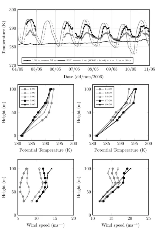
Wind direction at 90 and 33 m as measured by wind vanes at FINO1 (middle). Relative humidity as measured at 90, 50 and 33 m by hygrometers at FINO1 (bottom). . . . 91 4.6 Time series of temperature at 100 m, 33 m and the sea surface

(SST) at FINO1 in comparison with the modelled 2 m temper- ature over land directly east of FINO1 (top). The dashed line shows the modelled temperature shifted three hours forward. Po- tential temperature (middle) and wind speed profiles (bottom) during the 4th as shown every second hour (UTC). . . . 92 4.7 Heat fluxes (top), turbulence intensities (middle) (eq. (4.19)) and

local friction velocities (bottom) (eq. (4.17)) at 80, 60 and 40 m

at FINO1. . . . 97

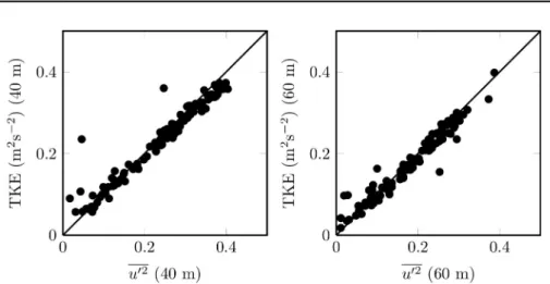
4.8 Comparison between the TKE and streamwise variances as mea- sured at 40 (left) and 60 m (right) during the period May 4-11, 2006. . . . 98 4.9 TKE

at FINO1 assuming TKE ≈ u

and u

from u

interpo-

lated to the surface using eq. (4.21) The scaling is compared with that performed by Caughey et al. (1979) (it is their solid curve from their figure 5 (top left)). . . 100 4.10 Scaled TKE during the 10th from 6:00 – 20:00 similar to that

performed in Fig. 4.9, but concentrating on the 40 m measure- ment (top left). Also shown that are the times 12:00 and 18:00 indicating the departure from outer scaling. TKE

as a func- tion of the local Monin-Obukhov stability parameter indicating illustrating instability between 12:00 and 18:00 (top right). Wind speed profiles from 8:00 – 13:00 (bottom left) and from 14:00 – 19:00 (bottom right). . . 101 4.11 Drag coefficients as estimated from buoy measurements using eq.

(4.26) compared with the MYJ model (top). Local friction veloc- ities at 40 m (middle). Wind (33 m) and wave directions (bottom).102 4.12 Time series of the difference between the rate of change of wind

and wave direction (5 hour moving average) compared with 50 times the rate of change of the drag coefficient estimated from buoy measurements plus 9 hours in time (also a 5 hour moving average). . . 103 4.13 Scaled TKE (TKE

) as calculated by the MYJ model assuming

TKE ≈ u

. The periods here correspond with those in Fig. 4.9 above. . . 104 4.14 Absolute TKE and turbulence intensity as measured at FINO1

and calculated by the MYJ model. . . 105 4.15 Velocity profiles at FINO1 during the 4th (top), 6th (middle)

and 8th (bottom) at various times in comparison with the MYJ model and when using an extra 6 levels less than 100 m. . . 106 5.1 Left: Adapted from the figure 1 of Mellor and Yamada (1982)

interpreting the measurements of scaled horizontal velocity fluc- tuations as reported by Perry and Abell (1975) (their figure 7) for different Reynolds numbers. The horizontal line corresponds with u

= 4.49. Right: Adapted from the figure 7 (top) of DeGraaff and Eaton (2000) showing measurements for a range of Reynolds numbers and a lack of an obvious choice for u

. . . 115 5.2 The figure 5 of Grant (1986) showing aircraft measurements of

horizontal (a), lateral (b) and vertical (c) variances (σ

) nor- malised by the friction velocity and plotted against the height, z which itself has been normalised by the boundary layer height, z

. The “P” and “S” along the horizontal axis refer to the measure- ments of Panofsky et al. (1977) and Smith (1980), respectively.

The solid lines are based on the aircraft measurements of Nicholls and Readings (1979). . . 115 5.3 Calculation of Φ

and Φ

in stable stratification according to

eqs. (5.31) and (5.32) for various γ

and surface length scale, `

as defined in the text. . . 119

q

for the year 2005 at FINO1 as a function of stability. The error bars are two standard deviation width. Comparison the LES results of Nakanishi (2001) are also included. . . . 121 5.6 The relationship between Ri

and B

as calculated from eq. (5.46)

for a range of γ

. . . 123 5.7 Left column: Time series of 10 and 50 m wind speeds and TKE

from single column model simulations using the current MYJ model, that defined in Mellor and Yamada (1982) (MY82), an example of physical unrealistic simulation where γ

= 0.2 and B

= 26 (MYJg1) and an alternative MYJ versions using γ

= 0.27 and B

= 26 (MYJv2). Right column: The same cases as the left column showing profiles of wind speed, TKE and K

at 3:00 local time. The observations are those taken from the main tower during the CASES-99 experiment. . . 125 5.8 Left column: Time series of 10 and 50 m wind speeds and TKE

from single column model simulations using γ

= 0.27. Right column: The same cases as the left column showing profiles of wind speed, TKE and K

at 3:00 local time. The observations are those taken from the main tower during the CASES-99 experiment.126 5.9 Left: The dependence of the maximum K

throughout the bound-

ary layer at 3:00 local time on Ri

for MYJ, MY82 and MYJ (with γ

= 0.27, B

= 26 and c = 2.7). Right: The dependence on this same K

on γ

and c at constant Ri

. . . 127 6.1 Vertical profiles of turbulent kinetic energy normalised by the

friction velocity as calculated by MYJ and MY82 and compared with the curve of Caughey et al. (1979) as presented in their figure 5 (top left). The height, z has been normalised by the estimated internal boundary layer height (see Chapter 4). . . 135 6.2 Vertical profiles of turbulent kinetic energy normalised by the

friction velocity as calculated by MYJ and g127b128 and com- pared with the curve of Caughey et al. (1979) as presented in their figure 5 (top left). The height, z has been normalised by the estimated internal boundary layer height (see Chapter 4). . . 136 6.3 Wind speed at 80 m as calculated by MYJ (top), MY82 (mid-

dle) and g127b128 (bottom) in comparison with both MYJ and FINO1 measurements. . . 137 6.4 Turbulence intensity as calculated by MYJ (top), MY82 (mid-

dle) and g127b128 (bottom) in comparison with both MYJ and FINO1 measurements. . . 138 6.5 Wind speed (left) and TKE (right) profiles on May 4th at 22:00

for different critical Richardson numbers, Ri

. . . 140 6.6 Wind speed and TKE (absolute) profiles on May 4th at 12:00

(left) and 22:00 (right) as calculated by MYJ, MY82 and g128b128

compared with FINO1 measurements. . . 142

6.7 Wind speed and TKE (absolute) profiles on May 6th at 15:00 (left) and 22:00 (right) as calculated by MYJ, MY82 and g128b128 compared with FINO1 measurements. . . 143 6.8 Wind speed and TKE (absolute) profiles on May 8th at 15:00

(left) and 22:00 (right) as calculated by MYJ, MY82 and g128b128 compared with FINO1 measurements. . . 144 6.9 Profiles of WRF calculated TKE

according to MYJ (left) and

g127b128 (right) as a function of the height normalised by the boundary layer height,

i

in comparison with the results of Caughey et al. (1979) and the FINO1 measured TKE

at 40, 60 and 80 m during January 4–10, 2005. . . 145 6.10 Hub height (80 m) wind speeds (left column) and turbulence

intensity (right column) as measured by FINO1 in comparison with MYJ (top), MY82 (middle) and g127b128 (bottom). . . 146 6.11 Average profiles at FINO1 during January 5th (top left) and

7th (top right) compared with MYJ and g127b128. The drag coefficient as a function of the aspect ratio (bottom left) and wind speed (bottom right) at FINO1. Highlighted in these fig- ures are the points corresponding with the 5th (circles) and the 7th (squares). Bottom left: Solid black line is eq. (6.6); dashed black line is eq. (6.7); dashed gray line is eq. (6.8). Bottom right:

The solid black line is Charnock’s parametrization and the solid gray line is eq. (6.10) for a

= (0.058, -0.28). . . 147 6.12 Wind speeds at 80 m (top), Wind (33 m) and wave directions

(middle) and Turbulence intensity (bottom) during February 20–

28, 2005. . . 149 6.13 Top: Average wind speed profiles during the 22nd (left) and 23rd

(right) as calculated by the standard MYJ model and compared with a modified roughness length (MYJzo) defined according to eq. (6.10), compared with average wind speed profiles at FINO1.

Bottom left: Drag coefficients as a function of the aspect ratio.

The solid black line is eq. (6.6); dashed black line is eq. (6.7);

dashed gray line is eq. (6.8). Highlighted by circles and squares are points during the 22nd and 23rd, respectively. Bottom right:

Drag coefficients as a function of wind speed. The solid black lines correspond with MYJ while the solid gray lines MYJzo. . . 150 6.14 A direct comparison between the 80 m Ti as calculated by MYJ

(left) and g127b128 (right) during February 20-28, 2005. . . 151 6.15 November 9-16, 2005: Wind speeds at 80 m (top), wind (33 m)

and wave directions (middle) and turbulence intesity (bottom). . 152 6.16 Top: Wind speed profiles for two 12 hour periods on the 11th (left)

and 14th (right) November 2005 comparing profiles at FINO1 with the standard MYJ model and with a modified roughness (MYJzo) using eq. (6.10). Bottom: Drag coefficients for the en- tire 9-16 November period where the two 12 hour periods are highlighted as circles (11th) and squares (14th) as a function of one-tenth the aspect ratio (left) and the 10 m wind speed (right).

Bottom left: The dashed and solid curves are defined in the text.

Bottom right: The black and light gray curves correspond with

MYJ and MYJzo, respectively. . . 153

4.1 Calculation of the internal boundary layer height, h between 11:00 and 23:00 for the 4th, 6th, 7th and 8th according to eq.

(4.6) using estimated geostrophic wind speeds shown in Fig. 4.4 and x = 150 km. Here, δ corresponds with the height of the low level jet (LLJ). . . . 94 5.1 Turbulence statistics from some recent laboratory boundary layer

experiments by ¨ Osterlund (1999) and Carlier and Stanislas (2005) and a years worth of measurements at FINO1. The magnitude of γ

is based on either eq. (5.15), (5.16) or (5.17) for u

, v

and w

, respectively. . . 118 5.2 Summary of different cases tested in the single column model

below. The constants are defined in the text. Ri

is the critical Richardson number as determined from the constants. . . 124

23

Introduction

1.1 Introduction

Wind energy is proposed to partly replace finite fossil fuel resources whose con- sumption results in the emission of annually increasing amounts of greenhouse gases, depending on the level of economic activity (Friedlingstein et al., 2010).

One estimate has worldwide coal production peaking in 2030 (Mohr and Evans, 2009), which if true, gives net energy importing regions such as the entire Euro- pean Union apart from Denmark

approximately 20 years to find a replacement for this energy shortfall.

Wind energy is a renewable energy resource and thus it is proposed that off- shore wind energy can provide at least one non-traditional, industrial scale en- ergy source to meet future conventional energy production shortcomings where 150 GW of offshore wind energy is targeted by 2030 in Europe (EWEA, 2011).

While wind energy itself does rely on fossil fuels at least during the construc- tion phase, the use of other non-traditional fossil fuel emitting energy sources are also proposed as large scale energy shortfall replacements (e.g. tar/oil sands, S¨ oderbergh et al., 2007). However, these come with the further disadvantages of an increase in greenhouse gas emissions again (e.g. Brandt and Farrell, 2007), and their own current technical problems and future production shortcomings (Mohr and Evans, 2010).

While wind speeds are generally higher and steadier offshore compared with that over land, there are additional technical and financial challenges associ- ated with offshore wind energy compared with that onshore (Breton and Moe, 2009). One particular problem related to this work is the state of the sea in that particular wave and weather conditions offshore limits the times to which offshore sites can be accessed. For example, access via the sea to the FINO1 research platform (FINO: “Forschungsplattformen in der Nord- und Ostsee”) located roughly 45 km of Borkum Island in the German Bight is limited when significant wave heights are greater than 1.5 m (K¨ uhnel and Neumann, 2010).

Work presented in this thesis will be centered on measurements recorded at the FINO1 platform, which is also located near the “alpha ventus” wind farm consisting of twelve 5 MW wind turbines. The site is unique in that it is lo- cated further out to sea than wind farms in other areas in order to protect the

1http://epp.eurostat.ec.europa.eu/statistics explained/index.php/Main Page

25

Figure 1.1: Photograph of the FINO1 platform (source: bundesregierung.de).

sensitive coastal ecology in this area (www.alpha-ventus.de). This represents an opportunity to investigate offshore meteorological conditions not regularly in- vestigated in the past and that are further relevant for wind energy applications.

While the wind turbines have only been in place at alpha ventus since 2009, the FINO1 platform itself has been monitoring conditions since 2003 (Neumann et al., 2010), where some measurement periods during 2005 and 2006 will be considered in this work.

The FINO1 tower extends 100 m above the sea surface and sits on a platform, itself located about 20 m above the surface as illustrated in Fig. 1.1. While the conditions displayed in Fig. 1.1 appear calm, to illustrate the harsh conditions that can be encountered at this site, the structure just below the platform has in the past been damaged as a result of wave action during high wind events (Outzen et al., 2008). FINO1 is equipped with a broad range of meteorological and oceanography instruments, where the measurements used in this thesis have come out of the work of T¨ urk (2008).

Equipment of particular relevance here are the wind speed measurements at 10 m vertical intervals between 30 and 100 m and turbulence measurements at 40, 60 and 80 m, while wave field information has been provided separately by the German maritime and hydrographic agency (BSH). A number of par- ticularly high wind speed periods at FINO1 will be investigated in this thesis and compared with results reported in the literature and numerical simulations.

The broader aim here is a deeper understanding of the behaviour of offshore

meteorological parameters encountered at a site such as FINO1 relevant for

wind energy purposes. It is intended that the work presented here will not just

be useful towards further understanding the meteorological conditions at other

offshore wind energy sites currently being developed in the North Sea even fur-

ther from the coast than alpha ventus (www.offshore-wind.de), but also at other

offshore sites around the world.

Figure 1.2: The figure 2.2 from Stull (1988) as adapted from Van der Hoven (1957) showing the relative contributions to horizontal wind speed variations (“spectral intensity”) from synoptic and turbulent scales of motion.

Figure 1.3: Photograph of wake clouds generated by the Horns Rev wind farm.

(Christian Steiness, 2008, Vattenfall)

1.2 Problem Definition

While from fundamental analysis it can be found that the available wind power, P

for a single wind turbine will be proportional to the third power of the wind speed, u by

P

= 1

2 ρAu

, (1.1)

this relationship will be complicated from a meteorological perspective by the

effects of turbulence. Here, ρ is the air density and A is the turbine rotor cross-

sectional area. Fig. 1.2, which is the figure 2.2 from Stull (1988) as adapted from

Van der Hoven (1957), illustrates the time scales one can expect will influence

Figure 1.4: The effect of turbulence intensity on the reduction in wind speed (%

deficit) behind a given wind turbine at a certain wind speed as a function of the wind turbine rotor diameter, D (source: adapted from the figure 2 of Elliott (1991)).

variation of the wind speed. It can be seen that the wind speed will vary mostly over scales of days (O(100) hours) and minutes, attributable to synoptic scale events and to turbulence, respectively. From a wind energy perspective, the amount of turbulence is quantified via the turbulence intensity. For example, one can define a wind speed fluctuation, u

that deviates from the wind speed averaged over time T ,

U = 1 T

Z

udt, (1.2)

by

u = U + u

(1.3)

such that the average of all fluctuations during this period 1

T Z

0

u

dt = 0. (1.4)

From Fig. 1.2, the averaging time T is chosen to be approximately 10 minutes to capture the turbulent scales of motion while avoiding synoptic scales via the “energy gap” which is O(1) hour. The mean wind speed U will then vary depending on the synoptic scale motion on time scales greater than 1 hour.

The turbulence intensity then first enters directly into the problem by taking the average of the wind speed raised to the third power to give (Devries, 1979)

u

= 1 T

Z

(U + u

)

= U

+ 3U

u

+ 3U u

+ u

, (1.5) where the second term on the right hand side is neglected, i.e.

u

= U

1 + 3 u

U

+ u

U

!

, (1.6)

because of eq. (1.4). Assuming that the velocity probability distribution is sym- metric, then

u

= U

1 + 3Ti

, (1.7)

where the turbulence intensity is defined as Ti =

p u

U . (1.8)

Hence, given a Ti of about 20%, then u

can differ from U

by about 10%.

On the one hand, offshore turbulence intensities will often be much lower than 20% even in high wind speeds as will be shown in this thesis. On the other hand, offshore wind turbines will be located within a wind farm so that the actual Ti as seen by a turbine within a farm will likely be enhanced over the free stream Ti given by eq. (1.8) due to the wakes produced by other wind turbines. Wind turbine wakes are readily seen in the famous photograph taken by Christian Steiness of the Horns Rev wind farm in the Danish sector of the North Sea reproduced here in Fig. 1.3. The wakes are able to be seen here due to the advection of cold air over warm water, which due to the particular air-sea temperature difference, resulted in saturated air behind the turbines on account of the enhanced turbulent mixing (Emeis, 2010a). An example of the measured wind speed reduction within turbine wakes can be illustrated in Fig.

1.4 as reported by Elliott (1991) for an onshore wind farm. Fig. 1.4 shows the velocity deficit, that is the percentage difference in wind speed behind a wind turbine compared with the free stream wind speed, as a function of the distance behind the wind turbine rotor in the scale of the rotor diameter, D. It can be seen that the difference between the free stream and wake wind speeds decreases with increasing distance and with increasing turbulence intensity. The higher turbulence intensity will imply an enhanced mixing between the free and wake streams, and a quicker wind speed recovery behind the turbine.

While Fig. 1.4 shows measurements recorded onshore, the problem consid- ered in this thesis concerns the calculation of the meteorological parameters, U and Ti for conditions offshore. For example, due to the high capital costs, offshore turbines will most likely be located within wind farms and will possibly be relatively closely spaced so that an accurate calculation of both U and Ti is necessary for wind power assessment. One example are the turbines within the Nysted offshore wind farm south of Lolland Island, Denmark where turbines are spaced within 10 rotor diameters of each other (Barthelmie et al., 2007). From a meteorological perspective, the offshore environment at FINO1 is complicated by the interaction with the coast (despite FINO1 being 60 km from the main- land), the generally lower surface roughness encountered offshore (although this is non-linearly dependent on the wind speed) and the lower turbulence intensi- ties over water compared with over land (Lange, 2007).

The aim of the work to be presented here is to achieve a better calculation of

the offshore parameters, U and Ti in hope that this will help forecasters better

anticipate the expected wind energy power output from offshore wind farms. For

example, the exact dependence of offshore surface roughness on atmospheric and

sea parameters is a well known (Jones and Toba, 2001) and ongoing problem

(Sullivan and McWilliams, 2010) which will be shown in this work to have

consequences for the precise calculation of the offshore wind speed.

partial differentials. To solve these equations, a numerical model is generally employed, but given the finite nature of computing resources, all scales of motion (at least from the perspective of wind energy) can still not possibly be resolved.

Some of the relevant processes, especially turbulence, occur towards the earth’s surface where the scales of motion take place within the finite bounds of the numerical differencing grid, but nonetheless influence the large scale solution so that neglecting their influence is not possible. In these situations one must retreat to statistics in conjunction with similarity solutions to describe these processes.

The effect of turbulence on the large scale solution for the wind speed can be seen via the conservation of momentum equation using index notation, which after a Reynolds decomposition (Stull, 1988) gives

∂U

∂t + U

∂U

∂x

= −δ

g + f

U

− 1 ρ

∂P

∂x

+ ν ∂

U

∂x

− ∂u

u

∂x

. (1.9)

Here, P is the average atmospheric pressure, g is gravity, f

is the Coriolis parameter, ν is the kinematic viscosity, δ

is the Kronecker delta, is the alternating unit tensor.

Vastly simplifying eq. (1.9) is possible by assuming a steady, horizontally homogeneous flow parallel with the x

direction in the absence of a pressure gradient (Lumley and Panofsky, 1964). Assume then that we are sufficiently close to the surface such that Coriolis effects are small, but not too close so that viscosity begins to be influential so that eq. (1.9) reduces to

− ∂u

w

∂z = 0. (1.10)

After integrating eq. (1.10) and then multiplying by the air density, one obtains the surface stress

τ = −ρu

w

, (1.11)

from which results the most common boundary layer, turbulent velocity scale, the “friction velocity”

u

= r τ

ρ . (1.12)

In practice, the average wind speed and surface stress are often not perfectly aligned so that the friction velocity is estimated by

u

=

u

w

+ v

w

. (1.13)

While eq. (1.9) did not yield any explicit solution, it did give us a scaling

velocity, u

which as we will see in the following chapters, exerts its influence

on processes throughout. With the known scaling parameters, then similarity

solutions can be found which with the help of measurements, results in explicit

solutions that can consequently be used in parametrizations in more complex ap-

plications, e.g. numerical weather prediction. Perhaps the most famous of these

is the logarithmic velocity profile which describes the lowest level in numerical models and often the flow up to the hub height of wind turbines. In arriving at eq. (1.10), we assumed that the relevant length scale of interest is the height above the surface, z (in fact it explicitly appears in eq. (1.10)). Depending at what height we want to focus on above the surface, there are at least a couple of other possible length scales: as z → 0, there is a “dissipative” length scale,

ν

u∗

and as u

w

→ 0, we define an “outer” length scale, δ.

If in practice we assume after Barenblatt (1993) that the velocity gradient can possibly depend on all these length scales then

∂U

∂z = f (u

, z, ν, δ) , (1.14) where f is here and throughout, an arbitrary function. Here we have 5 vari- ables in 2 dimensions (length, time) and hence by Buckingham’s Π theorem, 3 dimensionless groups result:

Φ

= f (z

, Re

) , (1.15)

where Φ

=

∗

∂U

∂z

is the dimensionless wind shear, z

=

is the “wall coordinate” and Re

is the Reynolds number based on the outer length scale.

In atmospheric flows, both Re

and z

are necessarily very large so that we can make the assumption that (Barenblatt, 1993) f → κ

as Re

→ ∞ and z

→ ∞, where κ is von Karman’s constant.

Integrating eq. (1.15) then gives us the logarithmic velocity profile U

u

= 1

κ ln zu

ν

+ C, (1.16)

where von Karman’s constant and the constant C are then apparently universal, and thus a similarity solution has been found for all flows abiding by the as- sumptions made above. Eq. (1.16) can be further modified in atmospheric flows to account for a surface roughness much larger than the dissipative length scale.

A roughness length scale, z

is then used which also accounts for the decreasing C as the roughness increases:

U u

= 1

κ ln z

z

. (1.17)

Eq. (1.17) is the foundation on which the theory of boundary layer turbulence is built and how it is represented in numerical models. It can be seen that similarity concepts are especially valuable in this field and will be used throughout this work beginning with treatment of the roughness length scale z

in Chapter 2.

1.4 Scope

The following thesis is aimed at investigating to what effect the nature of offshore

meteorology will affect the calculation of offshore meteorological parameters

relevant for wind energy. The nature of the sea surface itself via its characteristic

roughness length, z

as defined through the logarithmic velocity profile will play

a major role and this will be considered initially in Chapter 2 (Offshore surface

roughness effects during high wind speeds at FINO1). There, the roughness

offshore drag coefficients) where a first-order scaling of roughness effects based on the measured wave field at a buoy near FINO1 will be presented. While the scaling is able to successfully describe both measurements at FINO1 and those reported previously in the literature, departures from the expected scaling behaviour will lead to further investigations in Chapter 4.

The work in Chapter 4 (Air-Sea and land interaction effects at FINO1) presents an analysis of a particular flow during the spring of 2006 which re- sulted in a diurnal cycle in detected meteorological parameters by FINO1. Di- urnal cycles are not as commonly detected offshore compared with onshore due to the resistance of the water surface to solar heating, but certain flow situations leading to interactions with the coast are to be expected at FINO1 as will be demonstrated here. With the nature of this flow, the interaction between the air and the sea can be uniquely investigated. For example, the scaling results of Chapter 3 can be used to investigate the roughness lengths during this period, where the wave field properties are also found to experience a periodic be- haviour. This flow also allows investigation of the vertical structure of offshore turbulence over a good portion of the boundary layer, since the outer length scale, δ is found to be not much higher than the tower during most of this pe- riod. A comparison with numerical simulations shows clear differences between the turbulence anticipated by the model and FINO1 measurements, which re- sults in underpredicted modelled wind speeds and leads to an investigation of the model in Chapter 5.

Chapter 5 (Mellor-Yamada-Janji´ c model modifications in WRF) investigates more closely one particular boundary layer parametrization scheme (the Mellor- Yamada-Janji´ c (MYJ) model) in the Weather Research and Forecasting (WRF) model. It will be shown that the misrepresentation of turbulence detected at FINO1 by this model as shown in Chapter 4 is a consequence of both theo- retical (similarity theory) and practical limitations. With regards to practical limitations, an alternative way of specifying the model closure assumptions is proposed and demonstrated to give realistic results in the single column model within the WRF model. Tests in three-dimensional simulations are left to Chap- ter 6.

Chapter 6 (Applications for wind energy: Accounting for offshore rough- ness and turbulence intensity) will then bring the work initiated in Chapter 2 together to show potential benefits in the calculation of wind speed and tur- bulence intensity based on the preceding 4 chapters. However, it will be shown that there is still work to be done if an optimal anticipation of offshore wind power is to be attained. This is done by revisiting the high wind speed periods considered in Chapters 2 to 4, including the spring 2006 period. In all these periods an improved calculation of turbulence is demonstrated using changes to the MYJ model proposed in Chapter 5. Wind speeds also show some im- provement, but there is clear room for further improvement where the exact reason for this will be identified. It will be demonstrated that wind speeds can also be improved with a precise consideration for the offshore surface roughness.

This will however require a higher order analysis than that performed here in

order for further progress in this area to be made. However, it is believed that

this thesis has laid out a pathway for further improvement in the calculation of

offshore meteorological parameters from a wind energy perspective, as will be

concluded in Chapter 7 (Conclusions).

Offshore surface roughness effects during high wind speeds at FINO1

2.1 Introduction

This work will begin by analysing the nature of the surface roughness encoun- tered offshore, which as one could imagine is appreciably different from that experienced over land. The surface roughness evolves with the speed of the air flow above and is usually parametrized using some variant of the classic Charnock (1955) parametrization to be defined below. Given the difficulties with modelling surface features over land surfaces (Raupach et al., 1991), it is believed that “over oceans, the drag laws are a bit easier to parameterize...”

(Stull, 1988). However, there are also difficulties over water at, for example, very high wind speeds as experienced in tropical cyclones where a contradiction with Charnock’s parametrization is believed to exist (Powell et al., 2003). At very low wind speeds, the water surface can be much smoother than that over land which means the parametrization must be further adapted for such situations.

From the perspective of numerical weather prediction models, the impor- tance of an accurate parametrization for wind energy purposes is crucial since the nature of the roughness determines the lower boundary of the theoretical logarithmic velocity profile. On a global scale, since the majority of the world’s surface is water, accurate offshore roughness parametrizations extend to other applications in meteorology and climatology.

The Charnock (1955) parametrization will be the starting point in this chap- ter for analysing the surface roughness at FINO1. Three relatively high wind speed periods which took place at FINO1 during 2005 will then initiate the investigation of the surface roughness at FINO1. The results of that study will then be compared with some results reported previously in the literature. From this analysis, an alternative drag law will be suggested which further explains the anticipated offshore surface roughness in tropical cyclone wind speeds better than Charnock (1955). These results will then lead to a more detailed treatment in the next chapter.

35

everyday language, “roughness” is possibly something one more associates with solid surfaces, but it has meaning over water in the sense of a logarithmic velocity profile. In that sense it is often called “aerodynamic roughness” to distinguish it from actual roughness. Since the roughness of the water surface evolves with the state of the atmosphere above, the challenge over water surfaces is then to parametrize the aerodynamic roughness based on bulk air side properties.

The most successful parametrization at this so far is due to Charnock (1955) whose work is widely used in numerical models. However, the Charnock (1955) parametrization does encounter difficulties at low wind speeds when the surface roughness is small (Smith, 1988), at very high wind speeds in tropical cyclones (Powell et al., 2003) and at intermediate wind speeds where there is uncertainty in the empirical constant (Fairall et al., 2003).

In the following section, offshore roughness will be introduced via classi- cal concepts developed with respect to laboratory flows. This will lead to an introduction of the drag coefficient as used for offshore flows. The effects of stratification on the drag coefficient will then be considered. Out of these con- cepts will come Froude number scaling with which the marine drag coefficient is usually scaled. It will then be shown that Froude number scaling fails to collapse measurements from a number of different sources.

2.2.1 Offshore roughness

The starting point for analysis here is the logarithmic velocity profile introduced in the previous chapter

U u

= 1

κ ln zu

ν

+ C, (2.1)

valid in the absence of any appreciable surface roughness, where von Karman’s constant, κ and the integration constant, C are in theory universal. As the surface becomes rougher relative to the height of the inner length scale,

there is a greater sink of momentum at the surface and the constant C in eq.

(2.1) becomes a decreasing function of the size and spacing of the roughness elements. In this case, the logarithmic velocity profile is given by

U u

= 1

κ ln z

k

+ 8.5, (2.2)

where k

is the height of the roughness elements used in laboratory experiments performed by Nikuradse (1933), where pipes were artificially roughened with sand. Eq. (2.2) is valid for a so-called completely rough surface which is based on a roughness Reynolds number,

Re

= u

k

ν , (2.3)

and is said to occur for Re

& 70, while a smooth regime where eq. (2.1) is

valid is entered for Re

. 5. A transitional roughness regime occurs between

these two extremes, where the behaviour of the surface roughness is much more

ambiguous (Bradshaw, 2000).

Rewriting eq. (2.1) as a roughness length scale, z

, i.e. the “aerodynamic roughness” gives

U u

= 1

κ ln z

z

, (2.4)

which equating with eq. (2.2) gives a relationship between the equivalent sand grain roughness and z

as

k

≈ 30z

. (2.5)

From eq. (2.3), the fully rough regime is said to occur (Lange et al., 2004) for an aerodynamic roughness Reynolds number

Re

= z

u

ν > 2.3. (2.6)

The same relationship gives a smooth regime for Re

< 0.17, valid when the height of the roughness elements are less than the viscous length scale,

∗

. Over water surfaces, Charnock (1955) famously proposed

z

= α u

g , (2.7)

which results from dimensional considerations whereby the variables z

, u

and g can only form a single dimensionless group from Buckingham’s Π theorem. The constant α is an empirical constant which does depend on the author (Donelan, 1990), but a commonly used value is 0.018 after the review of Wu (1980). With the relationship between k

and z

, Charnock’s parametrization predicts rough- ness elements O(1) cm which can be interpreted as the size of surface ripples that ride on top of the large scale, energy containing waves (Csanady, 2001). As opposed to eq. (2.7) however, a smooth flow is often assumed at low Reynolds numbers where (Smith, 1988)

z

= ν

0.11u

. (2.8)

The question of whether a flow over a water surface ever becomes fully rough in most practical offshore conditions was raised by Banner and Peirson (1998) based on their direct laboratory measurements of the tangential stress beneath the water. Their results suggest that the roughness Reynolds number given by (2.6) does not classify a rough flow regime, but rather the approximate magni- tude at which the tangential stress is half that of the total stress as estimated from the logarithmic law. Extrapolating their results to the field, they conclude that offshore flow may not be fully rough below wind speeds of at least 15 ms

. Amorocho and Devries (1980) proposed something similar many years ago and conjectured that beyond about 20 ms

, the sea is saturated with breaking waves leading to form drag as the dominant drag generating mechanism. Their rough flow regime, as estimated from data available to them at the time in- cluding in tropical cyclones, is initiated at about Re

∼ 300, a full two orders of magnitude larger than that traditionally assumed (Re

= 2.3, Lange et al., 2004). They also proposed a “low roughness region” at low wind speeds for Re

< 1 and a “transitional” regime bridging this with the rough flow regime.

From this we can see that Charnock’s parametrization, which as will be

shown further below has difficulties at tropical cyclone wind speeds, i.e. at

tion being able to describe all possible geometries. For example, one particular recent investigation using a honed pipe at large Reynolds numbers (Shockling et al., 2006) showed a slightly different transitional behaviour compared with Nikuradse (1933)’s sand grains. If one can then imagine that there are different types of “sea-states” as with there being different types of roughness elements at a laboratory scale, this could go a long way to explaining the many different magnitudes of Charnock’s constant α reported (Donelan, 1990), and that it may even be a function of the wind speed (Fairall et al., 2003).

2.2.2 Drag coefficient

A skin friction coefficient can be defined in laboratory flows when the outer flow scale, U

is well defined, i.e.

C

= u

U

, (2.9)

and is Reynolds number dependent. One choice for an outer velocity scale in the atmospheric boundary layer is the geostrophic wind speed that will be intro- duced in Chapter 4, but then one must assume the pressure gradient is balanced by the Coriolis effect, as well as further experimental constants in addition to κ (Tennekes, 1973). Instead, a velocity scale within the logarithmic layer, U is used to form a “drag coefficient”, defined as

C

= u

U

. (2.10)

Since U is within the atmospheric logarithmic layer, one avoids Reynolds num- ber effects as seen in the previous chapter, but there is an extra stratification dependence as will be seen in the next subsection. Eq. (2.10) when combined with the logarithmic law, eq. (2.4), gives

C

= 1

κ ln z

z

, (2.11)

meaning that C

is a function of both the height and the roughness length for a given friction velocity. With Charnock’s parametrization, C

becomes

C

= 1

κ ln gz

αu

, (2.12)

and anticipates an increasing C

with wind speed at a constant height and

is supported by measurements in the field at moderate wind speeds (Garratt,

1977). However, as will be shown below the exact functional dependence of

C

on wind speed is uncertain and likely depends on the nature of the water

waves (Donelan, 1990). Moreover, recent experimental evidence suggests that

the magnitude of the drag coefficient tends towards a constant value (Donelan

et al., 2004; Black et al., 2007) and may even decrease at tropical cyclone wind

speeds (Powell et al., 2003).