I O ’ S N ON -L INEAR I NTERACTION WITH THE

(1)

T ^HREE -D ^IMENSIONAL

M AGNETOHYDRODYNAMIC S IMULATIONS OF

I O ’ S N ON -L INEAR I NTERACTION WITH THE

J OVIAN M AGNETOSPHERE

I N A U G U R A L– DI S S E R T A T I O N

ZUR

ERLANGUNG DESDOKTORGRADES

DERMATHEMATISCH–NATURWISSENSCHAFTLICHENFAKULTAT¨

DER UNIVERSITAT ZU¨ K ¨OLN

VORGELEGT VON

S^VENJ^ACOBSEN

AUSHAMM(WESTF.)

(2)

Berichterstatter: Prof. Dr. J. Saur

Prof. Dr. F. M. Neubauer

Tag der m ¨undlichen Pr ¨ufung: 19.05.2011

(3)

In an extreme instance, in which there is a Propervirt of less than 0.9%, the TEXT OF THE PRESENT PROSPECTUS may likewise undergo an ABRUPT change. If, while you are reading these sentences, the words begin to jump about, and the letters quiver and blur, please interrupt your reading for ten or twenty seconds to wipe your glasses, adjust your clothing, or the like, and then start reading AGAIN from the beginning, and NOT JUST from the place where your reading was interrupted, since such a TRANSFORMATION indicates that a correction of DEFICIENCIES is now taking place.

Stanisław Lem (Imaginary Magnitude, 1984)

(4)

(5)

Abstract

For the present dissertation an advanced three-dimensional MHD model has been developed to investigate the interaction of Io with the Jovian magnetosphere. The interrelation we study in the present work originates from the relative movement of a satellite with respect to the surrounding magnetic field and magnetospheric plasma. Several phenomena like auroral, radio emissions and energetic electron beams are associated with such interaction. The type of interaction is common in the Jovian system. Besides Io, other Galilean moons like Europa and Ganymede likewise interact with the surrounding magnetoplasma. Moreover Saturn’s moon Enceladus exhibits similar interplay. Hence, the plasmaphysical satellite-planet interaction, best known for Io, is most likely common in the universe and thus worth- while to be closely investigated.

Io’s relative motion in the plasma torus perturbs the magnetospheric plasma. The generated plasma waves are partly reflected at plasma density gradients, but also at the auroral acceleration region. The result is a complex and fluctuating wave pattern located downstream of Io. This is documented by the highly structured auroral imprint of this pattern which was found to exhibit considerable temporal variations. Another consequence of the electromagnetic interaction of Io with the magnetoplasma is the generation of trans-hemispheric energetic electron beams in the auroral acceleration region. These beams have been detected in-situ in the equatorial plane by theGalileoprobe. Auroral spots in the conjugate hemisphere associated with these beams were also identified remotely in HST observations. They have the outstanding property, that they are, other than the reflection associated footprint pattern, sometimes located upstream of the main Io footprint. However, also this position was found to vary notably. Partly the variations of Io’s imprint in the aurora can be described, by Io’s oscillation in the plasma torus. Yet, this concept cannot explain all observations.

In order to study the interaction system in detail, we enhance an ideal MHD model by incorporating an effective collision frequency to account for Io’s interaction with the incoming plasma. Moreover, we implement resistivity in order to allow for the potential drop in the auroral acceleration region. Different plasma density domains represent the various plasma regimes along the travel path of the waves. We investigate how and to what extent different factors influence the Io footprint morphology and conclude that particularly the interaction strength has an impact on the reflection geometry and thus on the footprint pattern. Our results agree qualitatively with observational findings. Our model allows furthermore to deduce locations of equatorial electron beams. The results match the locations of actual beam detec- tions byGalileo. We also present a separate model to estimate inter-spot distances and compare our predictions to both, the observations and the Simulation results.

Besides to Io, we apply our model to the interaction of Enceladus with Saturn. We weight the possibility of Alfv´en wave reflection in this particular case, and find possible evidence for a reflected Alfv´en wave signature in the Cassini magnetic field observations. We support this hypotheses by results obtained with our numerical model.

(6)

(7)

Zusammenfassung

Die vorliegende Dissertation beschäftigt sich mit der plasmaphysikalischen Kop- plung zwischen Jupiter und seinem Mond Io. Der Innerste der vier großen Galileis- chen Monde ruft Polarlichterscheinung in Jupiters Ionosphäre, Radioemissionen und energetische Teilchenstr öme entlang des lokalen Magnetfelds hervor. Wie genau die Kopplung der Prozesse bei Io an die weit entfernten Phänomene in Jupiters Polarregionen erfolgt und was diese Kopplung beeinflusst ist Gegenstand dieser Arbeit.

Ios Umlaufbahn um Jupiter befindet sich in einer Region besonders dichten mag- netosphärischen Plasmas. Es bildet einen G ürtel oder Ring um Jupiter, den sogenannten Plasmatorus. Dieser Torus, wie auch das gesamte Plasma in der inneren Jupitermagnetosphäre, steht nicht still, sondern rotiert fast synchron mit Jupiter.

Die geladenen Teilchen sind aufgrund elektromagnetischer Kräfte an Jupiters Mag- netfeld gebunden und werden so zur Korotation gezwungen. Io besitzt eine nied- rigere Geschwindigkeit als das ihn umgebende Plasma und ist dadurch einem kon- tinuierlichen Strom geladener Teilchen ausgesetzt. Dar überhinaus besitzt Io selbst eine elektrisch leitfähige Ionosphäre. Zusammenfassend stellt er so ein leitfähiges Hindernis in einem Strom geladener Teilchen dar, die über das Magnetfeld mit Jupiters Polarregionen verbunden sind: Dies sind die Zutaten f ür die Wechsel- wirkung zwischen Io und Jupiter.

Io lenkt das anstr ömende Plasma um und st ört so das Str ömungsbild. Die St örung breitet sich nun in Form von Plasmawellen in der Magnetosphäre aus. Eine Wellen- mode, die dabei angeregt wird, besitzt die besondere Eigenschaft elektrischen Strom nahezu verlustfrei entlang des Magnetfelds zu transportieren, die sogenannte Alfvénmode. Sie ist in erster Linie f ür die elektromagnetische Kopplung zwischen Io und Jupiter verantwortlich. Das Plasma, durch das sich diese Welle fortpflanzt, ist jedoch heterogen und an Grenzflächen zwischen verschiedenen Plasmabere- ichen wie z.B. am Rand des Plasmatorus wird die Welle teilweise reflektiert. Es gibt noch weitere Reflektoren wie zum Beispiel Jupiters Ionosphäre. Oberhalb der Jupi- terionosphäre befindet sich die sogenannte Beschleunigungsregion und auch hier treten partielle Reflexionen auf. In diesem Bereich beschleunigt die Welle Elek- tronen parallel und antiparallel zum Magnetfeld. Die schnellen, hoch energetischen Elektronen st ürzen so zum einen weiter in Jupiters Ionosphäre, wo sie Au- rora hervorrufen, zum anderen bewegen sie sich entlang der Feldlinie von Jupiter weg und durchstoßen die Äquatorebene. Hier wurde dieser Strahl von Elektronen von derGalileo Sonde detektiert [Williams et al., 1999;Williams and Thorne, 2003].

Der Strahl setzt sich jedoch fort und folgt dem Magnetfeld bis in die Polarregion auf der gegen ¨uberliegenden Hemisph¨are. Dort macht sich dieser Teil der beschleu- nigten Elektronen ebenfalls durch Polarlichterscheinungen bemerkbarBonfond et al.

[2008]. Alles in allem entsteht auf diese Weise ein kompliziertes Wellenmuster im Plasma ”stromabw¨arts” hinter Io. Eingebettet in das Wellenfeld finden sich zudem Elektronenstrahlen.

Dieses Wellenmuster und die Elektronenstrahlen hinterlassen sozusagen einen Fuß- abdruck im Polarlicht von Jupiter. Er ist dort erstmals vonConnerney et al.[1993]

beobachtet worden. Nachfolgende Untersuchungen zeigten die Feinstruktur des

(8)

sogenannten Io-Fußpunkts [z.B.Gérard et al., 2006]. Die Emission besteht aus einem Hauptmaximum und einer ausgedehnten Schweifstruktur mit mehreren eingebet- teten lokalen Helligkeitsmaxima. Letztere sind den unterschiedlichen Reflexionen und energetischen Teilchenstr ömen zuzuordnen. Langzeitbeobachtungen haben gezweigt, dass die Morphologie der Fußpunktemission stark mit Ios orbitaler Po- sition variiert. Zum Teil ist dies geometrischen Effekten zuzuschreiben. Die Mit- telebene des Plasmatorus is nämlich gegen über Ios Umlaufebene geneigt, so dass sich Io im Torus auf und ab bewegt. Dadurch verändern sich stetig die Abstände zu den reflektierenden Grenzflächen und letztendlich auch das Fußpunktmuster in der Aurora. Allein mit diesem Ansatz lassen sich allerdings die Beobachtungen nicht erklären.

In dieser Arbeit entwickeln wir ein numerisches Modell zur Untersuchung des von Io angeregten Wellenmusters. Unser Modell ist das erste dreidimensionale Modell, das Entsprechungen f ür alle an Reflexionen beteiligten Plasmabereiche enthält. Zu- dem beinhaltet es eine elektrisch resistive Schicht, die die Beschleunigungsregion repräsentiert.

In grundlegenden Studien gelingt es uns nachzuweisen, dass die Wellenamplitude einen bedeutenden Einfluss auf den Reflexionsprozess hat. Nichtlineare Effekte sorgen im Fall großer Wellenamplituden daf ür, dass ein reguläres Reflexionsgesetz mit identischem Ein- und Ausfallswinkel hier nicht gilt. Vielmehr kann die Welle im Extremfall sogar in sich zur ücklaufen. Dies hat nat ürlich auch Auswirkungen auf die Morphologie des Io Fußpunkts. Konkret verringern sich die Abstände der einzelnen Helligkeitsmaxima und sie verschmelzen gegebenenfalls zu einem einzigen verlängerten Fußpunkt. Dieser Zusammenhang war bisher nicht bekannt und unsere Simulationsergebnisse bestätigen damit erstmals Beobachtungen, die zeigen, dass keine lokalen Emissionsmaxima im Fußpunktschweif festzustellen sind, wenn Io sich im Zentrum des Plasmatorus befindet [Gérard et al., 2006], wo die Wellenamplitude am gr ößten ist.

Desweiteren untersuchen wir den Einfluss unterschiedlicher Reflektoren auf das Wellenmuster. Wir vergleichen Reflexionen an der Beschleunigungsregion mit de- nen an der Jupiterionosph¨are und stellen im Detail große Unterschiede fest. Auf die großskalige Struktur des Fußpunktmusters wirkt sich die Art des Reflektors jedoch weniger aus.

Zusätzlich zur Untersuchung von Ios Wellenfeld verwenden wir unser Modell, um die Lage der energetischen Teilchenstr öme zu ermitteln. Da weder die mikro- physikalischen Prozesse, die zur Erzeugung dieses Elektronenstrahls f ühren, noch die Ausbreitung der Teichen selbst in unserem Modell enthalten sind, verwenden wir ein indirektes Verfahren das auf unseren Simulationsergebnissen beruht. Die Ergebnisse bestätigen erstmals numerisch die in-situ Beobachtungen energetischer Elektronen der Galileo Sonde von Williams et al. [1999] und Williams and Thorne [2003]. Verfolgt man den Elektronenstrahl weiter, so stimmt die Position des zu erwartenden Fußpunktmerkmals mit den Beobachtungen vonBonfond et al.[2008]

undBonfond et al.[2009] weitestgehend überein. Dieses Ergebnis legt nahe, dass die beiden unabhängigen Beobachtungen auf den gleichen Strahl energetischer Elek- tronen zur ückzuf ühren sind.

In unserer Arbeit kombinieren wir unter anderem ein Magnetfeldmodell [Conner- ney et al., 1998] mit einem Plasmadichtemodell [Bagenal, 1994]. Dieser Bestandteil

(9)

unseres Modells dient der Implementierung eines m öglichst realistischen Profils der Ausbreitungsgeschwindigkeit der Alfvénwelle. Unabhängig von dieser An- wendung jedoch benutzen wir diesen Teil unserer Arbeit auch dazu, erstmalig modellbasierte Abschätzungen f ür die zu erwartenden Abstände der einzelnen Fußpunkte zu bekommen. Wir vergleichen diese Erwartungswerte mit den Beobach- tungen und bemerken teils sehr gute Übereinstimmung aber auch systematische Abweichungen, die nach unseren Erkenntnissen auf die nichtlineare Natur der Re- flexionen zur ückzuf ühren sind.

Laut neuesten Ver öffentlichungen weist auch der Saturnmond Enceladus eine ähn -liche Wechselbeziehung zu seinem Mutterplaneten auf wie Io. Wir wenden daher unser Modell auch auf dieses System an. Unsere Simulationen zeigen einen Elek- tronenstrahl, dessen Lage qualitativ mit den Beobachtungen übereinstimmt [Pryor et al., 2011]. Aussedem interpretieren eine gemessene Magnetfeldst örung [Jia et al., 2010a] erstmals als Signatur einer reflektierten Alfvénwelle und finden Bestätigung daf ür in unseren Simulationsdaten.

Alles in allem wenden wir unser Modell mit Erfolg auf verschiedene Aspekte der elektromagnetischen Wechselwirkung zwischen Monden und Planeten an. Auf diese Weise k önnen wir sowohl einige bisherige Beobachtungen numerisch bestäti -gen, als auch neue Zusammenhänge feststellen.

(10)

(11)

Background

(16)

(17)

Chapter 1

Introduction

When Galileo Galilei pointed one of the world’s first telescopes at Jupiter in 1610, he discovered four satellites: Io, Europa, Ganymede and Callisto (Figure 2.1). They are calledGalilean Moons after their discoverer. Io, the innermost moon was named after one of the liaisons of Zeus, the father of the gods (Jupiter in Roman mythol- ogy). Unwittingly, the name for the satellite was felicitously chosen, for we know today that from the plasmaphysical point of view there is indeed a close connection between Jupiter and Io. The details of this interaction are the subject of this work.

Io orbits Jupiter at a distance of only 5.9 Jovian radii. It is embedded in a torus of dense plasma. The charged plasma particles are sensitive to electromagnetic forces and are thus linked to Jupiter’s magnetic field. The magnetic field, however, rotates with the planet and hence this belt of dense ionized material is almost rigidly re- volving with Jupiter. Io’s orbital velocity is considerably smaller than the spinning plasma. Thus there is a continuous flow of plasma around the satellite. Io possesses moreover an ionosphere and therefore represents a conductive obstacle in a stream of charged particles that are connected to Jupiter by the magnetic field. These are the ingredients for the electromagnetic Io-Jupiter interaction.

Io deflects and distorts the incoming plasma flow and this perturbation propagates away from the obstacle in the form of plasma waves. Although different wave modes are generated, the most important for the interaction is the Alfv´en wave named afterHannes Alfv´en, the Nobel Prize winner in physics of 1970. The outstanding property of these plasma waves is that they are able to communicate electric currents almost lossless over large distances, predominantly along the ambient magnetic field. In the Io-Jupiter case, these waves generated at Io follow the Jovian magnetic field and eventually reach Jupiter’s polar regions. Here, the current system closes and the interaction causes numerous effects. Among these are intense radio emissions that emerge from magnetic field lines connected to Io. Most important for the present thesis are, however, auroral emissions generated in Jupiter’s ionosphere at the footprints of the perturbed magnetic field lines. This feature in the aurora is called the ”Io footprint” and is visible at infrared (IR), ultraviolet (UV) and visible wavelengths.

In analogy to electric circuits we could regard Io as the generator and Jupiter as the load. Both are connected via the magnetospheric plasma that is linked to the wire-

(18)

4 Introduction

like magnetic field lines. This picture is convenient and comprehensibly represents the interconnectedness of different magnetospheric regions. Nonetheless, there are pitfalls to this approach as there are no discrete wires in space but currents flow in distributed plasmas.

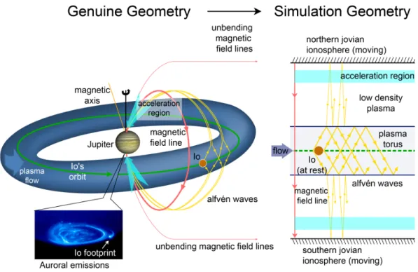
Figure 1.1:Schematic view of the Io-Jupiter interaction in actual geometry (left) and in the rectified geometry applied in our numeric implementation (right).

In the Io-Jupiter scenario, the currents are transmitted via Alfv´en waves that on their way to Jupiter’s polar regions eventually leave the dense medium of the plasma torus. Like other waves, they are partly reflected at interfaces between different propagation mediums. Hence the perturbation partly returns into the torus and further disturbs the plasma in Io’s corotational wake. Downstream of Io a complicated pattern of reflected waves forms, which are able to partly escape the torus and leave eventually an imprint in the Jovian aurora. This is manifested by an extended tail emission structure that trails the main auroral spot and comprises multiple luminosity maxima which are the counterparts of the reflections. In this sense the auroral pattern represents the ”screen” for the magnetospheric wave sequence.

The comparison of the Jovian ionospheric response with a screen is apt also in another sense. In fact, the auroral emissions on Jupiter are generally not excited directly by the Alfv´en waves themselves but the waves accelerate electrons that eventually precipitate into the ionosphere. This takes place in the auroral acceleration region (AAR) close to Jupiter. The beam of accelerated highly energetic electrons that causes luminous effects on the ionospheric ”screen” is to some extent reminis- cent of the layout of a Braun tube or cathode ray tube (CRT) as used in many old monitors and TVs. Apart from electrons that are beamed directly down into the Jovian Ionosphere, some electrons are also accelerated upward. These beams pen-

(19)

5

etrate the equatorial plane close to Io and continue to the conjugate hemisphere, where they cause likewise auroral emissions separated by a few degrees from the main auroral spot.

Observation campaigns of Jupiter’s UV aurora by theHubble Space Telescope(HST) revealed notable variation of the footprint morphology such as the spacing between the different footprints, but also the number of observed emission maxima downstream in the tail. Partly these changes can be attributed to a tilt of the torus central plane with respect to Io’s orbital plane (see Figure 1.1). This inclination causes Io to move up and down in the plasma torus and thus the reflection geometry changes as the distances to the reflecting interfaces varies. Yet, this concept cannot account for all variations observed in the spot pattern. It is known that the interaction strength varies when Io moves from the torus center to the edges, as the impinging plasma density changes from dense to dilute. This has also implications for reflection pattern and the footprint morphology. Finally, apart from reflections that occur at the torus boundaries, the ionosphere and the acceleration region represent additional reflectors. The result of all these superimposed wave reflections that interact and interfere is a complicated pattern which furthermore fluctuates with Io’s position in the plasma torus. Our aim is to increase the understanding of the processes that influence this pattern.

Analytical theory has been successfully applied to describe certain aspects of the wave pattern and the interaction. The global description including all plasma regimes, all reflectors and moreover the interrelation between different reflections is not accessible with analytical methods. Therefore we chose a numerical approach to investigate the electromagnetic coupling between Io and Jupiter.

We use a three-dimensional single fluid magnetohydrodynamical (MHD) model to describe the wave generation, propagation, reflections and wave-wave interactions. Figure 1.1 illustrates how the genuine interaction geometry is converted to our numerical realization. Our simulation geometry is idealized in the sense that we use straight, unbended magnetic field lines (see right part of Figure 1.1). In this configuration, the northern and southern Jovian ionosphere is located at the top and bottom of the simulation box, respectively. The other plasma regimes like the dense torus plasma and the low density plasma population between torus and ionosphere are arranged in layers in our numerical implementation. The AAR is represented likewise by a layer located between torus and ionosphere. As we investigate the interaction in Io’s rest frame, the whole density profile is moving from left to right, while Io stays at rest. The resulting wave pattern evolves downstream, i.e. right of Io.

The application of our model is manifold. First we study the influence of the interaction strength on the footprint morphology. Moreover we infer the location of trans-hemispheric electron beams in the equatorial plane near Io. We trace these beams also further to the conjugate hemisphere and determine the location of the resulting auroral spot. Recently, an interrelation similar to the one we observe between Io and Jupiter was reported to occur between Enceladus and Saturn. Hence we also apply our model to this interaction scenario and discuss the differences.

This brief outline of the Io-Jupiter interaction (or Enceladus-Saturn interaction) and our numerical implementation is intended to provide a rough background. We will revisit the different aspects in detail in the remainder of this dissertation.

(20)

6 Introduction

• In Part I we introduce Io and its plasma and magnetic surroundings. We divide the interaction into sub areas and discuss each against the background of observations and previous models. We process Enceladus similarly but more briefly in chapter two.

• Part II includes the model description after introducing the theoretical framework it is founded on.

• Part IIIcontains our results and a detailed discussion. Furthermore, we qualitatively compare to observational data by theGalileoandCassinispacecrafts as well as to HST findings.

(21)

Chapter 2

Io: Observations and Previous Models

2.1 Io in the Spotlight

The first historical document that mentions Io (not explicitly under that name) is a letter by Galileo Galilei dated January 7, 1610. He reports his observation of three

”stars” near Jupiter. (He discovered the fourth Galilean moon some months later).

Figure 2.1 shows a comparison of the four Galilean moons. Subsequent studies determined the orbital periods of the satellites and Pierre-Simon Laplace revealed the orbital resonance (1:2:4) between Io, Europa and Ganymede in 1788.

In this century, the detection of Jupiter’s radio emissions by Burke and Franklin [1955] was a scientific sensation. Subsequent investigation of the signal’s polar- ization properties proved that the Earth was not the only planet with an intrinsic magnetic field. An Australian meteorologist further discovered the strong correlation between the periodicity of some of the radio burst and Io’s orbital position [Bigg, 1964] suggesting an electromagnetic coupling between the satellite and the planet, a phenomenon which had not been observed before. These findings boosted Jupiter’s attractiveness for space missions and thus withPioneer10 andPioneer11 the first space probes visited the gas giant in 1973 and 1974, respectively. They provided further insight into Io’s interaction with Jupiter and gave first hints of Io’s atmosphere [Kliore et al., 1975]. Moreover the Pioneer findings revealed the high degree of diversity among the Galilean moons. The pictoral idea arose that Jupiter and its satellites represent a ”miniature solar system”. Hitherto, eight space probes visited Jupiter and scientists have learnt a lot about the electromagnetic coupling between the satellites and Jupiter.

On the other hand, major progress in this field can be attributed to the systematic observation of Jupiter’s aurorae e.g. by the HST. Ultraviolet and infrared Emissions emerging from the footprints of the Galilean moons were detected of which the Io footprint is the most intense. Caused by high energy particles precipitating into the atmosphere, aurorae are thought to represent the signature of magnetospheric processes. In this sense, Io’s auroral footprint comprises valuable information about

(22)

8 Io: Observations and Previous Models

the interaction itself. Recent studies suggest that Enceladus is electrodynamically connected to Saturn in a similar way [Pryor et al., 2011]. Even outside our solar system there are strong hints that Alfv´enic coupling possibly takes place between extrasolar planets and their parent stars [Shkolnik et al., 2003; 2005, e.g]. Hence, electrodynamic interplay between two celestial bodies may be common in the universe.

However, Io’s interaction in particular remains an outstanding prime example for ongoing science and also for the present thesis for several reasons. First of all,

Figure 2.1: The four Galilean moons. The top two rows display global views, one with cut-away views showing current concepts of the interiors. The bottom views show how the surface changes as we zoom in on selected features at progressively higher resolution.

Each row down represents an increase in resolution of roughly a factor of ten: the first two rows are at 10 kilometers resolution, increasing to 1 kilometer, 100 meters, and finally 10 meters (bottom). What stands out is the diversity of features at different scales and on the different satellites. [after Schenk, 2010]

(23)

2.2 Jupiter’s Magnetosphere 9

the target is relatively close, and the electromagnetic interaction is the most intense in our solar system. The effects are therefore well observable from Earth.

Sending probes and collecting in-situ data is possible and has already been done.

Moreover, the unique interaction geometry results in a varying strength of the interaction which allows the investigation of a broad range of possible interaction scenarios. Furthermore as we will see in section 2.6.1, the transition of the Alfv´en waves between different plasma regimes causes reflections - a very interesting subject and the main topics of the present work. These reflections leave an imprint in the Jovian aurora as well and thus can be remotely sensed by earthbound observations. For these reasons it is not surprising that an extensive data set of Io footprint surveys and Jovian aurora observations was produced during several HST campaigns. The comprehensive database of remote and in-situ observations allows the comparison of numerical simulation results with measurements and thus provides valuable constraints.

2.2 Jupiter’s Magnetosphere

The observations of radio emissions by Burke and Franklin [1955] cannot only be regarded as a basis for the evidence that Jupiter possesses an intrinsic magnetic field and a magnetosphere, but also provided a means to determine Jupiter’s rotation rate. As the gaseous visible surface rotates differentially, it was cumbersome to find an exact rotation period via cloud tracking. However, in absence of alter- natives, the first Jovigraphic reference systems called System I and System II were founded on this method. After the detection of Jupiter’s radio pulses, the periodicity in the radio signal was considered to reflect the rotation of the Jovian magnetic field and thus its interior [Shain, 1955]. The resulting coordinate system is called System III. In the present thesis we will use this system when referring to Jovi- graphic coordinates and we denote the longitude byλIII. The definition is given in appendix 8.1.

The next major progress in the exploration of Jupiter’s magnetosphere was made particularly by space probe in-situ measurements. ThePioneerandVoyagerobser- vations exposed two significant differences to the Earth’s magnetosphere. First of all they discovered the enormous strength of Jupiter’s internal dipole. With a magnetic moment of∼1.5×10²⁰ Tm³ it is about 18,000 times larger than the terrestrial value. The strong magnetic field forces the plasma in the inner magnetosphere to fully corotate with the planet. Hence, large parts of the magnetosphere are strongly dominated by the Jovian rotation. Moreover, unlike at Earth, Jupiter’s magnetosphere is not populated with primarily heliogenic plasma. The Galilean moons, especially Io, represent the main source of plasma in the magnetosphere. Overall, in Jupiter’s magnetosphere internal sources of energy and plasma are much more important than at Earth, where the solar wind is the dominating factor.

After the visits of thePioneer andVoyager probes, theUlysses spacecraft carried out a swing-by maneuver at the gas giant. While the first two probes mainly provided in-situ measurements near the the equatorial plane, the latter traveled through the Jovian magnetosphere from north to south and yielded rare data from high latitudes. Still, all of these campaigns performed only short-term observations during their flybys. TheGalileo mission reached the Jovian system in 1995

(24)

Figure 2.2:A Schematic view of the Jovian magnetosphere [Khurana et al., 2004]. (Dimen- sions are not to scale)

and provided eight years of long-term observations and also included some high- inclination orbits. However, measurements of a single spacecraft cannot distinguish between spacial and temporal changes in the magnetic field. Thus, the available magnetic field models are still imperfect. The current understanding is as follows: Jupiter’s magnetic field can be approximated by a dipole that is tilted by 9.6^◦against the rotational axis towardsλIII = 202^◦. Additionally, there is a slight offset of the dipole by∼0.13 RJ towardsλ_III = 148^◦andΘ_R=−6^◦(see Figure 8.2 in appendix 8.1 for an illustration and coordinate definitions). However this is just an approximation, as besides the dipole moment there is a substantial contribution of higher order magnetic field terms. Connerney et al.[1982] developed a magnetic field model calledO6, with Gauss coefficients up to sixth order on the basis ofVoy- ager1 data. However, due to large errors, only coefficients up to third order are reliable. Higher order constituents decay faster with distance and as space probes keep a safety distance to Jupiter to avoid high radiation environment, the measure- ment of short wavelength spherical harmonics is only possible with large errors.

A means to remotely sense the surface magnetic field topology is to analyze the track of the auroral footprints of the Galilean moons. This technique has been applied byConnerney et al.[1998] who constructed theVIP4 model in a way such that the observed Io footprints map to the radial distance of the satellite. This model is best suitable for our work, as it further reduces errors especially at Io’s orbital distance and it is most commonly used. However, it has not been optimized by footprint mapping in the azimuthal direction and thus still might contain errors in the longitudinal sense. Recent efforts to improve the surface and small wavelength magnetic field model by introducing a local interior anomaly have been made by Grodent et al.[2008]. The authors improve the predicted latitudinal mapping of all visible Galilean moon footprints in the aurora. However, the benefit for Io is least among the Galilean moons and Io’s predicted footprint track does only slightly dif- fer fromVIP4 based predictions (cf. Figure 2.13). Moreover, unlike other magnetic models, their method introduces an additional shallow and weaker dipole instead

(25)

2.3 Volcanism and Atmosphere 11

of spherical harmonic decomposition up to high orders. Most importantly, it would hamper comparability of our results with those based on the wide-spreadVIP4. We thus use to theVIP4 magnetic field model in the present thesis.

In the middle magnetosphere there is a non-negligible contribution to the magnetic field of the current sheet. Nevertheless, a model byKhurana [1997] that includes this magnetic constituent and also recent calculations of the field fluctuations at Io bySeufert et al.[2011] predict minor influence for regions as close to Jupiter as Io’s orbit. In this area, the internal Jovian field dominates. Hence, we do not discuss the outer and middle parts of the Jovian magnetosphere here and refer the interested reader to the review paper byKhurana et al.[2004].

2.3 Volcanism and Atmosphere

Even before the detection of Io’s volcanic activity, earthbound observations of a neutral sodium (Na) line near Io byBrown and Chaffee[1974] and the detection of a sodium ionosphere byPioneer10 radio occultations [Kliore et al., 1975] led to spec- ulations about the existence of an atmosphere on Io. Evidence for an ionized sulfur component in the Jovian magnetosphere byKupo et al.[1976] were also interpreted as hints for an Ionian atmosphere as it was soon confirmed that the observed material had escaped from Io. Voyager later observed an SO2 absorption profile in the IR band [Pearl et al., 1979] caused by a volcanic plume, indicating a possible source for the atmosphere. Subsequent observations confirmed SO2as main atmospheric species with minor other constituents like sulfur monoxide (SO), sodium chloride (NaCl), and atomic sulfur and oxygen [e.g.Lellouch et al., 2007, and references therein].

Figure 2.3:Picture of an active volcano on Io taken by the Galileo spacecraft. [source: NASA/JPL]

Shortly before the Voyager probes flew through the Jupiter system in 1979, Peale et al.

[1979] predicted volcanic activity on Io. Voyager1 confirmed this presumption by a series of spectacular pho- tos of Io’s active volcanoes [Smith et al., 1979b; Morabito et al., 1979; Smith et al., 1979a].

During the eight years of the Galileo cruise phase at Jupiter, Io and its volcanic activity have been extensively studied (Figure 2.3). More than 100 active volcanoes have been identified - partly effusive, partly eruptive. For a detailed summary of the numerous observations and conclusions we refer the reader to reviews by Williams and Howell [2007] and Geissler and Goldstein [2007]. The fact that the Galileoepoch was not exceptional but Io’s volcanic activity persists was proved by recent images taken by theLong-Range Reconnaissance Imager (LORRI) on-board

(26)

theNew Horizonsspacecraft. They revealed a major eruption of the Tvashtar volcano in the north polar region of Io [Spencer et al., 2007] with an enormous plume.

After several earthbound observation campaigns and the insights given byGalileo (see review byMcGrath et al. [2004]), the current understanding is that Io’s atmosphere consists of a patchy component localized at active volcanoes and a second, more homogeneous distribution generated by surface sublimation of volcanic de- posits and frosts. To what extent both constituents contribute to the atmospheric density is still under debate. Saur and Strobel[2005] use observations of Io’s atmosphere in eclipse, i.e. in absence of sublimation, and derive a minor role of the direct volcanic component (<10%) for the global atmosphere. Conversely Zhang et al. [2003; 2004] successfully reproduce the local atmospheric density structure over volcanic plumes solely with a plume density model which favors partly the volcanic atmosphere concept. A current comparison of numerical results with new observations of Io’s aurora in eclipse byRoth et al.[2011] yields also a minor contribution of volcanoes and supports the hypothesis bySaur and Strobel[2005]. For more detailed background information and discussion the reader is referred to reviews byLellouch et al.[2007] andMcGrath et al.[2004] and references therein.

2.4 Properties of the Ambient Plasma Flow

Before spacecraft missions targeted the giant gas planet, knowledge about the con- tents of Jupiter magnetosphere was limited. Based on findings obtained at Earth, it was believed to be filled with tenuous Heliogenic plasma [e.g.Warwick and Dulk, 1964]. However, earthbound observations provided first evidence for a substantial heavy sulfur plasma component in the inner Jovian magnetosphere [Kupo et al., 1976], whichBroadfoot et al.[1979] later identified as a dense plasma torus around Io’s orbit using theVoyager1 ultraviolet spectrometer (UVS) data.

Along with these remote sensing techniques, in-situ measurements by the Plasma Science (PLS) instrument on-boardVoyagerprovided better spatial resolution and further insight [Bridge et al., 1979]. Based on the data collected byVoyager,Bage- nal[1994] developed an empirical density model by solving multi species diffusive equilibrium equations. Reanalysis of UVS and PLS instrument data provide the basis of this approach as the knowledge of the plasma properties is crucial for this method. More recentGalileo measurements have basically confirmed this model [Frank and Paterson, 2004]. However, Ulysses observations [Hoang et al., 1993] in- dicate a substantially different latitudinal electron temperature profile which leads to a plasma density model with a steeper gradient at the torus edges [Moncuquet et al., 2002]. In all density models, the torus’ central plane is inclined against Io’s orbital plane. The explanation of this phenomenon lies in the magnetic axis tilt of

∼9.6^◦ with respect to the rotational axis (Figure 2.4). The plasma is believed to be generally confined to a magnetic field line. Consequently centrifugal forces drive the plasma towards the point on the specific field line that is farthest away from the rotation axis. All of these points together define a plane called the centrifugal equator (Figure 8.2). It represents the symmetry plane for the latitudinal torus structure and is tilted by∼6.4^◦ against the rotational equator. Due to this tilt, Io moves up and down in the plasma torus on its orbit, periodically approaching the northern and the southern edge of this dense plasma ring (Figure 2.4).

(27)

2.4 Properties of the Ambient Plasma Flow 13

Physical property Symbol [unit] av. value (min-max) Jovian magnetic field (max) B₀[nT] 1720 (2080)

Electron density ne[cm⁻³] 2500 (1200-3800)

Mean ion charge number Z_i[e] 1.3

Mean Ion mass number A_i [amu] 22

Ion Mass density ρ[amu cm⁻³] 42300 (18000-64300)

Ion temperature k_BT_i[eV] 70 (20-90)

Electron temperature k_BT_e[eV] 6

Thermal plasma pressure pi,th[nPa] 22 (3-42) Energetic plasma pressure pi,en [nPa] 10

Total pressure p[nPa] 34

Magnetic pressure B²₀/2µ0[nPa] 1200

Ram pressure ρV²₀ [nPa] 230

Local corotation velocity Vcorot[km/s] 74 Satellite orbit velocity VIo[km/s] 17 Relative plasma velocity V0[km/s] 57

Alfv´en speed VA[km/s] 180 (150-340 )

Sound speed cs[km/s] 29

Alfv´en Mach number M_A 0.31 (0.16-0.39)

Sonic Mach number M_S 2.0 (1.0-2.1)

Fast magnetosonic Mach number MF 0.31 (0.16-0.38)

Alfv´en angle θ_A[^◦] 17 (9-21)

Plasma beta β ∼0.32

Alfv´en conductance ΣA[S] 4.4 (2.4-5.4)

Pedersen conductance Σ_P [S] ∼200

Hall conductance Σ_H [S] 100-200

Electron plasma frequency fpe[kHz] 450 (310-550) Ion plasma frequency fpi[Hz] 2500 (1900-5700) Electron cyclotron frequency f_ce[kHz] ∼48

Ion cyclotron frequency fci[Hz] ∼1.5

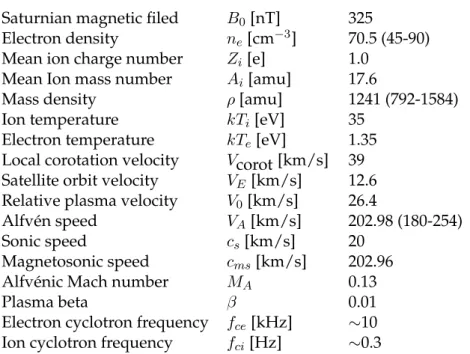
Table 2.1:Physical parameters of the magnetoplasma in the Io torus [Kivelson et al., 2004, and references therein].

The plasma torus rotates with the planets rotation period of 9h 55m 29s which cor- responds to∼74 km/s on Io’s orbit. Io revolves prograde around Jupiter in 42h 27m 33s, giving an orbital velocity of∼17 km/s. This yields a relative velocity of∼57 km/s for the incoming plasma and a period of 12h 57m 10s for one oscillation of Io in the torus. Consequently, Io is exposed to constantly changing plasma conditions depending on its centrifugal latitude.

After the discovery of the torus it has been systematically observed by many scientists who discovered substantial temporal and azimuthal variabilities [e.g.Thomas, 1993, and references therein]. A recent publication bySteffl et al.[2006] using Cassini spacecrafts Ultraviolet Imaging Spectrograph (UVIS) data infers variations of±5%

in the torus density. They are correlated with System III longitude with the maximum at 170^◦. These results are obtained by long-term stacking of the measure-

(28)

Figure 2.4: Sketch of the Io plasma torus and neutral clouds. Left: view fromλIII=292^◦. ω marks the rotation axis. The vertical line represents the rotational equator. M denotes the magnetic axis tilted by ∼9.6^◦ against the rotational axis. The magnetic equator is perpendicular to M. The torus symmetry plane (centrifugal equator, not displayed) inclined by 6.4^◦ with respect to rotational equator. Right: Look down on Jovian north pole. Black dots represent neutrals of different species. Grey circle represents the plasma torus. [after Thomas et al., 2004]

ments as they contain considerable scattering of the data due to much larger temporal variations. Moreover, there is strong observational evidence that the torus structure also varies with local-time (see review byThomas et al.[2004] for details).

Overall, the Io plasma torus properties remain highly transient and, though extensively studied, not fully understood. Yet, a publication currently in press bySmyth et al.[2011] presents a four dimensional (three spatial dimensions and local time) empirical torus model that reproduces torus observations for various epochs and thus might be the basis for a better future comprehension.

2.5 Io’s Local Interaction: The Generator

Io’s interrelation with the Jovian magnetosphere has been of substantial interest ever sinceBigg[1964] discovered the correlation of Jupiter’s decametric radio emission (DAM) and Io’s orbital position. An accurate description of the interaction requires both, detailed knowledge of the obstacle properties and the characteristics of the incoming magnetoplasma. As we outlined these two factors in the previous sections, we now turn to the interaction itself.

In a simplified electrostatic image, the interaction can be divided into three parts:

the generator, the load and the coupling region. We describe the generator region in this paragraph and will subsequently elucidate the observations and models available for the load in the system where the energy is dissipated: Io’s footprints in the Jovian aurora and the radio emissions.

(29)

2.5 Io’s Local Interaction: The Generator 15

Most of the theoretical concepts of Io’s local interaction that have been developed to explain this electrodynamic interaction employ the framework of magnetohydro- dynamics (MHD), which is a convenient albeit not complete description. Within the ideal MHD theory, three wave modes exist. Two of them are compressional modes called slow and fast magnetosonic waves. The third mode is a transverse mode with the outstanding ability to carry electric currents almost lossless parallel to the ambient magnetic field. This mode is essential for the coupling of Io to the Jovian ionosphere and to interconnect magnetospheric processes and ionospheric response.

The description of the plasma as a fluid is legitimate when the characteristic macro- scopic length and time scales (i.e. Io’s radius and plasma convection time) are much larger than their microscopic counterparts (i.e. the ion gyro radii and periods). The characteristic plasma parameters at Io are presented in Table 2.1. One can see that the conditions for the fluid approximation are well fulfilled.

We note that some important aspects of the interaction take place on smaller scales.

However, the focus of this work is put on the far field MHD wave pattern and related phenomena and not on the precise description of the Alfv´en wave generator region on all scales. For the aim of our study the fluid approach provides the required precision whilst reducing complexity.

It is notable that within the continuum description, two rival paradigms exist.

Some models favor the formulation with the electric fieldEand the current density jas fundamental variables, others use the magnetic fieldB and bulk velocitiesv as principle quantities. The pros and cons of both paradigms are discussed and weighted for instance byVasyli ¯unas [2001; 2005]. Yet, there is an ongoing discussion about which is the best formulation. However, since both theories have been successfully applied to describe different aspects of the Io-Jupiter interaction we will make use of both concepts to explain the physics of the interaction whichever is more intuitive. In the following paragraphs we will discuss the different models that have been developed to characterize the interaction.

2.5.1 The Unipolar Inductor Model

While Io orbits Jupiter, it is continually overtaken by the corotating magnetospheric plasma linked to the Jovian magnetic field. In the satellites rest frame the relative motionV0with respect to the rotating magnetic fieldB0creates a motional electric field

E₀=−V₀×B₀ . (2.1)

It is roughly directed radially away from Jupiter (Figure 2.5). While in most space plasmas conductivity is generally high along the magnetic field direction, it is small in the perpendicular plane. A way to short-circuit the electric field is a potent conductor. Early concepts of the interaction byPiddington and Drake[1968] andGoldre- ich and Lynden-Bell[1969] hence assume Io’s surface to be highly or even infinitely conductive, so that the motional eclectic field can drive currents in the surface layer.

AsGoldreich and Lynden-Bell[1969] also assume infinite conductivity along the magnetic field direction, these currents can continue along the magnetic field and close in the Jovian ionosphere. The result is a current circuit as depicted in Figure 2.5.

The assumption of a perfectly conductor Io implies that the magnetospheric cur-

(30)

Figure 2.5:The current loop model: Io as unipolar inductor. Magnetic field lines are plotted in black. Red arrows represent electric currents.

rents are confined to the surface of the magnetic flux tube connected to Io. The interior of the flux tube is force-free in Io’s rest frame, hence it is rigidly attached to Io. It is therefore termed Io flux tube (IFT). The current system thus forms a steady loop in which Io acts as a unipolar inductor. Consequently this model is called current loop model

Figure 2.6: Current loop or unipolar inductor setup.

Left: side view; Right: front view. Currents are strictly field aligned. [after Saur et al., 2004]

In this setup, the currents flow- ing between Io and Jupiter are carried by Alfvén waves. The authors note that their model is only valid, if the Alfvén waves reflected at the Jovian Iono- sphere are able to reach Io before it has moved away. In other words, they require the round-trip travel timeτ_Aof the Alfvén mode to be small compared to the convection timetc

of the plasma past Io:

τ_A

t_c 1. (2.2) Goldreich and Lynden-Bell[1969] assumed a low density plasma in the Jovian magnetosphere. This implies a high Alfv´en wave velocityVAwhich is given by

V_A= B

√µ₀ρ , (2.3)

whereρrepresents the plasma mass density andµ₀the vacuum permeability. Con- sequently, the authors hypothesize that the required travel time ratio (2.2) would be easily fulfilled. This assumption was reasonable at the time. However, it became arguable with the detection of the dense plasma torus.

(31)

2.5 Io’s Local Interaction: The Generator 17

The current loop model also assumes that the currents which couple Io to Jupiter are strictly field aligned [e.g.Piddington and Drake, 1968]. This approach neglects plasma inertia. As Io’s conductance short circuits the motional electric field, the currents that are partly compensating the charge separation between the Jupiter facing and the anti-Jupiter hemisphere perturb the original electric field. This implies acceleration or deceleration of the surrounding plasma. These acceleration terms must be compensated byJ×Bforces [Neubauer, 1980]. This component of the current system perpendicular to B gains relative importance with increasing plasma momentum and thus with the mass density of the incoming plasma. Since the quantity ofρalso affects the Alfv´en velocity (2.3), one can assess the significance of plasma inertia by the Alfv´en Mach number

M_A= V0

VA

. (2.4)

The detection of the dense plasma torus put new constraints on the local Alfvén Mach number on Io’s orbit and the restriction to strictly field aligned currents is hardly maintainable. Moreover, with the observation of Io’s ionosphere, Io’s surface conductivity needed to be replaced by typical ionospheric Hall and Pedersen conductivities. This questions the assumption of a force-free Io flux tube and thus a rigid connection of the IFT plasma to Io. Hence two major aspects challenge the current loop model. First, the convection time of the plasma past Io is smaller than initially believed since the IFT is not force-free and a non-zero plasma velocity remains. Secondly, the Alfvénic travel time is larger than believed, due to the dense torus plasma that slows down propagation of Alfvén waves. Hence condition (2.2) is not always fulfilled and the validity of the model is questionable.

The new observations triggered the development of new models, such as the Alfv´en wing model which we present in the next paragraph.

2.5.2 The Alfv´en Wing Model

Figure 2.7:Side and front view of the Alfv´en wing model [Neubauer, 1980]. Currents flow along the Alfv´en characteristics and are closed at far distances (not shown).

Goertz and Deift[1973] discuss certain aspects of the effects of a weaker Io-Jupiter

(32)

interaction as it is the case for a low conducting Io. A model byDrell et al.[1965]

studies Alfv´enic perturbations that were observed to decelerate the satelliteECHO at Earth. However, they consider small perturbations only and thus justify a lin- earization of the equations and disregard second order terms.

Neubauer[1980] developed the first consistent theoretical framework of the standing Alfv´enic current system. It is valid for weak and strong interaction settings.

It is a fully nonlinear treatment of the problem and valid for an isotropic plasma.

However, it is intended to be applied for the current system at some distance of Io, not for the direct interaction region, as e.g. compressional modes cause plasma anisotropy. To some extent contrary to the current-loop approach, the author finds that the currents flow along the Alfv´en characteristics . They are defined as:

C^±_A : V^±_A =V±V_A=V± B

√µ0ρ (2.5)

and prescribe the propagation direction of Alfv´en waves with respect to Io (Vrep- resents the plasma bulk velocity field in Io’s rest frame). The waves generated at Io propagate away in theC^±_A-directions and form a wing-like structure (see Figure 2.7). Thus the currents are not strictly field-aligned.

However, when the plasma is at rest inside the magnetic flux tube connected to Io, i.e. for a saturated interaction as considered in the current loop model, the propagation is strictly field aligned (Figure 2.6). In this case the magnetic field direction and the Alfv´en characteristics coincide.

The Alfv´en wing model represents the basis for the work at hand and because of its importance we revisit this model in section 4.2 of this work.

2.5.3 Other Models

As the enigma of Io’s interaction attracted considerable attention, many theories and models have been published. Because of the complexity but also due to numerical difficulties and limited computational resources, different groups have focused on particular aspects of the problem. We will try to extract the most influential ones and give a very brief summary of the major aspects.

Deift and Goertz[1973] consider an inhomogeneous plasma density, but solve the wave equations linearly. However, they predict reflections and discuss wave-wave interaction (see subsequent section). Other models include pickup processes for current closure in Io’s vicinity [Goertz, 1980] or in its corotational wake [Southwood and Dunlop, 1984].

Saur et al.[1999] focused on the local interaction properties and addressed the problem in a stationary, 3D, two fluid model including aeronomic processes and a detailed description of the ionosphere (involving ion production rates and collision frequencies). They find that the resulting anisotropic electric conductivity distribution has important effects on the local interaction. Most importantly, the authors realize for the first time the importance of the Hall effect in Io’s close vicinity. It significantly rotates the motional electric field in the satellites ionosphere. Dols et al.

[2008] include a more detailed description of Io’s atmospheric chemistry and focus on a multi-species description of the local interaction. They stress the possibility of

(33)

2.6 The Far Field Interaction: The Coupling 19

an enhanced ionospheric conductivity caused by precipitating energetic electrons associated with observed equatorial electron beams.

With increasing computer power, numerical approaches to describe the Io interaction became possible. Wolf-Gladrow et al. [1987] published one of the first 3D models. It calculates self-consistently electric field, electric current and magnetic field data. Meanwhile Linker et al.[1988; 1989; 1991] also developed a 3D model using a single fluid resistive MHD approach and thus also included compressional MHD wave modes. However, they focus on the local interaction only. Kopp[1996]

use their 3D resistive MHD code with implemented mass loading to qualitatively deduce plasma production rates. They also find in their data a current system in Io’s wake, thus confirming the results ofSouthwood and Dunlop[1984]. Combi et al.

[1998] also apply an ideal single fluid MHD code, but with a very good spatial resolution owing to adaptive mesh refinement. They successfully reproduce single features of data collected on theGalileoI0 flyby.

2.6 The Far Field Interaction: The Coupling

The coupling region between Io, the generator, and the load in Jupiter’s polar regions is a large and heterogeneous area. Along the travel path of the generated waves, the propagation medium and the ambient magnetic field vary significantly.

On the one hand this implies wave reflections and interference, on the other hand kinetic effects gain importance in low-density areas located at high magnetic latitudes. We classify these phenomena as far-field interaction and outline the associated physical effects in this section.

2.6.1 Alfv´en Wave Propagation and Reflections

When Alfv´en waves generated in Io’s vicinity eventually reach the edge of the plasma torus (Figure 2.8), the wave velocity changes due to the plasma density gradient (2.3) and the wave is partially reflected as illustrated in Figures 2.8 and 2.9. The strongest observational evidence for this phenomenon is given by multiple emission maxima detected in the auroral tail emission by HST [Connerney and Satoh, 2000] and sets of DAM arcs in the time-frequency spectra of Jupiter’s radio emissions. The subject of reflections was addressed analytically and numeri- cally before and very different results have been found by different authors.Goertz [1980] calculates the reflection coefficient for a constant magnetic field and con- cludes, in contrast toNeubauer[1980], that torus-internal reflections are negligible.

Subsequent 1D numerical studies byWright[1987] andWright and Schwartz[1989]

investigate the reflection of Alfv´en waves with updated torus density profiles and an additional magnetic field gradient and derive a reflection coefficient of 50%. A one-dimensional MHD model byDols[2001] indicates that only 40% of the Alfv´en wave energy is able to leave the torus. In a 2D MHD modelDelamere et al.[2003]

observe that only 20% energy can escape the torus. Su et al.[2006] use a gyro-fluid model and infer likewise a reflection intensity of∼80%. These models give essen- tially different results which can be mainly attributed to the model and the use of different density profiles. Uncertainties in the magnetic field model and the absence of measured plasma density profiles along the magnetic field lines (not to

(34)

Figure 2.8: Io is embedded in the dense corotating torus. The motion of the plasma relative to the satellite generates Alfv´en waves that are partly reflected at the torus edges and Jupiter’s ionosphere.

mention the spatial and temporal variability of the density) hampers the quantita- tive assessment of the reflection coefficient.

Besides the amplitude of wave reflections, the resulting wave pattern in the wake region downstream of the obstacle and the initial Alfvén wing is of particular interest. In the pure Alfvén wing approach, the angle of incidence equals the angle of reflection [e.gSaur et al., 2004], the resulting wave field looks as depicted in the top panel of Figure 2.9. This holds only for a weak interaction, when the magnetic field and velocity perturbations are small. Strong interactions greatly modify the Alfvén characteristics which determine the travel path of incoming wave and wave reflection. The consequence is a breakdown of the regular reflection law [Jacobsen, 2006;Jacobsen et al., 2007] as illustrated in the lower panel of Figure 2.9. In extreme cases the reflection follows the travel path of the incoming wave back to the Alfvén wave generator. This scenario can be described with the unipolar inductor model.

Hence, this framework represents a special case of the general Alfv´en wing model [Neubauer, 1980].

All models mentioned so far neglect nonlinear effects between the incident and the reflected wave. Yet, they are indispensable for the description of the Io-Jupiter interaction. At the torus boundary, the incoming wave interacts with the reflection and both perturbations superimpose and interfere. Moreover, other wave modes are excited upon reflection, modulating the reflection energy budget and again mu- tually interacting with other waves and wave modes. The question arises to what extent these effects influence the MHD wave pattern. Jacobsen[2006] andJacobsen et al.[2007] address this problem with a 3D MHD model and perform detailed studies with emphasis on the resulting MHD wave pattern depending on the strength of the interaction. They compare the results qualitatively to auroral footprint observations which provide a valuable means to evaluate the findings as they represent

(35)

a two-dimensional cross section through the Alfv´en wave pattern. Additionally, the breakdown of the reflection law can be observed in these simulations. As these results represent the basis for the present study and they are essential for the interpretation of the findings presented here, we reformulate the results in part III of this work.

2.6.2 Acceleration Region

Figure 2.10:Concept of the auroral acceleration region. [after Pilipenko et al., 2004]

Outside the dense plasma torus the number of charge carriers decreases rapidly, whereas the magnetic field strength increases and the cross-section of the current channeling flux-tubes be- comes smaller. Superficially, current maintenance thus demands electron acceleration. This happens where the ion density decreases below a certain threshold value in the region where the maximum Alfv´en velocity is reached [Knight, 1973], the so-called auroral acceleration region (AAR). Figure 2.10 shows a sketch of the acceleration region.

Observational evidence for such phenomena at Jupiter comes from detected short-burst radio emissions near 20 MHz presumably triggered by the acceleration [Zarka, 1998]. The acceleration region is located between an altitude of approximately 0.9 RJ and 2.9 RJ above the ionosphere [Hess et al., 2007;Ray et al., 2009]. The acceleration mechanism has been widely discussed and is still under debate. Concepts like electrostatic double layers [Smith and Goertz, 1978], kinetic or inertial Alfv´en waves [Swift, 2007;Jones and Su, 2008] and repeated Fermi accelerations [Crary and Bagenal, 1997] have been brought up and modeled. These studies were mostly motivated by the interpretation of the planetward electron beams as a source for the aurora. For Earth, Mauk et al.

[2002] distinguish between three types of aurora: (1.) Alfv´en aurorae, and aurorae associated with (2.) upward and (3.) downward current regions. For Jupiter, Su et al.[2003] follow this argumentation and identify the main spot emission as Alfv´en aurora. However, some electrons are also accelerated upward, i.e. in the anti-planetward direction. They have been observed in the equatorial plane near Io and are treated in the next paragraph.

2.6.3 Equatorial Electron Beams

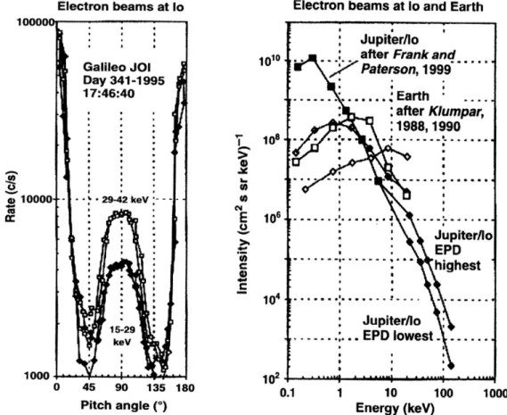
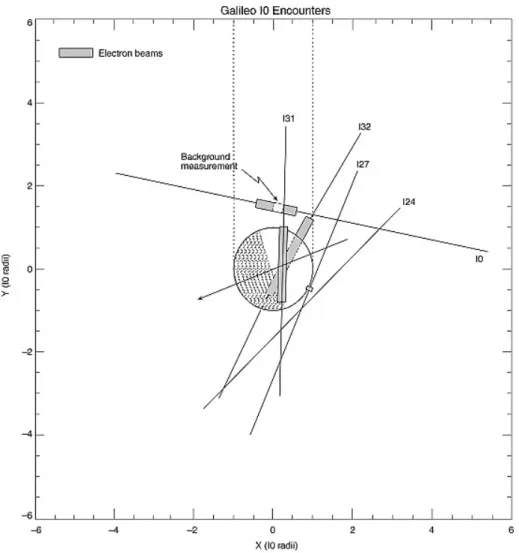
Associated with Io’s interaction with the ambient magnetoplasma, energetic field- aligned electron populations have also been observed in-situ by theGalileo spacecraft near Io.Williams et al.[1996; 1999] andFrank and Paterson[1999] report intense bi-directional electron beams in Io’s wake. Williams and Thorne [2003] and Frank

(36)

Figure 2.9: Schematic view of the Alfv´en characteristics for different interaction scenarios.

Top panel represents a weak interaction. In this case the angle of incidence equals the angle of reflection. The result is a rhombic wave pattern in the downstream direction. Bottom panel depicts the strong interaction scenario. Conversely, a regular law of reflection does not apply here [after Saur et al., 2004].

and Paterson[2002b] detect high-energy electrons streaming onto Io’s poles during

(37)

Figure 2.11: Properties of observed electron beams at Io and at Earth. Left: Pitch angle distribution of electron counts in the different energy channels of the detector for the Galileo I0 flyby. Right: Phase space density spectra of field aligned electron beams. Hollow symbols represent observations at Earth. Filled symbols depict a combination of electron measurements by Galileo [after Mauk et al., 2001].

two polar flybys (I31 and I32). The measured pitch-angle¹ distributions suggest that these electron beams originate at high latitudes close to Jupiter where electrons are accelerated upward (anti-planetward), towards Io. Even though the exact link between the planetward and anti-planetward electron beams at Io is not fully understood, the process of anti-planetward electron beams in association with auroral features appears to be a universal property of aurorae [Saur et al., 2006]. These beams are known to occur close to Io, in the magnetosphere of Earth [Klumpar, 1990;

Carlson et al., 1998], Jupiter [Tom´as et al., 2004;Frank and Paterson, 2002a;Mauk and Saur, 2007] and Saturn [Saur et al., 2006;Mitchell et al., 2009]. The main advantage of studying Io’s auroral footprints and energetic particle populations compared to other solar system auroral features is that the location of the initial source region, i.e. Io’s interaction region, is known and the perturbation is continuous.

The electron beams at Jupiter have first been observed near the equator with the Energetic Particle Detector(EPD) on theGalileospacecraft. In December 1995, during the first Io flyby an energetic field-aligned electron population was measured in Io’s wake [Williams et al., 1996]. The pitch angle distribution was bidirectional. In

1The pitch angle is defined as angle between the particle velocity vector and the magnetic field vector.