Quantum Monte Carlo studies of a metallic spin-density wave transition
Inaugural-Dissertation zur
Erlangung des Doktorgrades
der Mathematisch-Naturwissenschaftlichen Fakultät der Universität zu Köln
vorgelegt von
Max Henner Gerlach
aus Köln
Köln 2017
Prof. Dr. Achim Rosch
Tag der mündlichen Prüfung: 20.01.2017
Abstract
Plenty experimental evidence indicates that quantum critical phenomena give rise to
much of the rich physics observed in strongly correlated itinerant electron systems
such as the high temperature superconductors. A quantum critical point of particular
interest is found at the zero-temperature onset of spin-density wave order in two-
dimensional metals. The appropriate low-energy theory poses an exceptionally hard
problem to analytic theory, therefore the unbiased and controlled numerical approach
pursued in this thesis provides important contributions on the road to comprehensive
understanding. After discussing the phenomenology of quantum criticality, a sign-
problem-free determinantal quantum Monte Carlo approach is introduced and an
extensive toolbox of numerical methods is described in a self-contained way. By
the means of large-scale computer simulations we have solved a lattice realization
of the universal effective theory of interest. The finite-temperature phase diagram,
showing both a quasi-long-range spin-density wave ordered phase and a d-wave
superconducting dome, is discussed in its entirety. Close to the quantum phase
transition we find evidence for unusual scaling of the order parameter correlations
and for non-Fermi liquid behavior at isolated hot spots on the Fermi surface.
Kurzzusammenfassung
Zahlreiche experimentelle Ergebnisse deuten darauf hin, dass quantenkritische
Phänomene der Auslöser für einen Großteil der reichhaltigen Physik sind, die
man in Hochtemperatursupraleitern und anderen stark korrelierten Systemen be-
weglicher Elektronen beobachtet. Ein besonders interessanter quantenkritischer
Punkt findet sich in zweidimensionalen Metallen am Übergang zu antiferromag-
netischer Spindichtewellen-Ordnung am absoluten Temperatur-Nullpunkt. Die
zugehörige Niedrigenergie-Theorie ist mit analytischen, theoretischen Methoden
sehr schwer zu lösen, so dass ein umfassendes Verständnis bisher nicht erreicht
werden konnte. In dieser Dissertation wird als komplementärer Zugang ein nu-
merischer Ansatz verfolgt, mit dem wichtige Beiträge geliefert werden können, weil
alle Rechnungen gut unter Kontrolle zu halten sind und keine händisch gesetzten An-
sätze die Ergebnisse in bestimmte Richtungen drängen. Nach der Besprechung
der Phänomenologie von Quantenkritikalität wird ein vorzeichenproblemfreies
Determinanten-Quanten-Monte-Carlo-Verfahren eingeführt und ein umfassender
Satz numerischer Methoden beschrieben. Dieser Methodenteil kann weitgehend
für sich stehen. Mittels groß angelegter Computersimulationen haben wir eine
Gitterrealisierung der universellen effektiven Theorie dieses Problems gelöst. Das
Phasendiagramm bei endlicher Temperatur beschreiben wir in seiner Gänze. Es
weist sowohl eine quasi-langreichweitig geordnete Spindichtwellen-Phase als auch
eine d-Wellen-supraleitende Phase auf. In der Nähe des Quantenphasenübergangs
können wir Nachweise für ein ungewöhnliches Skalenverhalten der Ordnungsparam-
eterkorrelationen und für fermionische Eigenschaften, die an isolierten Punkten der
Fermi-Fläche nicht den Erwartungen nach Landaus Theorie der Fermi-Flüssigkeiten
entsprechen, finden.
Contents
1 Introduction 1
I Quantum phase transitions and unconventional super-
conductivity 5
2 Modeling quantum phase transitions 7
2.1 Introduction to quantum phase transitions . . . . 7
2.1.1 Phase transitions, criticality, and universality . . . . 7
2.1.2 Interplay of thermal and quantum fluctuations . . . . 9
2.1.3 Scaling at quantum phase transitions . . . 11
2.1.4 Effective theories . . . 12
2.2 Quantum phase transitions in systems of itinerant electrons . . . 14
2.2.1 Motivation of the spin-fermion model . . . 14
2.2.2 Metal close to the onset of spin-density wave order . . . 19
2.2.3 Analytical approaches beyond mean field . . . 21
3 Unconventional superconductivity on the verge of antiferromagnetism 25 II Numerically exact solution by quantum Monte Carlo 29 4 Quantum Monte Carlo approach 31 4.1 Determinantal quantum Monte Carlo (DQMC) . . . 32
4.1.1 Basic formalism . . . 33
4.1.2 Markov chain Monte Carlo sampling . . . 35
4.1.3 Observable expectation values . . . 39
4.2 Fermion sign problem . . . 44
4.2.1 Absence of the sign problem . . . 46
4.2.2 Determinant factorization . . . 47
4.2.3 Generalized time reversal symmetry . . . 50
4.2.4 More sign-problem-free formulations . . . 54
4.3 Sign-problem-free two-flavor model . . . 54
4.3.1 Mean field . . . 56
4.3.2 Single-fermion matrix structure and antiunitary symmetry . . 58
4.3.3 Fermion determinant and O ( N ) symmetric variations . . . 59
4.3.4 Other types of Fermi surfaces . . . 62
5 Numerical methodology 63 5.1 Numerical stabilization . . . 63
5.1.1 Matrix decomposition for the equal-time Green’s function . . 65
5.1.2 Efficient and stable DQMC sweep . . . 68
5.2 Monte Carlo updating schemes . . . 72
5.2.1 Local updates . . . 73
5.2.2 Global updates . . . 79
5.2.3 Replica exchange . . . 82
5.3 Efficient linear algebra . . . 91
5.3.1 Checkerboard break up . . . 91
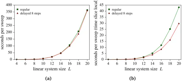
5.3.2 Delayed updates . . . 96
5.4 Finite-size effects . . . 101
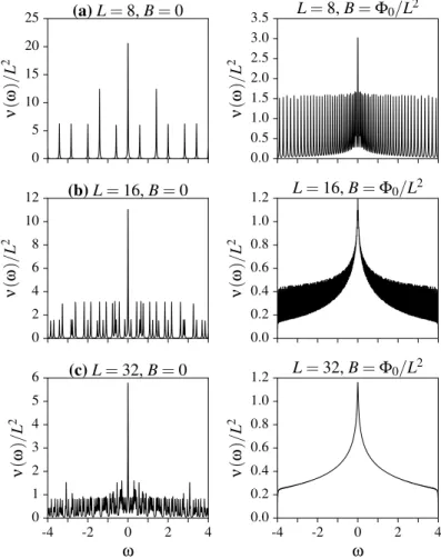
5.4.1 Perpendicular magnetic field . . . 101
5.4.2 Fictitious “magnetic” field for the SDW model . . . 104
5.4.3 Twisted boundary conditions . . . 106
5.5 Aspects of data analysis . . . 107
5.5.1 Multiple histogram reweighting . . . 108
5.5.2 Correlation functions via fast Fourier transform (FFT) . . . 110
III Numerical results 113 6 Phase diagrams and competing orders 115 6.1 Analysis of the spin-density wave (SDW) transition . . . 116
6.2 Phase diagram for λ = 1 = c . . . 119
6.3 Identification of the superconducting transition . . . 120
6.4 Phase diagram for λ = 3, c = 2 . . . 125
6.4.1 Competition and coexistence of magnetic and superconducting order . . . 127
6.4.2 Charge-density wave (CDW) and pair-density wave (PDW) susceptibilities . . . 132
6.5 Phase diagrams for several values of λ and c = 3 . . . 136
6.6 Discussion . . . 139
7 Manifestations of quantum critical behavior 143 7.1 Magnetic correlations . . . 143
7.1.1 Bosonic SDW susceptibility . . . 144
Contents
7.1.2 Fermion bilinear SDW susceptibility . . . 149
7.1.3 Temperature dependence . . . 151
7.2 Single-fermion correlations . . . 155
7.3 Superconducting state . . . 160
7.4 Discussion . . . 162
8 Concluding remarks and outlook 165
A Identities for fermionic many-particle states 169
B Promoting charge-density wave order 175
C Hybrid Monte Carlo 179
Bibliography 183
Acknowledgments 197
1 Introduction
To this day various classes of highly correlated itinerant electron systems such as the high temperature superconductors elude full physical understanding. It is widely believed that the key to the solution of many open problems concerning these materials can be found in quantum critical phenomena, i.e. continuous phase transitions at zero temperature, driven by quantum fluctuations and tuned by a non-thermal control parameter [ 1–3 ] . Quantum phase transitions are particularly hard to reason about in metallic systems, where fermionic quasiparticles at low energies close to the Fermi surface strongly interact with critical order parameter fluctuations [ 4, 5 ] . As a consequence it is often not sufficient to deal with effective theories of an order parameter field alone with the fermions integrated out. A viable approach can rather be found in low energy theories that incorporate both a collective bosonic order parameter and fermions which are free apart from the coupling to the bosons [ 6 ] . Since there are no obvious small parameters, the solution of these theories is very hard by purely analytic approaches.
The topic of this thesis is one important type of metallic quantum phase transitions, namely the transition between an itinerant, but antiferromagnetic spin-density wave (SDW) ordered state and a quantum-disordered paramagnetic state. The magnetic quantum critical point at the zero-temperature boundary between these two phases is believed to be prototypical for the physics of the cuprates, certain iron-based and heavy fermion superconductors, and other materials [7].
We pursue an alternative route to solving a low-energy theory realizing this quantum phase transition that is complementary to analytic theory. Our method of choice is a flavor of quantum Monte Carlo (QMC) adapted to the simulation of coupled fermion-boson many-particle lattice models at finite temperature [ 8 ] . At this time QMC is the only established numerically exact, unbiased method capable of providing solutions for such systems in two spatial dimensions on moderately large lattices in polynomial time. Its applicability is unfortunately limited to models free of the “fermion sign problem” [ 9 ] , which has hindered progress for long, but fortunately a sign-problem-free realization of a metallic SDW model has been found recently [ 10, 11 ] .
This thesis is structured into three parts. In Part I we start with a short introduction
to the phenomenology of quantum phase transitions with a special emphasis put
on the quantum critical regime at finite temperatures above a quantum critical
point. The concept of effective order parameter field theories is discussed with its
shortcomings for systems with Fermi surfaces. The spin-fermion model is carefully
introduced as an adequate model to analyze a metallic spin-density wave quantum phase transition and analytical approaches to its solution are summarized. Three classes of strongly correlated materials at the focus of experimental research are the subject of the subsequent Chapter 3: the cuprates, the iron-based superconductors, and the heavy fermion systems. They have in common that their phase diagrams feature an antiferromagnetic phase in vicinity of an unconventional superconducting phase whose existence can be linked to quantum critical phenomena.
The goal of Part II is to give a mostly self contained account of the numerical methods we have used to study the metallic SDW model. In Chapter 4 the versatile and numerically exact method of determinantal quantum Monte Carlo (DQMC) is introduced in its finite-temperature formulation. The largest limit to its applicability is the fermion sign problem plaguing most simulations of interacting electron sys- tems. Here we show how to circumvent it for our model by moving to a two-band variation, carefully constructed to be symmetric under a generalized time-reversal transformation. The nature of Chapter 5 is very technical. While the aspects of the method that we discuss here may appear to be mere implementation details, their attentive consideration is a prerequisite for obtaining correct numerical results in limited computing time.
Finally, Part III presents the rich physics found in the numerically exact results obtained in the simulations of our variation of the spin-fermion model. Detailed finite-temperature phase diagrams for several sets of parameters are discussed in their entirety in Chapter 6. In the vicinity of an SDW quantum phase transition we do not only find a quasi-long-range ordered SDW phase, but also an emergent d-wave superconducting phase. The susceptibilities of various potentially competing orders are also investigated. Chapter 7 then focuses on manifestations of quantum critical behavior associated with a putative quantum critical point underlying the superconducting phase. At temperatures above T
corder parameter correlations are found to agree surprisingly well to Hertz-Millis theory, but show intriguing deviations in their temperature dependence. Moreover, in an apparently quantum critical regime non-Fermi liquid behavior is induced for momenta close to the “hot spots” of the Fermi surfaces. Here we also give a closer look at properties of the superconducting state close to the quantum phase transition.
We close in Chapter 8 with concluding remarks and an outlook on the prospects of future continuations of this work.
This thesis is the outcome of an intensive collaboration with Yoni Schattner and
Erez Berg of the Weizmann Institute of Science. Two independent software codes
for simulation and evaluation have been used in combination. At the beginning
of Chapsters 6 and 7 it is pointed out which parts have not been evaluated by the
author of this thesis, but have been obtained by the Weizmann group.
The C++ software developed by the author, implementing efficient algorithms for DQMC simulations, is available to the public under the free Mozilla Public License (MPL) version 2.0:
• M. H. Gerlach, maxhgerlach / detqmc: First release of detqmc [data set], Zenodo (2017). http://doi.org/10.5281/zenodo.290197, https://github.com/
maxhgerlach/detqmc .
The results presented in this thesis have been published previously in these papers:
• Y. Schattner, M. H. Gerlach, S. Trebst, and E. Berg, Competing Orders in a Nearly Antiferromagnetic Metal, Phys. Rev. Lett. 117, 097002 (2016).
• M. H. Gerlach, Y. Schattner, E. Berg, and S. Trebst, Quantum critical properties of a metallic spin-density-wave transition, Phys. Rev. B 95, 035124 (2017).
During the time frame of the author’s doctoral research work two additional papers have been published, which are not covered in this thesis:
• E. Sela, H.-C. Jiang, M. H. Gerlach, and S. Trebst, Order-by-disorder and spin- orbital liquids in a distorted Heisenberg-Kitaev model, Phys. Rev. B 90, 035113 (2014).
• M. H. Gerlach and W. Janke, First-order directional ordering transition in the three-dimensional compass model, Phys. Rev. B 91, 045119 (2015).
These address problems of frustrated spin systems, which have been tackled by
extensive classical Monte Carlo simulations. The second of these papers is mainly
based on data obtained during the author’s diploma thesis work.
Part I
Quantum phase transitions and
unconventional superconductivity
2 Modeling quantum phase transitions
Phase transitions are ubiquitous in various complex systems in nature, including the freezing of water, the spontaneous magnetization of a ferromagnetic material, or the transition of a metal into a superconducting state. These example phase transitions all take place at finite temperatures. At the transition temperature a macroscopic type of order is destroyed by thermal fluctuations. Conversely, quantum phase transitions occur at zero temperature, where a control parameter other than temperature such as pressure, chemical composition, or an external field is varied across a transition point.
Only quantum fluctuations, ultimately a manifestation of Heisenberg’s uncertainty principle, destroy order in this case. Even though the third law of thermodynamics precludes experiments at absolute zero, zero temperature quantum critical points (QCPs) have attracted considerable interest in condensed matter physics. The reason for this is that the special excitation spectrum of the ground state at a QCP gives rise to quantum critical behavior also at finite temperatures in a regime above the transition point. This influences physical observables over a wide range of the phase diagram. Understanding quantum criticality is a key objective on the road to uncovering the mechanisms behind phenomena such as high-temperature superconductivity.
In this Chapter, Sec. 2.1 first introduces quantum phase transitions in general, then Sec. 2.2 proceeds to discuss the modeling of quantum phase transitions in systems of itinerant electrons, focusing on a spin-density wave (SDW) transition.
2.1 Introduction to quantum phase transitions
In this Section we briefly introduce the general phenomenology of quantum phase transitions [ 4, 12, 13 ] . The presentation mostly follows M. Vojta’s review [ 12 ] .
2.1.1 Phase transitions, criticality, and universality
Generally, we distinguish between first-order phase transitions and continuous phase
transitions. First-order transitions are characterized by the coexistence of two phases
at the transition point, while phases do not coexist at a continuous transition. A
conventionally ordered phase is described by a local order parameter, which is zero
outside of the ordered phase and takes up a non-unique, non-zero value in the
ordered phase. At the critical point of a continuous transition the value of the order parameter vanishes continuously as it is crossed from the ordered phase.
In the disordered phase the expectation value of the order parameter is zero, but it has non-zero fluctuations. As the critical point is approached, spatial correlations of these fluctuations become long-ranged and the correlation length ξ, which is their typical length scale, diverges as
ξ ∼ | t |
−ν, (2.1)
where ν is the correlation length critical exponent and t measures the distance to the critical point. For a thermal phase transition at a temperature T = T
cone can set t = ( T − T
c)/ T
c. Similarly, there are also long-range correlations of order parameter fluctuations in time. The typical time scale for their decay is the correlation time τ
c, which in the vicinity of the critical point diverges as
τ
c∼ ξ
z∼ | t |
−zν(2.2)
with the dynamical critical exponent z. Close to the critical point, ξ is the only characteristic length scale and τ
cis the only characteristic time scale of the system.
By Eqs. (2.1) and (2.2) correlation length and time are infinite at the transition point. Since there fluctuations occur on all length and time scales, the system must be scale invariant. Consequently, all measurable quantities depend via power laws on the external parameters; one speaks of critical phenomena. Near the critical point the exponents of these power laws, the critical exponents, fully characterize the behavior of the system.
To illustrate the concept of scaling let us consider a classical ferromagnet, where the magnetization M ( r ) is the order parameter and external parameters are the reduced temperature t = ( T − T
c)/ T
cand an applied magnetic field B, which couples to M . Close to the critical point all physical properties must be invariant under rescaling of all lengths in the system by a common factor if we simultaneously adjust the external parameters such that the correlation length, which is the only important length scale, remains unchanged. By requiring this we obtain a homogeneity relation for the singular part of the free-energy density
f ( t, B ) = b
−df ( t b
1/ν, B b
yB), (2.3)
where b > 0 is arbitrary, d is the spatial dimension, and y
Bis a second critical
exponent. Differentiating f gives rise to similar expressions for other thermody-
namic quantities. This is the scaling hypothesis [14], which can be derived in
renormalization group theory [ 15, 16 ] .
2.1 Introduction to quantum phase transitions
An intriguing feature of critical phenomena at continuous phase transitions is their universality. The critical exponents are robust features that take the same values for entire classes of phase transitions occurring in very different physical systems.
Such universality classes are determined only by the spatial dimension of the system, the range of the interaction, and the symmetry of the order parameter. Consequently, the critical behavior of an experimental system close to a phase transition can be determined fully by solving a minimal model system of the same universality class.
This universality is rooted in the divergence of the correlation length close to a critical point, where the physics is effectively averaged over large length scales such that microscopic details of the model lose their importance.
2.1.2 Interplay of thermal and quantum fluctuations
So far our discussion of continuous phase transitions can equally be applied to classical and quantum mechanical systems. Quantum mechanics is often already essential to understand the existence of an ordered phase. But besides that quantum mechanics can influence the asymptotic behavior at criticality. To understand this we compare two energy scales: the typical energy of long-distance order parameter fluctuations ~ω
cand the thermal energy k
BT . By Eq. (2.2) the typical time scale of order parameter fluctuations τ
cdiverges as a continuous transition is approached.
This is tantamount to the typical frequency scale ω
cgoing to zero. Hence we have for the typical energy scale
~ω
c∝ τ
−1c∼ | t |
νz(2.4)
with t close to zero. Close to a continuous phase transition at a finite temperature T
cthis typical energy scale separates two regimes: If it is larger than the thermal energy, ~ω
ck
BT, quantum mechanics will be important, while order parameter fluctuations can be understood in a purely classical description for ~ω
ck
BT . In between we have a crossover of the character of fluctuations from quantum to classical. Consequently, quantum mechanics is unimportant for | t | T
c1/νz. In effect there is a regime, which shrinks as the temperature is lowered, asymptotically close to the transition where the critical behavior is entirely classical. While the quantum mechanical description remains important on microscopic scales, classical thermal fluctuations dominate on the macroscopic scales of critical behavior.
On the other hand, the behavior at a continuous transition at zero temperature, which is controlled by a non-thermal control parameter r , is dominated by purely quantum fluctuations. Hence, we speak of a quantum phase transition (QPT).
The interplay of thermal and quantum fluctuations can give rise to interesting
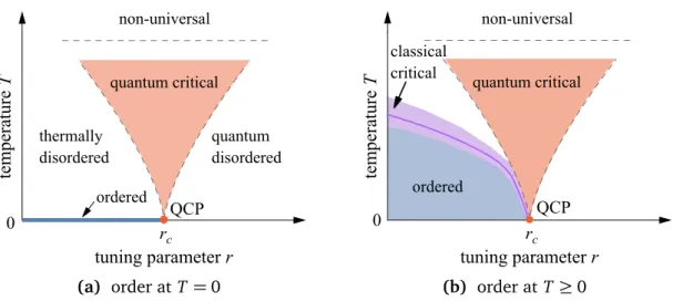
(a) order at T = 0 (b) order at T ≥ 0
Figure 2.1: Schematic finite-temperature phase diagrams close to a quantum critical point (QCP) at r = r
c. Dashed lines indicate crossovers. (a) Long-range order only at zero temperature. (b) An ordered phase extends to finite temperature, with the solid line marking the phase transition. In panel (b) the thermally disordered and quantum disordered regimes are still present, although not labeled. Figure based on Ref. [ 12 ] .
phase diagrams in the vicinity of a quantum critical point. We can distinguish two cases, depending on whether finite-temperature long-range order can exist.
In two-dimensional systems with an order parameter of continuous symmetry the Mermin-Wagner theorem [ 17 ] forbids long-range order at finite temperature.
Such a situation can lead to the phase diagram in Fig. 2.1a, where order only ex-
ists at T = 0 and no finite-temperature phase transitions occur. Nevertheless, the
finite-temperature behavior is characterized by three distinct regimes, separated by
crossovers. The quantum disordered region is dominated by quantum fluctuations
with the system resembling the quantum disordered ground state for r > r
c. The
elementary excitations on top of this ground state are typically well defined quasi-
particles with a finite energy gap ∆, such that their density at low temperatures
is exceptionally small. We have a thermally disordered region, where primarily
thermal fluctuations destroy the zero temperature order and the density of ther-
mally excited quasiparticles is again small. In an intermediate quantum critical
regime both quantum and thermal fluctuations are important. It is located above
the quantum critical point at r = r
cand its boundaries are determined by crossover
lines k
BT ∼ ~ω
c∼ | r − r
c|
νz. Here the picture of dilute quasiparticle excitations
does not apply. Physics in this region is controlled by thermal excitations of the
quantum critical ground state, typically characterized by the absence of conventional
quasiparticle excitations, which are replaced by a quantum critical continuum of
2.1 Introduction to quantum phase transitions
excitations. This leads to unusual features of the finite-temperature quantum critical region, including unconventional power laws and non-Fermi liquid behavior with uncommon transport properties. The behavior in this region is universal, but far away from the quantum critical point microscopic length scales begin to exceed the correlation length. Therefore quantum critical behavior is cut off at high temper- atures where k
BT is larger than characteristic microscopic energy scales such as a typical exchange energy. Here the physics is non-universal.
If order can also exist at finite temperatures, the richer phase diagram of Fig. 2.1b with a phase transition at low finite temperatures is established. Here the quantum critical point can be seen as the end point of a finite temperature transition line.
This line is surrounded by a classical critical regime, which becomes narrower as the quantum critical point is approached.
2.1.3 Scaling at quantum phase transitions
Thermodynamic properties can be derived from the partition function Z = Tr e
−H/kBTwith the Hamiltonian H = H
kin+ H
pot. In a classical system both parts of H commute and Z factorizes, Z = Z
kinZ
pot, such that statics and dynamics decouple. Usually singularities only occur in the static interacting part Z
pot. This allows us to study classical phase transitions with effective time-independent theories in d spatial dimensions.
For a quantum mechanical system, on the other hand, H
kinand H
potgenerally do not commute and Z does not factorize. Consequently, statics and dynamics are coupled and the order parameter field theory must be formulated in terms of space- and time-dependent fields. To do so, one introduces an imaginary time direction to the system, formally by applying the path integral representation of the partition function. At zero temperature the extent in this direction is infinite such that imaginary time acts as an additional spatial dimension, which by Eq. (2.2) scales with the zth power of a length. Therefore the homogeneity law (2.3) at T = 0 for a quantum phase transition reads
f ( t, B ) = b
−(d+z)f ( t b
1/ν, B b
yB) , (2.5) with t = ( r − r
c)/ r
c. In this way a quantum phase transition in d spatial dimensions is related to a classical transition in ( d + z ) dimensions. A generalization of Eq. (2.5) to finite temperature, where we recognize that we can approach the quantum critical singularity both by tuning r to r
cat T = 0 and by lowering T to zero at r = r
c, is
f ( t, B ) = b
−(d+z)f ( t b
1/ν, B b
yB, T b
z) . (2.6)
From the homogeneity law one can derive scaling relations for static and dynamic observables. For a correlation function C ( k, ω) at momentum k, measured relative to the ordering wavevector, and frequency ω we find for instance the following scaling relation at the quantum critical point:
C ( t = 0, k, ω , T = 0 ) = | k |
−dimCC
1(| k |
z/ω) , (2.7) where dim C is the scaling dimension of C . Similarly, at finite temperatures above the quantum critical point we obtain for k = 0:
C ( t = 0, k = 0, ω , T ) = T
−dimC/zC
2(ω/ T ) . (2.8) These naive scaling relations (2.7) and (2.8) are, however, only expected to be valid if the quantum critical point satisfies hyperscaling, which need not be true above the upper-critical dimension.
The value of the quantum-classical analogy can be seen by considering a correlation function G directly at a critical point. In a classical system of d dimensions critical correlations fall off with a power law in momentum space G ( k ) ∼ | k |
−2+ηd. For a quantum phase transition with dynamical critical exponent z = 1 we can conclude from the mapping at T = 0 that G (k, i ω
n) ∼ [k
2+ ω
2n]
(−2+ηd+1)/2where the Matsubara frequency ω
nacts as an extra component to k.
1By analytic continuation this translates to the retarded Green’s function at real frequencies G
R(k, ω) ∼ [k
2− (ω + i0
+)
2]
(−2+ηd+1)/2. This illustrates the excitation spectrum at a quantum critical point:
G
Rdoes not have a quasiparticle pole, but a branch cut at ω > | k | , corresponding to a continuum of excitations [4, Sec. 7.2].
2.1.4 Effective theories
Since the important physics at criticality is described by long-wavelength order parameter fluctuations, it can be appropriate to work with an effective theory of only these order parameter fluctuations that disregards microscopic details. Such a theory can formally be obtained by integrating out suitably decoupled interaction terms from a microscopic model. Since the correlation length is sufficiently large near a continuous transition, the effective action can be formulated in the continuum limit and will typically consist of powers of the order parameter field and of gradient terms. Its form will only depend on the symmetry and dimension of the underlying system and on the symmetry of the order parameter, consistent with the expectations
1
Here we assume the theory to be Lorentz invariant. Generally, additional terms of the form
f (ω/| k |) would be allowed.
2.1 Introduction to quantum phase transitions
for universal critical behavior. As an example consider a quantum rotor model H
rot= J g
2 X
i
~ L
2i− J X
〈i,j〉
~
n
i· n ~
j, (2.9)
with N-component operators ~ n
i, n ~
2i= 1 on the sites i of a d-dimensional lattice rep- resenting orientations and with the corresponding angular momenta ~ L
i. Minimizing the energy of the nearest-neighbor term favors an ordered ferromagnetic state, while the kinetic term prefers quantum-disordered delocalization. The parameter g tunes through a quantum phase transition.
A suitable order parameter for that transition is the ferromagnetic magnetization.
From the lattice model (2.9) a continuum theory is obtained in a spatial coarse graining procedure where the n ~
iare averaged over microscopic length scales. This yields the order parameter field ϕ, which is no longer of fixed length. An expansion to ~ lowest order in gradients of ϕ ~ produces a ϕ ~
4quantum field theory Z = R
D ϕ ~ exp(− S ) with action
S = Z
d
dx
Z
~/kBT 0d τ
1
2c
2(∂
τϕ) ~
2+ 1
2 (∇
xϕ) ~
2+ r
2 ϕ ~
2+ u
4 ϕ ~
22
. (2.10) Here r tunes the system across the quantum phase transition, c is a velocity, and u contains self-interactions of the fluctuations of ϕ ~ . The dynamical critical exponent is z = 1.
Eq. (2.10) provides a theory for quantum criticality that is appropriate for more models than just Eq. (2.9), with some non-conserved density as the order parameter field ϕ( ~ x, τ) . The approach of effective field theories of this kind has been very successful in treating quantum phase transitions in bosonic and insulating systems.
Suitable models can be solved exactly or are, more often, understood very well
in the framework of renormalization group theory with controlled expansions [ 4 ] .
Moreover, efficient unbiased numerical methods such as sign-problem-free quantum
Monte Carlo simulations are often available. These results confirm the general
phenomenology that we have outlined qualitatively in this Section. However, models
of itinerant electrons, adequate for the description of strongly correlated metals, can
frequently not be treated safely in effective theories of only local order parameter
fluctuations. Rather, low-lying fermionic excitations must be included explicitly in a
critical theory.
2.2 Quantum phase transitions in systems of itinerant electrons
Various quantum phase transitions in metals can be studied via effective models of itinerant electrons coupled to an order parameter field. Since in a metal there is an interplay between low energy fermionic quasiparticles at the top of the Fermi sea and the quantum fluctuations of this order parameter, the fermions cannot in general be safely integrated out without introducing divergences. Consequently such problems are intrinsically more complicated than quantum critical points in gapped insulators, which are captured by purely bosonic effective theories such as Eq. (2.10) that can be largely understood by mapping them to a classical theory.
The focus of this thesis is the quantum phase transition to antiferromagnetic order in a two-dimensional metal. To investigate the universal physics near such a quantum critical point we introduce in this Chapter a carefully motivated generic model of itinerant fermions coupled to a Néel spin-density wave order parameter at wavevector Q = (π , π)
ü. Magnetic quantum phase transitions in Fermi liquids are of considerable interest due to the rich physics that emerges from the quantum critical regime [5].
Beyond the scope of this work lie various other interesting quantum phase transitions in Fermi liquids, including the (Mott) metal-insulator transition [18], charge-density wave quantum critical points [19], or Ising-nematic quantum criti- cality [ 20, 21 ] .
2.2.1 Motivation of the spin-fermion model
In the momentum representation a microscopic Hamiltonian for a single band of itinerant S = 1/2 fermions subject to two-body interactions is given by
H
gen= H
kin+ H
int= X
k,s
"
kc
k,s†c
k,s+ X
ki,si
U
ks1,s2,s3,s41,k2,k3,k4
c
†k1,s1
c
k†2,s2
c
k3,s3
c
k4,s4
. (2.11) Here c
k,s†creates and c
k,sannihilates a fermion with momentum k and spin s =↑ , ↓ . On its own H
kinwould describe a tight-binding model with band-structure dispersion
"
k. In the additional H
intwe allow for a generic four-fermion interaction U
ks1,s2,s3,s41,k2,k3,k4
. For a generalized one-band Hubbard model [22] with local repulsion U > 0 the interaction term would be given by [ 23, Chapt. 3 ]
U
ks1,s2,s3,s41,k2,k3,k4
= U δ
0,k1+k2−k3−k4δ
s1,s3δ
s2,s4δ
s1,↑δ
s2,↓. (2.12)
2.2 Quantum phase transitions in systems of itinerant electrons
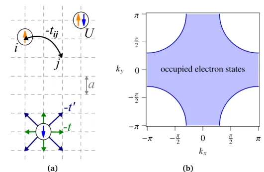
(a)
− π
−
π20
π2
π
k
y− π −
π20
π2π k
xoccupied electron states
(b)
Figure 2.2: (a) Illustration of the Hubbard model on a two-dimensional square lattice and visualiza- tion of nearest neighbor hopping t and next-nearest neighbor hopping t
0. (b) Sketch of the first Brillouin zone with a Fermi surface typical for a cuprate-like dispersion.
In real space with c
i,s†= p
1Ns
P
k
e
−ik·ric
k,s†the Hubbard Hamiltonian reads H
Hub= − X
i j,s
( t
i j+ µδ
i j) c
i,s†c
j,s+ U X
i
n
i,↑n
i,↓, (2.13)
where i, j ∈ { 1, . . . , N
s} label lattice sites, t
i jare hopping constants, µ is the chemical potential, and n
i,s= c
i,s†c
i,sare occupation number operators for spin s =↑, ↓ at site i.
In the following we will consider models of this type mainly on two-dimensional square lattices with unit lattice spacing a as sketched in Fig. 2.2a. Often we are interested in dispersion relations that yield Fermi surfaces akin to the sketch in Fig. 2.2b. These are appropriate for the electronic band structure of the cuprate superconductors, which can be well fitted by [ 24 ]
"
k= −2t (cos( k
x) + cos( k
y)) − 2t
0(cos( k
x+ k
y) + cos( k
x− k
y)) − µ, (2.14) where t > 0 is the hopping element for nearest neighbor sites and t
0< 0 the hopping element for next-nearest neighbor site. The other t
i jare zero.
To study the effects of magnetic order it is beneficial to rewrite the Hubbard
Hamiltonian in terms of local spin operators S ~
i= 1
2 X
ss0
c
†is(~ s )
ss0c
is0, ~ s = 0 1 1 0
,
0 − i i 0
,
1 0 0 − 1
ü, (2.15)
where ~ s are the Pauli matrices. Explicitly we have S ~
i= ( S
ix, S
iy, S
zi)
üwith S
ix= 1
2
c
i↑†c
i↓+ c
i↓†c
i↑
, (2.16a)
S
iy= − i 2
c
i↑†c
i↓− c
†i↓c
i↑
, (2.16b)
S
iz= 1 2
n
i↑− n
i↓
. (2.16c)
As in, for example, [ 23, Chapt. 2 ] we find H
Hub= X
k,s
"
kc
†k,sc
k,s− 2U 3
X
i
S ~
i2+ U 2
X
i,s
n
i,s= X
k,s
" ˜
kc
†k,sc
k,s− U 6N
sX
a,b,c,d
=↑,↓
X
k1,k2, q
c
k†1+q,a
(~ s )
a bc
k1,b
· c
k†2−q,c
(~ s )
cdc
k2,d
. (2.17) Since the term in n
i,sonly renormalizes the chemical potential, we let ˜ "
kabsorb it in the second line and will drop the tilde in the following. From this transformed form of the Hubbard Hamiltonian we can now easily move to a slightly more general specification of the generic Hamiltonian in Eq. (2.17):
H = X
k,s
"
kc
k,s†c
k,s− 1 4N
sX
k1,k2,q, a,b,c,d
V ( q ) c
k†1+q,a
(~ s )
a bc
k1,b
· c
†k2−q,c
(~ s )
cdc
k2,d
, (2.18) where we now allow for an arbitrary interaction with momentum transfer q in the spin channel, V ( q ) = V (− q ) . We would recover H
Hubby setting V ( q ) =
2U3. The remaining quartic term in Eq. (2.18) needs to be treated with some care. First, we write the grand-canonical partition function of a system governed by H at temperature T = 1 /β as a functional field integral [ 25, Sect. 4.2 ]
Z = Tr e
−βH= Z
D ( c
†, c ) e
−S[c†,c](2.19)
2.2 Quantum phase transitions in systems of itinerant electrons
with the action S [ c
†, c ] = S
kin+ S
intand S
kin=
Z
β 0d τ X
k,s
c
k,s†(τ)[∂
τ+ "
k] c
k,s(τ) , (2.20a)
S
int= − 1 4
Z
β 0d τ X
k1,k2,q, a,b,c,d
V (q) c
k†1+q,a
(τ)[~ s ]
a bc
k1,b
(τ) · c
k†2−q,c
(τ)[~ s ]
cdc
k2,d
(τ).
(2.20b) We use the same symbols c
†, c interchangeably for Grassmann variables and fermionic operators in Fock space. With this change of language from Hamiltonian to action it is straightforward to decouple the interaction via a Hubbard-Stratonovich trans- formation, see [ 26, Chapt. 3 ] and [ 25, Sect. 6.2 ] . Formally, this amounts to the application of a standard identity for real Gaussian integrals
Z
dv e
−12vüAv+jüv= ( 2 π)
N/2det A
−1/2e
12jüA−1j, (2.21) where v is a real N -component vector, A is a real symmetric N × N matrix, and j is an arbitrary N -component vector.
To apply (2.21) we set % ~
q(τ) = P
k,a,b
c
k†+q,a(τ)[~ s ]
a bc
k,b(τ) and for each τ form a vector %(τ) ~ containing % ~
qfor each distinct momentum q. From the values V ( q ) we construct an antidiagonal symmetric matrix V, which allows us to write S
intin a shortened notation:
e
−Sint= exp
¨Z
β 0d τ 1 4
X
q
~
%
q(τ) V (q) % ~
−q(τ)
«
(2.22)
= exp
¨Z
β 0d τ 1
4 %(τ) ~
ü· V · %(τ) ~
«
. (2.23)
Now we can put Eq. (2.21) to use at each τ and find (dropping arguments τ ):
exp
§ 1
4 % ~
ü· V · % ~ ª
= const · Z
d ϕ ~ exp ¦
− ϕ ~
ü· V
−1· ϕ ~ + % ~
ü· ϕ ~ ©
= const · Z
d ϕ ~ exp ¦
− ϕ ~
ü· V · ϕ ~ + % ~
ü· V · ϕ ~ ©
. (2.24)
Here the integration variable ϕ ~ is a vector built from three real numbers ϕ ~
qfor each distinct momentum q. The constant factors in front of the integrals are irrelevant for expectation values computed from Z and for the functional integrals we will include them in the integration measure. In the second line of Eq. (2.24) we have transformed the integration variable ϕ ~ → V ϕ ~ . Both forms are equivalent.
In this way we have effectively traded the four-fermion interaction in for an auxiliary bosonic field ϕ ~ . The partition function is now given by the functional integral over fermionic and bosonic fields with a coupled action:
Z = Z
D ( c
†, c, ϕ) ~ e
−(Skin[c†,c]+SFB[c†,c,ϕ]+~ SB[ϕ])~, (2.25a) S
kin=
Z
β 0d τ X
k,s
c
k,s†[∂
τ+ "
k] c
k,s, (2.25b)
S
FB= Z
β0
d τ X
k,q,a,b
V (q) c
k†+q,a[~ s ]
a bc
k,b· ϕ ~
−q, (2.25c)
S
B= − Z
β0
d τ X
q
~
ϕ
qV (q) ϕ ~
−q. (2.25d)
Eq. (2.25) constitutes the spin-fermion model [6, 27, 28]. The spin-fermion model is to be thought of as having arisen from a microscopic Hamiltonian, from which high- energy degrees of freedom, i.e. behavior at energies comparable to the fermionic bandwidth W , have been integrated out. Thus it can serve as an effective theory at energies smaller than a cutoff Λ < W . We can understand the spin-fermion model as describing low-energy fermions which interact with their own spin fluctuations.
Due to the separation of energy scales these collective modes appear as autonomous bosonic spins ϕ ~
q. The spin-fermion model is often stated as a Hamiltonian of itinerant electrons c and spins ϕ ~
H
sf= X
k,s
0
v
F( k − k
F) c
k,s†c
k,s+ X
q
0
χ
0−1( q ) ϕ ~
qϕ ~
−q+ g X
k,q,a,b
0
c
k+q,a†[~ s ]
a bc
k,b· ϕ ~
−q,
(2.26)
where the primed sums limit momenta below Λ . Here the low-energy fermion
propagator retains Fermi-liquid form, but note that the electronic dispersion "
khas
been linearized for momenta k close to the Fermi surface at k
Fwith the Fermi velocity
v
F= ∂
k"
k|
kF. The bare boson susceptibility is taken as χ
0−1( q ) = χ
0/[ξ
−02+ ( q − Q )
2]
2.2 Quantum phase transitions in systems of itinerant electrons
with a bare magnetic correlation length ξ
0and the ordering wavevector Q. g is introduced as a coupling constant, which must be small compared to W . The value of Q has been determined by higher energy interactions and, like the other parameters, should be considered as input to the theory; for commensurate antiferromagnetic Néel order in two dimensions it is Q = (π, π)
ü.
The action (2.25) should be thought of as an effective theory on its own right for the underlying strongly correlated microscopic system. We will use a variation of this model to study a metal close to a spin-density wave quantum critical point where it will capture the universal physics. While we have sketched the derivation from a microscopic Hamiltonian, this Hamiltonian may actually not be known for certain and the resulting action (2.25) stands independent of its formal derivation.
2.2.2 Metal close to the onset of spin-density wave order
Having outlined how the spin-fermion model (2.25) can be obtained from a Hubbard- like Hamiltonian, we now specify the formulation we shall use to study a two-dimen- sional metal close to a spin density wave (SDW) quantum critical point (QCP).
Our choice follows [ 4, Chapt. 18 ] . In a slight extension to the derivation in the last Section we allow the bare bosonic susceptibility to depend on frequency. We define the real bosonic field ϕ ~
qto represent long-wavelength fluctuations with small momentum q around collinear SDW order at wavevector Q = (π , π)
ü, such that ϕ ~
qcorresponds to the electron spin density at Q + q.
2The bosonic action is given by a Ginzburg-Landau ϕ
4theory similar to Eq. (2.10), which can be thought to have been generated by integrating out high-energy electrons. The complete model has the action S = S
F+ S
F B+ S
Bwith
S
F= Z
β0
d τ X
k,s
c
k,s†[∂
τ+ "
k] c
k,s, (2.27a)
S
FB= λ Z
β0
d τ X
k,q,s,s0
c
k†+Q+q,s[~ s · ϕ ~
q]
ss0c
k,s0= λ Z
β0
d τ X
i,s,s0
e
iQ·ric
†i,s[~ s · ϕ ~
i]
ss0c
i,s0, (2.27b) S
B=
Z
β 0d τ X
i
1
2c
2(∂
τϕ ~
i)
2+ 1
2 (∇ ϕ ~
i)
2+ r
2 ϕ ~
2i+ u
4 ϕ ~
2i2
. (2.27c)
2
Compared to the action (2.25) this is a shift ϕ ~
q→ ϕ ~
Q+q.
Here, λ is the “Yukawa coupling” constant between fermionic and bosonic fields, c is the bare bosonic velocity, and the parameters r and u control the magnitude of the SDW fluctuations. In a mean-field theory for S
Balone long-range SDW order is present for r ≤ 0, but this transition point is shifted by interactions. The derivatives in Eq. (2.27) need to be discretized appropriately for the actual space-time lattice.
A first understanding of the physics of the combined model (2.27) can be found in mean-field theory. We can distinguish two phases: a Fermi liquid with 〈 ϕ〉 ~ = 0 and an ordered SDW phase with 〈 ϕ〉 6= ~ 0. To describe them on mean-field level we replace in S
FBthe field ϕ ~
qby its uniform expectation value 〈 ϕ ~
q〉
MF= δ
q,0ϕ ~
0, corresponding to perfect Néel order, and drop the action S
Bfor the now constant field. This procedure can be motivated by a saddle point approximation of S. Since rotational symmetry is broken spontaneously in the ordered phase, different directions of ϕ ~
0are equivalent and only its magnitude is important. Returning from the functional integral formalism, we obtain the mean-field Hamiltonian
H
MF= X
k,s
"
kc
k,s†c
k,s+ λ X
k,s,s0
c
k†+Q,s[~ s · ϕ ~
0]
ss0c
k,s0. (2.28) In mean field the SDW order ϕ ~
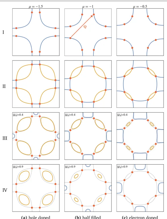
0mixes only fermionic states at momenta k and k + Q. Consequently, there is only a restricted set of zero-energy states (measured relatively to the chemical potential) on the Fermi surface that interact in H
M F. They are found by taking the intersection of the Fermi surface and the Fermi surface shifted by Q. If there is no intersection, e.g. if the Fermi surface for a cuprate-like dispersion (2.14) is too small, there is no SDW interaction at low energies. Otherwise in two dimensions we typically find a discrete set of intersection points. These are the “hot spots” illustrated in rows I and II of Fig. 2.4. As far as the low-energy physics of the action (2.27) is concerned, the close vicinities of the hot spots will remain the most important regions of the Brillouin zone also beyond mean field. There an electron at k may scatter into a state at k + Q + q, but q will generally be small compared to the size of the Brillouin zone for the predominating ϕ ~
q.
With the help of spinors d
k†=
c
k,†↑, c
†k,↓, c
k†+Q,↑, c
k†+Q,↓
we can write the Hamiltonian in the form H
MF= P
0k
d
k†h
kd
k, where the primed sum indicates that the summation now runs over a smaller set of momenta k and h
kis a 4 × 4-matrix
h
k=
"
k"
kλ ~ ϕ
0· ~ s λ ~ ϕ
0· ~ s "
k+Q"
k+Q
. (2.29)
2.2 Quantum phase transitions in systems of itinerant electrons
(a) "
k(b) e
k,±Figure 2.3: 3D plots of (a) the original dispersion "
kfrom Eq. (2.14) with t = 1, t
0= − 0.5, µ = − 0.5, and of (b) the hybridized mean-field dispersion e
k,±from Eq. (2.30) for SDW order | ϕ ~
0| = 0.4.
The Fermi surfaces are marked by gray lines, compare Fig. 2.4c.
This matrix is easily diagonalized and we find two-fold degenerate single-electron energy eigenvalues
e
k,±= "
k+ "
k+Q2 ±
v u t
"
k− "
k+Q2
2+ (λ ~ ϕ
0)
2. (2.30) In the presence of SDW order, e
k,±give the dispersion for two electronic bands. Filling up the lowest-energy states both bands we find the new Fermi surface as illustrated in Fig. 2.3. For | ϕ ~
0| > 0 gaps open at the hot spots and the originally “large” Fermi surface is reconstructed into “small” Fermi pockets, see row III in Fig. 2.4. As | ϕ ~
0| increases, these pockets shrink. For the half-filled system they vanish simultaneously, in the hole-doped case the electron pockets disappear first, while in the electron- doped case the hole pockets disappear first, see row IV in Fig. 2.4. A configuration of small Fermi pockets is a generic feature of an SDW-ordered Fermi liquid.
2.2.3 Analytical approaches beyond mean field
The pioneering work on quantum criticality in Fermi liquids was presented by Hertz
[ 29 ] , who studied magnetic transitions by a renormalization group method. Millis
later extended this work and added the evaluation of finite-temperature crossovers
[30]. In Hertz-Millis theory the fermions are integrated out and only low-energy
order parameter fluctuations are kept in the action. While this step is formally exact,
in the presence of gapless fermionic excitations the resulting coefficients can be
highly non local. A priori it is not clear that such an action can be expanded in ϕ ~
I
μ -
Q
μ -
II
III
|φ0|=0.4 |φ0|=0.4 |φ0|=0.4
IV
|φ0|=0.9 |φ0|=0.9 |φ0|=0.9
(a) hole doped (b) half filled (c) electron doped
Figure 2.4: Mean-field transformation of the Fermi surface due to SDW order for Eq. (2.14) with
t = 1, t
0= − 0.5, and (a) µ = − 1.5, (b) µ = − 1, (c) µ = − 0.5. The momentum k = ( 0, 0 )
üis at
the center of each plot, as in Fig. 2.2b. Row I: Fermi surface without SDW order with hot spots
separated by Q = (π , π)
ü. Row II: Original Fermi surface together with surface shifted by Q; hot
spots are at the intersection points. Row III: Small Fermi surfaces with SDW order | ϕ ~
0| = 0.4,
computed from Eq. (2.30). Row IV: With | ϕ ~ | = 0.9 electron pockets have shrunk to zero in case
2.2 Quantum phase transitions in systems of itinerant electrons
Figure 2.5: Proposed schematic phase diagram in the vicinity of an antiferromagnetic metallic quan- tum critical point. Next to a spin-density wave (SDW) ordered phase a d-wave superconducting (SC) dome emerges atop the quantum critical point (QCP). Compare to Fig. 2.1.
and that a controlled truncation of this expansion is possible. Assuming that one can proceed in this way, the resulting action for the case of the ordering wave vector Q connecting a ( d − 2 ) -dimensional hot manifold is
S =
Z d
dk (2π)
dT X
ωn