Synthetic [C ii ] line emission maps of simulated interstellar medium

Synthetic [C ii ] line emission maps of simulated interstellar medium

I naugural – D issertation

zur

Erlangung des Doktorgrades

der Mathematisch – Naturwissenschaftlichen Fakult¨at der Universit¨at zu K¨oln

vorgelegt von

Annika Franeck

aus Berlin-Pankow

K¨oln, 2018

Berichterstatter: Prof. Dr. Stefanie Walch-Gassner Prof. Dr. J¨urgen Stutzki

Tag der m¨undlichen Pr¨ufung: 10. September 2018

“Hilf mir aus dem Rachen des L¨owen, und errette mich von den Einh¨ornern.”

Psalm 22,22

Abstract

In this thesis I analyse the synthetic [C ii ] emission from a slice of interstellar medium (ISM). The [

C ii ] line emission is the fine structure transition in carbon ions. It is observed in several phases of the ISM, such as the molecular, warm, and ionized gas phases. By analysing the [

C ii ] line emission in observations, one would like to estimate the star formation rate, and the fraction of molecular hydro- gen in the studied objects. However, for those studies it is crucial to disentangle from which gas phase the [C ii ] line emission stems. We therefore study the [C ii ] line emission in 3D numerical simulations.

The underlying simulations represent (i) a piece of a galactic disc (SILCC-Project

Walch et al., 2015, Girichidis et al., 2016b), in which the ISM is stirred by the explosions of SNe; the positioning of the SNe determines the gas phases formed in the ISM. In a second setup, (ii) a forming molecular cloud before the onset of star formation (MC2) is simulated (SILCC-Zoom project Seifried et al., 2017). We carry out radiative transfer simulations with radmc -3 d (Dullemond, 2012) for the [

C ii ] line emission. We expect the [

C ii ] line emission to be observable for I

≥ 0.5 K km s

, and find for MC2 that ∼20% of the total projected area is above this detection limit, contributing ∼80% to the total luminosity in [

C ii ].

Thus, we conclude that molecular clouds before the onset of star formation are ob- servable in [

C ii ]. We find the [

C ii ] emission to be optically thick, in the densest regions, ∼40% of the observable area for MC2. We estimate the emission line of the strongest hyperfine structure transition [

C ii ] (F = 2 − 1) from the carbon ion isotope

C

to use it as an optically thin analogue to [

C ii ].

We analyse the distribution of the [

C ii ] line emission in the SILCC setups, and find the vertical emission profiles to have in general a complex structure. In almost all simulations there is a dominant peak of the [

C ii ] line emission from the molec- ular clouds located in the midplane. To characterize the distribution of the emission, we calculate its variance, and define the square root of the variance as a scale height.

For most of the simulations the scale height is . 100 pc. We find the scale height to trace the outflowing component of the gas.

We study the origin of the [C ii ] line emission with the optically thin tracer [

C ii ].

For the SILCC simulations we find the [C ii ] line emission correlated with the molecular gas phase. For the zoom-in simulation MC2, having a better spatial res- olution, and no further feedback processes included, we find the [C ii ] line emis- sion to stem from the atomic gas with physical properties as 43 K ≤ T ≤ 64 K, 53 cm

≤ n ≤ 438 cm

, with a range of 16% to 44% of the hydrogen in molec- ular form, and a visual extinction A

between 0.5 ≤ A

≤ 0.91. We test further

1

SILCC: Simulating the Life Cycle of molecular Clouds, project led by S. Walch

7

whether the result changes by the resolution of the simulation, and find the tem- perature range to be una ff ected, whereas the number density and the fraction of molecular hydrogen change slightly. However, the overall conclusion holds for all zoom-in simulations.

We study the correlation between the integrated [

C ii ] intensity with the column densities of the total gas, H, and C

, and find the distributions to follow power- laws with slopes of ∼0.7, 0.5, and 0.6, respectively. We define a Y

factor, which is the ratio between the column density of the total gas, and the integrated [

C ii ] intensity. Estimated over the whole emission map, we find the median value as Y

≈ 1.1 × 10

cm

(K km s

)

. In general it scales with Y

∝ I

.

We analyse the line profiles by comparing them with two reference functions, a Gaussian and a Boxcar function, representing an optically thin and thick line. We define a Tauber value as the di ff erence between the reference function and the line profile, normalized by the amplitude of the reference function. We find no specific tendencies for the Tauber values in the [

C ii ] line. However, the values we obtain are comparable to Tauber values derived from observed data.

Finally, we carry out synthetic emission maps of the

CO (1–0),

CO (1–0), and

C

O (1–0) line emissions, and the H i 21 cm line. We calculate the H i line with

di ff erent approaches for the spin temperature, and find the spin temperature to be

equal to the kinetic gas temperature for most parts in the simulation. We compare

the integrated [

C ii ] and H i line emission, and find no correlation of these quan-

tities in the observable range of [

C ii ]. In a comparison of the synthetic [

C ii ]

and

CO (1–0) emission maps, we find a fraction of 80% of the total H

mass to

be aligned with the observable

CO (1–0) line emission, and 90% with the observ-

able [

C ii ] line emission. Thus, about 10% of the H

mass is CO-dark H

, and the

remaining 10% of H

mass is not detected in the [

C ii ] or the

CO (1–0) line.

Zusammenfassung

In der vorliegenden Arbeit geht es um synthetische Emissionskarten der [C ii ] Linie von Simulationen des interstellaren Mediums (ISM). Die [

C ii ] Linie ist die Linie des Feinstruktur¨ubergangs im Kohlensto ffi on, und wird im Universum sowohl in der kalten, molekularen Gasphase, als auch in der warmen, ionisierten Phase beobachtet.

Um mithilfe der [

C ii ] aus Beobachtungen auf die Sternentstehungsrate, oder den Anteil von H

schliessen zu k¨onnen, ist es wichtig zu verstehen, aus welcher Gas- phase die beobachtete [

C ii ] Emission stammt. Dies untersuchen wir in dieser Arbeit anhand von numerischen Simulationen.

Als Simulation verwenden wir dabei die (i) SILCC

Simulationen (Walch et al., 2015, Girichidis et al., 2016b), die das ISM in einem Teil einer Galaxiescheibe repr¨asentieren, und (ii) in einer zoom-in Simulation MC2 (SILCC-Zoom Projekt, Seifried et al., 2017), in der die Formation einer Molek¨ulwolke untersucht wird.

Wir berechnen von den fertigen Simulationen die Emissionskarten der [

C ii ] Linie mit radmc -3 d (Dullemond, 2012). Wir erwarten, dass man die [

C ii ] Linie ab einer Intensi¨at von 0.5 K km s

detektieren kann, und finden, dass ∼20% der pro- jizierten Gesamtfl¨ache in MC2 beobachtbar sind. Diese beobachtbare Fl¨ache tr¨agt mit 80% zur Gesamtluminosit¨at der [

C ii ] Emission bei. Die [

C ii ] Linie ist optisch dick ¨uber ∼40% der beobachtbaren Fl¨ache. Wir berechnen zus¨atzlich die [

C ii ] (F = 2 − 1) Linie, welche die st¨arkste Linie der Hyperfein¨uberg¨ange im Kohlensto ffi onenisotop

C

ist, um ein optisch d¨unnes ¨ Aquivalent zur [

C ii ] Linie zu erhalten.

In den SILCC Simulationen untersuchen wir die vertikale Verteilung der [

C ii ] Strahlung um die galaktische Scheibe. In unseren Simulationen zeigt das Profil eine sehr komplexe Struktur. Das vertikale Emissionsprofil wird durch die starke Strahlung von den Molek¨ulwolken aus der Galaxiescheibe dominiert. Wir quan- tifizieren die vertikale Verteilung der Emission, indem wir ihre Varianz berechnen.

Die Wurzel aus der Varianz definieren wir als Skalenh¨ohe. Die Skalenh¨ohen sind in der Gr¨ossenordnung von . 100 pc f¨ur die meisten Simulationen, und bilden ein Maß f¨ur das ausstr¨omende Gas aus der Galaxiescheibe.

Ein Hauptanliegen dieser Arbeit besteht in der Charakterisierung des Gases, welches die [C ii ] Linie emittiert. Dies untersuchen wir mit der optisch d¨unnen [

C ii ] Linie.

In den SILCC Simulationen finden wir einen Zusammenhang zwischen der [C ii ] Emission und der molekularen Gasphase. In der besser aufgel¨osten Simulation MC2 kommt die [C ii ] Linie aus Gas mit Temperaturen zwischen 43 K ≤ T ≤ 64 K, mit Teilchenzahldichten zwischen 53 cm

≤ n ≤ 438 cm

, in denen zwischen 16% und 44% des Wassersto ff s als H

vorliegt, und das eine visuelle Extinktion

2

SILCC: Simulating the Life Cycle of molecular Clouds, gef¨uhrt von S. Walch

9

zwischen 0.5 ≤ A

≤ 0.91 hat. Folglich stammt die [C ii ] Emission aus der atom- aren Gasphase, in dem sich H im ¨ Ubergang zu H

befindet. Diese Schlussfolgerung finden wir bei anderen Aufl¨osungen und anderen Simulationen best¨atigt.

Wir untersuchen weiterhin den Zusammenhang zwischen der integrierten [

C ii ] Intensit¨at und der S¨aulendichte des gesamten Gases, H und C

. In allen drei F¨allen l¨asst sich dieser mit einem Potenzgesetz beschreiben. Wir definieren weiterhin einen Y

Faktor als Verh¨altnis zwischen der S¨aulendichte und der [

C ii ] Inten- sit¨at. Der Y

Faktor skaliert im allgemeinen mit der [

C ii ] Intensit¨at als Y

∝ I

.

Schließlich berechnen wir Emissionskarten bei den Wellenl¨angen der H i 21 cm

Linie und den

CO (1–0),

CO (1–0), C

O (1–0) Linien. Die H i Linie berechnen

wir mit verschiedenen Annahmen f¨ur ihre Spintemperatur; das Ergebnis zeigt dass

die Spintemperatur in großen Teilen der Simulation identisch mit der kinetischen

Temperatur des Gases ist. Wir finden keine Korrelation der integrierten H i und

[

C ii ] Intensit¨at im beobachtbaren Bereich von [

C ii ]. Dies kann mit der optis-

chen Tiefe der Linien zusammenh¨angen, als auch ein Hinweis darauf sein, dass die

H i Linie aus einem gr¨osseren Bereich als das [C ii ] emittierende Gas stammt. Weit-

erhin untersuchen wir welcher Massenanteil von H

entlang von Sichtlinien von

[

C ii ] und

CO (1–0) existiert. Im Bereich des beobachtbaren

CO (1–0) liegen

80% der H

Masse, und im beobachtbaren [

C ii ] Bereich 90% der H

Masse. Fol-

glich sind 10% der H

Masse CO dunkles Gas, und weitere 10% weder in [

C ii ]

noch in

CO (1–0) detektierbar.

Contents

Abstract 9

Zusammenfassung 11

List of Figures 22

List of Tables 24

1 Introduction 27

1.1 The Milky Way . . . . 27

1.2 The interstellar medium . . . . 29

1.2.1 Processes in the ISM . . . . 30

1.2.2 Phases of the ISM . . . . 34

1.2.3 Molecular clouds . . . . 35

1.3 Radiation detected from the ISM . . . . 39

1.3.1 Carbon monoxide, CO . . . . 40

1.3.2 Ionized carbon, [C ii ] . . . . 41

1.3.3 Atomic hydrogen, H i . . . . 41

1.4 [C ii ] Surveys . . . . 42

1.5 Simulations . . . . 46

1.5.1 Numerical simulations of the ISM . . . . 46

1.5.2 Radiative transfer simulations . . . . 48

1.6 Purpose of this thesis . . . . 49

2 Simulations 53 2.1 General remarks about the SILCC simulations . . . . 53

2.2 Simulation setups . . . . 56

2.2.1 SILCC-01: SILCC with fixed SNe . . . . 56

2.2.2 SILCC-02: Simulations with sink particles . . . . 62

2.2.3 Zoom in simulations . . . . 63

3 Radiative transfer simulations 69 3.1 Basic concepts on radiative transfer . . . . 69

3.2 Transition in carbon ions . . . . 71

3.2.1 Fine structure transition of

C

. . . . 71

3.2.2 Hyperfine structure transition of

C

. . . . 72

3.3 Radiative transfer with radmc -3 d . . . . 74

3.3.1 Implementation and assumption in radmc -3 d . . . . 74

13

3.3.2 Input parameters for radmc -3 d . . . . 76

3.3.3 Output of RADMC-3D . . . . 80

3.4 Synthetic [C ii ] emission maps . . . . 82

4 Testing the simulations 87 4.1 Test with the SILCC setup . . . . 88

4.1.1 Modes for the calculations in radmc -3 d . . . . 88

4.1.2 Variation of the microturbulence . . . . 91

4.1.3 Optical depth within the SILCC setup . . . . 92

4.2 Tests with the zoom-in simulation MC2 . . . . 95

4.2.1 Optical depth within MC2 . . . . 95

4.2.2 Spatial convergence of the synthetic emission maps . . . . . 98

4.2.3 Spectral convergence of the synthetic emission maps . . . . 101

4.2.4 Testing a microturbulence according to Larson . . . 103

4.2.5 Testing escape probability lengths L

. . . 104

4.3 Setup of a molecular cloud . . . 105

4.3.1 Molecular cloud inspired from the SILCC simulations . . . 105

4.3.2 Molecular cloud at higher densities . . . 109

4.4 Discussion . . . 111

5 Distribution of the [C ii ] emission 113 5.1 Theory . . . 113

5.1.1 Scale height via Gaussian fitting . . . 113

5.1.2 Scale height via Variance . . . 114

5.2 Analysis . . . 115

5.2.1 Analysis of S10-KS-rand . . . 115

5.2.2 Analysis of SILCC with fixed SNe . . . 119

5.2.3 Analysis of SILCC with sink particles . . . 121

5.3 Convolution with a Gaussian beam . . . 122

5.4 Discussion . . . 125

5.4.1 Comparison with observations . . . 125

5.4.2 Influences on the simulations . . . 127

6 Origin of the [C ii ] line emission 131 6.1 Simulations with a fixed SNR . . . 132

6.1.1 Temperature dependence . . . 132

6.1.2 Density dependence . . . 135

6.1.3 Molecular hydrogen dependence . . . 138

6.1.4 Visual extinction dependence . . . 139

6.2 Simulations with sink particles . . . 139

6.2.1 Temperature dependence . . . 139

6.2.2 Density dependence . . . 141

6.2.3 Molecular hydrogen dependence . . . 144

6.2.4 Visual extinction dependence . . . 145

6.3 Zoom-in simulations . . . 146

6.3.1 Temperature dependence . . . 146

6.3.2 Density dependence . . . 149

6.3.3 Molecular gas dependence . . . 149

15

6.3.4 Visual extinction dependence . . . 151

6.3.5 Origin of the emission, analysed with an optically thick tracer151 6.3.6 Origin of the emission at di ff erent spatial resolution . . . 153

6.3.7 Testing di ff erent clouds and di ff erent times . . . 157

6.4 Comparison . . . 157

6.5 Discussion . . . 159

6.5.1 Comparison with observations . . . 159

6.5.2 Comparison with other simulations . . . 161

7 Correlation of the [C ii ] line emission with the number density 163 7.1 Direct correlation . . . 163

7.2 Correlation analysed with Y

. . . 165

8 Line profiles 169 8.1 Examples of line profiles . . . 171

8.2 Tauber method . . . 174

8.3 Line profiles at di ff erent resolution levels . . . 181

8.4 Line profiles for the zoom-in molecular cloud MC1 . . . 185

8.5 Discussion . . . 187

9 Complementary synthetic emission maps 189 9.1 H i emission line . . . 190

9.1.1 Hyperfine structure transition atomic carbon . . . 190

9.1.2 Level population in H i . . . 190

9.1.3 Synthetic H i emission maps for the SILCC setup . . . 194

9.1.4 Synthetic H i emission maps for MC2 . . . 196

9.2 CO emission lines . . . 200

9.2.1 Rotational CO emission lines . . . 200

9.2.2 Synthetic CO emission maps for MC2 . . . 201

9.3 Line profiles . . . 205

9.4 Discussion . . . 205

10 Conclusion and Outlook 209 10.1 Conclusion . . . 209

10.2 Outlook . . . 214

Acknowledgements 217

List of Abbreviations and constants 229

List of Figures

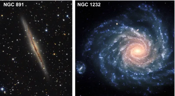
1.1 Sketch of the composition of the Milky Way, taken from Buser (2000), fig. 1 therein. . . . 28 1.2 The Milky Way, as seen with the Planck satellite. . . . 28 1.3 Milky Way like galaxies NGC 891 and NGC 1232 . . . . 30 1.4 Cooling curve for the neutral atomic gas from Dalgarno & McCray

(1972) and Gnat & Ferland (2012) . . . . 33 1.5 Schematic representation of the equilibrium curve, illustrating the

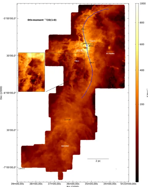
resulting two phases of the ISM (credit: Tielens et al. 2005) . . . . 34 1.6 Orion molecular cloud as presented in Kong et al. (2018), fig. 5

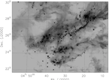
therein. . . . 37 1.7 Taurus molecular cloud complex, as presented in Goldsmith et al.

(2008), fig. 14 therein. . . . 38 1.8 Transmission of the radiation through the atmosphere of the Earth . 39 2.1 Column density maps of the total gas in the SILCC-01 and SILCC-

02 simulations. . . . . 59 2.2 Phaseplots of some of the SILCC simulations. . . . 60 2.3 Synthetic [

C ii ] line emission maps and column densities for MC2. 64 2.4 Mass-weighted two-dimensional histogram of the zoom-in simu-

lation MC2, for the total gas, and the relevant chemical species. . . 65 3.1 Energy scheme of the C

ion. . . . 73 3.2 Mass distribution of C

ions in the simulation S10–KS–rand at

t = 50 Myr before and after correcting the number densities. . . . . 78 3.3 De-excitation rates for the collisions of C

with ortho- and para-

H

, H, and electrons . . . . 79 3.4 Aceraged [

C ii ] spectrum of the simulations S10–KS–rand, and

MC2 at di ff erent wavelengths . . . . 80 3.5 [

C ii ] synthetic emission maps of the SILCC simulations (SILCC-

01 and SILCC-02). . . . 83 3.6 Synthetic [

C ii ] emission maps of the zoom-in simulation MC2

for di ff erent projections. . . . 85 3.7 Synthetic [

C ii ] emission maps of the zoom-in simulation MC2

for di ff erent projections, showing the integrated intensity on linear scale. . . . 85

17

18 L ist of F igures 4.1 Synthetic [

C ii ] line emission maps for S10-KS-rand at t = 50 Myr,

testing the radmc -3 d modes, and the influence on the result con- cerning the origin of the maps. . . . 89 4.2 Intensity profiles of the synthetic [

C ii ] line emission maps for the

simulation S10–KS–rand at t = 50 Myr calculated with di ff erent modes in radmc -3 d . . . . 89 4.3 Vertical profiles of the [

C ii ] line emission maps for the simula-

tion S10–KS–rand at t = 50 Myr for di ff erent microturbulences. . . 91 4.4 Histogram of the amount of optically thin and thick pixels as a

function of the column density of the total gas N

for the SILCC simulation S10–KS–rand. . . . 93 4.5 Maps of the SILCC simulations, indicating where and over which

velocity range the [

C ii ] line emission becomes optically thick. . 94 4.6 Maps of MC2 in di ff erent projections, indicating where and over

which velocity range the [

C ii ] line emission becomes optically thick. . . . . 95 4.7 Histogram indicating at which total gas column density the [

C ii ]

line emission becomes optically thick . . . . 96 4.8 Two-dimensional histograms of T

and T

for the [

C ii ] and

[

C ii ] line emission. . . . . 97 4.9 Two-dimensional histograms of T

for the [

C ii ] and [

C ii ] line

emission. . . . . 97 4.10 Opacity a ff ected [

C ii ] line emission maps of the zoom-in simu-

lations in the xz-projection at di ff erent resolutions. . . . 99 4.11 Opacity a ff ected [

C ii ] line emission maps of the zoom-in simu-

lations in the xz-projection at di ff erent resolutions. . . . 99 4.12 Convergence study of the [

C ii ] emission maps, with respect to

their spatial resolution, analysed for the luminosity, and peak inte- grated intensity. . . . 100 4.13 As Fig. 4.12, this time for the [

C ii ] (optically thin [C ii ]) line

emission. All projections have identical luminosities, so that they fall on to one curve (left). . . 100 4.14 Histograms of the integrated intensities of the [

C ii ] (opacity af-

fected [C ii ]) and the [

C ii ] (optically thin [C ii ]) line emission.

. . . 102 4.15 Median deviation for the integrated [

C ii ] line emission maps at

di ff erent spectral resolutions, as indicated on the x-axis. . . 102 4.16 Histograms of the integrated intensities for the synthetic [

C ii ]

emission maps at di ff erent resolutions, assuming a microturbu- lence according to Larson (1981). . . . 103 4.17 Histograms of the integrated intensities for the synthetic [

C ii ]

line emission maps, calculated with the LVG approximation with di ff erent escape length probabilities L

(lines mode = 3), and for the optical thin approximation (lines mode = 4). . . 104 4.18 Two-dimensional histograms of the excitation temperatures T

for

the calculations with L

= ∞ versus L

= 70 pc (left) and

L

= ∞ versus L

= 0.5 pc (right). . . . 105

L ist of F igures 19 4.19 Number density along a line of sight towards the centre of the

molecular cloud, which is at z = 0 pc, for the total gas (upper left panel) and the di ff erent chemical species, as indicated over the panels. . . 106 4.20 Synthetic [

C ii ] emission map for the simulation of the test setup

of a spherical molecular cloud Test-01-L9 (left), and the profile of the integrated [

C ii ] line intensity through the centre of the molecular cloud at y = 0 for di ff erent resolution levels. . . 106 4.21 Maps showing the optical depth τ for the [

C ii ] line emission of

the test setup of the molecular cloud Test-01-L5 (left) and Test-01- L9 (right). . . 108 4.22 Same as Fig. 4.19, but for a higher density of the molecular cloud.

The colours represent the di ff erent resolutions (see Table 3.2). . . . 109 4.23 Same as Fig. 4.20, but for the test setup of the molecular cloud at

higher density. The left panel shows the synthetic [C ii ] emission map at the resolution level L8. . . . 110 5.1 Synthetic [C ii ] emission maps for the run S10–KS–rand at di ff er-

ent times. . . 116 5.2 Vertical averaged profiles of the normalised integrated [C ii ] inten-

sity for the run S10–KS–rand at di ff erent evolutionary times. . . 116 5.3 Normalised intensity profiles of the simulation S10–KS–rand at

t = 50 Myr for four di ff erent temperature cuts. The three compo- nents found in the total [C ii ] intensity profiles originate from gas at di ff erent temperatures. . . 117 5.4 Analysis of the vertical [C ii ] emission profile around the disc mid-

plane for S10–KS–rand at t = 50 Myr, column comparing it with the density profiles. . . . 118 5.5 Analysis of the vertical [C ii ] emission profile around the disc mid-

plane for S10–KS–rand at t = 50 Myr, fitting the profile with three Gaussians. . . 118 5.6 Vertical [C ii ] emission profiles, analysed for the SILCC-01 and

SILCC-02 simulations. . . 120 5.7 Evolution of the scale height for the SILCC-01 and SILCC-02 sim-

ulations. . . 121 5.8 Synthetic [C ii ] emission maps based on run S10–KS–rand at t = 50 Myr

and convolved with a Gaussian beam of size θ

= 11.5

for several distances. . . 123 5.9 Vertical profiles of the convolved synthetic emission maps based

on run S10–KS–rand at t = 50 Myr and shown in Fig. 5.8. . . 123 5.10 Evolution of the scale height for the simulations S10–KS–rand

(black lines) and S10–KS–peak (magenta lines) as determined by applying the variance method to the convolved synthetic emission maps with di ff erent spatial resolution. . . 124 6.1 Origin analysed for the SILCC-01 simulation S10–KS–rand at t =

50 Myr as a function of the temperature. . . 134

20 L ist of F igures 6.2 Cumulative plots, showing the origin of the [C ii ] line emission for

the SILCC-01 simulations. . . 136 6.3 Origin analysed for the SILCC-01 simulation S10–KS–rand at t =

50 Myr as a function of the number density, the molecular hydro- gen fraction, and the visual extinction. . . . 137 6.4 Origin analysed for the SILCC-02 simulation FWSN at t = 70 Myr

as a function of the temperature. . . 140 6.5 Cumulative plots, showing the origin of the [C ii ] line emission for

the SILCC-02 simulations FSN and FWSN at an evolutionary time of t = 70 Myr. . . 142 6.6 Origin analysed for the SILCC-02 simulation FWSN at t = 70 Myr

as a function of the number density, the molecular hydrogen frac- tion, and the visual extinction. . . 143 6.7 Origin of the [C ii ] line emission, analysed with the [

C ii ] line, as

a function of the temperature . . . 147 6.8 Origin of the [C ii ] line emission, analysed with the [

C ii ] line

emission, as a function of the number density, fractional H

abun- dance, and visual extinction . . . 150 6.9 Comparison of the results of the analysis concerning the origin of

the [C ii ] line emission for the optically thin [

C ii ] line and the opacity a ff ected [

C ii ] line. . . 152 6.10 Comparison of the cumulative [C ii ] luminosity distributions for

MC2 at L6 and L10. . . 154 6.11 Convergence of the median values from the analysis of the ori-

gin of the [C ii ] line emission of the temperature, total gas number density, and molecular hydrogen fraction. . . 155 6.12 Comparison of the chemical composition of the gas in MC2 at dif-

ferent resolutions. . . 156 6.13 Results of the analysis studying the origin of the [C ii ] line emis-

sion with the optically thin [

C ii ] line for di ff erent setups and dif- ferent times. . . 157 7.1 Two-dimensional histograms of the distribution of the opacity af-

fected [

C ii ] line intensity and the total gas, H, and C

column densities. . . 164 7.2 Map of the Y

values in the xz-projection of MC2 at L10, and the

histogram of the distribution of the Y

values combined for all projections considering the total map and the observable pixels. . . 166 7.3 Distribution of column densities in the observed area of MC2 in

the xz-projection, and recalculated using the integrated [

C ii ] in- tensity and Eq. (7.8). . . 168 8.1 Synthetic [

C ii ] emission map of MC2 in xz-projection and some

example line profiles. . . . 169 8.2 Map indicating the maximum absolute value of the derivative of

the line profiles, and the derivatives for the example profiles. . . . 170

L ist of F igures 21 8.3 Distribution of the pixels as a function of the maximum slope nor-

malized by the integrated [

C ii ] intensity, D

/I, and the inte- grated [

C ii ] intensity I for MC2 in the xz-projection. . . 170 8.4 [

C ii ] line profile from G48.66, from the data by Beuther et al.

(2014). . . 172 8.5 Scatter of D

/I and the integrated [

C ii ] intensity I for the in-

frared dark cloud G48.66 with the data from Beuther et al. (2014). . 172 8.6 Comparison of the widths of the line profiles σ

for the original

line profiles, and the smoothed ones. . . . 173 8.7 Example line profiles from MC2, overplotted with the Gaussian

and Boxcar reference functions. . . 176 8.8 Maps showing the Tauber values for MC2, calculated with the

Gaussian and the Boxcar function. . . . 177 8.9 Scatter plots comparing the Tauber values calculated with a Gaus-

sian and a Boxcar reference function for MC2. . . 177 8.10 Distribution of the Tauber values as a function of the integrated

intensity and the width of the distribution. . . 178 8.11 Same as Fig. 8.10, but now restricted to the pixels, that are assumed

to be observable with I

≥ 0.5 K km s

, and showing the correlation on linear scale.s . . . 179 8.12 Ratio maps between the integrated intensity and the Tauber values

(upper row) and the width of the profiles (σ) and the Tauber values (lower row). . . 179 8.13 Distribution of the Tauber values (V

, V

) comparing the val-

ues from the observations of G48.66 with the ones from the simu- lation. . . 180 8.14 Distribution of the Tauber values and the integrated intensity and

the width, comparing the parameter range for the observatio G48.66 and the simulation MC2. . . 180 8.15 Resolved line profile of the maximum pixel in L8 (Fig. 8.17, blue

line), showing the four line profiles at the same position in L9. . . . 182 8.16 Same as Fig. 8.15, but resolved for the resolution level L10. . . 182 8.17 Comparison of the line profile of the pixel with maximum inte-

grated [

C ii ] intensity in L8, with the avergaged line profiles in L9 and L10 from the same position. . . 183 8.18 Scatter plot of the integrated intensities for the line profiles at dif-

ferent resolution levels (L5, L7 and L9) as a function of the maxi- mum value of the derivative (D

). . . 183 8.19 Scatter plots of the Tauber values V

and the integrated intensity

I and the width of the profiles σ for the resolution levels L5, L7, and L9. . . 184 8.20 Map of the integrated [

C ii ] intensity and the maximum of the

absolute value of derivative of the line profiles D

. . . 185 8.21 Similar to Fig. 8.3, but for the molecular cloud MC1, at the reso-

lution level of L10. . . 185 8.22 Similar to Fig. 8.8, but for the molecular cloud MC1, at the reso-

lution level of L10. . . 186

22 L ist of F igures 8.23 Similar to Fig. 8.10, but for the molecular cloud MC1. . . 186 9.1 De-excitation rates for H-H collisions and H-e

collisions used for

calculating T

. . . 191 9.2 Sketch of the hydrogen hyperfine structure levels, depicting the

Wouthuysen-Field e ff ect, (Pritchard & Furlanetto, 2006) . . . 192 9.3 Scatter plots of T

and T

for S10–KS–rand at t = 50 Myr . . . 193 9.4 Scatter plots of T

and T

, while collisions are neglected for the

calculation of T

. . . 194 9.5 Synthetic H i emission maps for S10–KS–rand . . . 195 9.6 Histograms of the integrated H i intenstities for S10–KS–rand . . . 196 9.7 Synthetic H i emission maps for MC2. . . . 197 9.8 Comparison of the spin temperature, calculated without (left) and

with (right) the Wouthuysen-Field e ff ect, for MC2 at the refine- ment level L10. . . 197 9.9 Histogram of the H i integrated intensities for MC2. . . 198 9.10 Two-dimensional histograms of the distributions of the H i line in-

tensity with the total gas and H column densities. . . 198 9.11 Two-dimensional histogram of the distribution of the integrated

[

C ii ] and the H i intensities. . . 199 9.12 Synthetic CO emission maps for MC2 at L10. . . . 202 9.13 Two-dimensional histograms of the distributions of the

CO (1–0)

integrated intensities and the total gas and CO column densities. . . 203 9.14 Synthetic

CO (1–0) emission map with [C ii ] intensity contours

for MC2 . . . 204

9.15 Example line profiles for MC2. . . 206

List of Tables

1.1 Summary of the [C ii ] line emission observations carried out in the Milky Way (upper part) and in distant galaxies (lower part) . . . . 45 2.1 List of the fractional abundances of the chemical species with re-

spect to hydrogen. . . . 54 2.2 List of the analysed SILCC simulations and their initial conditions. . 61 2.3 List of the physical sizes of the zoom-in simulations . . . . 66 3.1 List of the frequencies and relative intensities of the [

C ii ] fine

structure and [

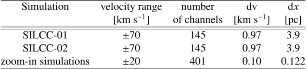
C ii ] hyperfine structure lines . . . . 72 3.2 List of the spectral and spatial resolution, dv and dx, respectively,

used in the di ff erent simulations. . . . 79 3.3 Peak intensities and luminosities of the synthetic [

C ii ] and [

C ii ]

line emission maps for the SILCC-01 and SILCC-02 simulations. . . 84 3.4 List of the peak intensities and luminisities of the [C ii ] emission

lines for MC2. . . . 85 4.1 Peak intensities and luminosities of the run S10-KS-rand at t =

50 Myr, testing di ff erent escape probability lengths L

. . . . 88 4.2 List of the peak intensities and luminosities in the synthetic [

C ii ]

emission maps for S10–KS–rand at t = 50 Myr, assuming di ff erent microturbulences. . . . 91 4.3 Summary of the luminosities and peak intensities of the [

C ii ] and

[

C ii ] line emission, analysed for the zoom-in simulations at dif- ferent resolutions. . . . 98 4.4 List of the resolution levels used for the simulation of a spherical

molecular cloud as a test setup. . . 107 4.5 Same as Table 4.4, but for the test setup of a molecular cloud at

higher densities (see text). . . . 110 5.1 Peak intensities and luminosities of the synthetic [

C ii ] line emis-

sion maps for the run S10–KS–rand at di ff erent times. . . 115 5.2 Peak intensities and luminosities of the synthetic [

C ii ] line emis-

sion maps as well as the maximum average intensities I

for the vertical profiles for the SILCC-01 and SILCC-02 simulations. . . . 120 5.3 Summary of the chosen distances and the resulting spatial reso-

lutions for the convolution of the synthetic maps with a Gaussian beam of θ

= 11.5

. . . . 122

23

24 L ist of T ables 6.1 Summary of the parameter space of the [C ii ] emitting gas, analysed

for the SILCC-01 and SILCC-02 simulations . . . 133 6.2 List of the parameters characterizing the [C ii ] line emitting gas,

analysed with the [

C ii ] line emission . . . 146 6.3 List of the parameters characterizing the [C ii ] line emitting gas,

analysed with the [

C ii ] line emission . . . 151 6.4 List of the parameters characterizing the [C ii ] line emitting gas for

MC2 at di ff erent resolutions, analysed with the [

C ii ] line emission 153 7.1 Summary of the values of the Y

factor, quantifying the range of

Y

values. . . . 166 8.1 Parameters and Tauber values of the example line profiles from MC2.175 9.1 List of the frequencies for the complementary data in H i , and the

CO lines . . . 190 9.2 List of the peak intensities of the H i emission lines for S10–KS–

rand and MC2 for di ff erent assumptions, and the luminosities of the maps. . . 194 9.3 List of the peak intensities and luminosities of the CO emission

lines for MC2. . . 201

1 List of constants. . . 229

2 List of physical quantities used in this work. . . 230

3 List of abbreviations used in this work. . . 231

Preamble

Everything is about time. The time that we have on Earth is a gift. To use it in the way we want, a pleasure. To struggle with it, exhausting. It turns back to pleasure, whenever we realise that time is a gift. Dear reader, I wish that you have the chance to experience this. This time is yours, use it as yours.

If you wish, you can take the time to learn about the things in the Universe.

About star forming regions, about molecular clouds. I used the last four years to investigate where the [C ii ] line emission comes from.

“What is that?” You may ask with interest.

It is the fine structure emission line that we observe from carbon ions. If we could see the interstellar medium at wavelengths of λ = 157.74 µm, we would see it as a bright disc. And that is made up of molecular clouds, where stars will form.

The even brighter regions are those clouds that already contain stars. The stars heat the gas in their surrounding, and this ionizes even more carbon atoms. Layers dominated by photons form whenever the radiation penetrates regions of dense gas.

We call them “photon dominated regions” (PDRs). The photons ionize the gas.

Therefore, the PDRs contain a large amount of carbon ions, so that they are bright in the [C ii ] line emission.

“How do you know about the [C ii ] line emission?” You might ask with interest.

We need instruments to see the [C ii ] line. We sent balloons with instruments into the sky to look above the blanket of atmosphere, that blocks the emission before it reaches Earth’s surface. We take planes to fly a bit higher and to see [C ii ] more precisely. We sent rockets up into space to come more close to the objects we study.

“Is this what you are doing?” You ask.

No. We started being fascinated by the observations. And we want to understand the interplay of the gas in the interstellar medium exposed to di ff erent environments.

That is why we started building models. We combine what we know about flowing gas, what we know about the chemistry within the gas. Sometimes we even let it interact with magnetic fields. We tell all this to the computer and ask the computer to tell us the story about the scenario we just described with maths. And then we get a story in the form of a simulation. I take these stories and try to interpret them.

I ask another program to predict how the scenario looks like in the light of the [C ii ] line emission. And this I take for doing my analysis.

“What do you analyse?”

We want to understand more precisely the origin of the [C ii ] line emission. We first need to understand this in our models. We then want to help interpreting the observations, and see whether the [C ii ] line emission can be used to count stars or estimate the dark gas in the interstellar medium. We are curious how the [C ii ]

25

26 P reamble

emission is distributed. This work builds up on answer to these questions. I invite

you to read this book.

1

Introduction

To ponder on the nature of the world in which we live, is probably one of the fun- damental questions that occupies humans. One aspect of this is to wonder about the things that exist beyond the Earth, the things that we call the Universe. Throughout history people have used the methods they had to study the world around the Earth.

With the naked eye one can see the stars, and if the night is dark enough, identify the Milky Way on the sky, which, as we learned, is the Galaxy that we live in. Nowa- days, we build instruments to observe the Universe with a better resolution than our eyes, and at wavelengths outside the visible spectrum. With the information we gained, our picture of the Universe has changed. By studying it in more detail, we aim to build a consistent picture of the Universe; in the past we understood it in a framework of stories and mythology; nowadays our story is written in science.

1.1 The Milky Way

The Milky Way consists of a thick and a thin disc of stars, and a concentration of gas and dust in an extreme disc (Buser, 2000). In its centre is a bulge, hosting a black hole. The Milky Way is embedded in a halo of stars, and a halo of dark mat- ter. A sketch of it is presented in Fig. 1.1, taken from Buser (2000, fig. 1 therein).

The halo consists of stars and tenuous gas, with a radius of about ∼100 kpc (Buser, 2000). The stars in the halo belong to an older population compared to the stars in the disc (Weigert et al., 2016). The disc components have a radius of ∼15 kpc.

The total mass of the Milky Way within that radius is expected to be ∼ 10

M , distributed in stars (∼ 5 × 10

M ), dark matter (∼ 5 × 10

M ), and interstellar gas (∼ 7 × 10

M Draine, 2011). Seen from our perspective on Earth, we experience the Milky Way as a bright band of emission. A view of the Milky Way at di ff erent

27

28 C hapter 1. I ntroduction

Figure 1.1: Sketch of the composition of the Milky Way, taken from Buser (2000), fig. 1 therein. The Milky Way consist of a thin and a thick disc, with a concentration of gas and dust in the extreme disc, and a bulge in the galactic centre. The Milky Way is embedded in a halo of stars and dark matter. The direction of the north and south galactic poles are indicated with NGP and SGP, respectively.

Figure 1.2: The Milky Way, seen with the Planck satellite in a wavelength range of 30 to 857 GHz, thus detecting the emission from gas and dust in the galactic plane.

The contours indicate the CO emission (Dame et al., 2001), used to identify molecular

clouds (credit: ESA, footnote 1).

C hapter 1. I ntroduction 29 wavelengths is shown in Fig. 1.2 (credit: ESA

). The Milky Way is not an isolated system. The Milky Way might interact with its closest neighbours: the Small and Large Magellanic clouds (SMC, LMC), or the Andromeda Galaxy M31. These are marked in Fig 1.2.

The disc consists of stars and the gas and dust between the stars, called the in- terstellar medium (ISM). Its structure shows spiral arms. The gas in the disc is com- posed of atomic, molecular, and ionized gas. These components are not equally dis- tributed, neither in the vertical nor horizontal dimension, but are commonly found in well separated stable phases. The molecular gas peaks at a molecular ring at a radius of ∼ 4.5 kpc. Atomic gas, on the other hand, has a flat distribution, and dominates in the outer part of the Milky Way (Tielens, 2005). Although there is no sharp boundary of the Galaxy, its dimension can be estimated by observations of its gas and star components. Considering the gas measured in atomic hydrogen (H i ) or transition lines of CO, the radius of the Milky Way is about 15 kpc, and its thickness, as defined as the point when the density of the gas drops by 50%, is about z

≈ 250 pc. Since the vertical height is much smaller than the radius, the disc is called “thin / disc” (Draine, 2011). Our solar system is positioned at a radius of ∼ 8.5 kpc from the centre of the Galaxy. In addition, there are observational indications e.g. of H i and CO (May et al., 1993, Dickey & Lockman, 1990) and of the stellar component (Carney & Seitzer, 1993, Momany et al., 2006), that the galactic disc is warped.

As habitants of the Milky Way it is challenging to get a concrete picture of our own Galaxy. However, there are other galaxies found with Milky Way like proper- ties. Two such examples, shown in Fig. 1.3, are the galaxy NGC 891 seen edge-on

, while NGC 1232 is seen face on

(Hughes et al., 2015, Weigert et al., 2016). The galaxy NGC 891 has a distance of ∼ 9.77 Mpc (Karachentsev et al., 2004), and thought to be similar to the Milky Way with respect to its morphology and physi- cal properties (Madden et al., 1994). It has a size of 13.1

, which corresponds to a physical size of ∼ 37 kpc at its distance. NGC 1232 is at a distance of ∼ 22 Mpc, with a diameter of about ∼ 43 kpc, which is almost twice the diameter of the Milky Way (M¨ollenho ff et al., 1999, Nasonova et al., 2011).

1.2 The interstellar medium

The interstellar medium consist of gas and dust, with a gas to dust mass ratio of roughly 100. The gas in the ISM of the Milky Way consists of ∼73% hydrogen and

1

This picture is taken from http://sci.esa.int/planck/47341-selected- galactic-and-extragalactic-sources-in-the-microwave-sky-as-seen-by-planck/

(credit:ESA).

2

The picture is taken from https://www.spektrum.de/alias/wunder-des-weltalls/

ngc-891-in-der-andromeda/1551412 (credit: Franz Klauser)

3

The picture is taken from https://www.eso.org/public/germany/images/

eso9845d/(credit: ESO)

30 C hapter 1. I ntroduction

Figure 1.3: Presentation of the Milky Way like galaxies NGC 891 (left, credit: Franz Klauser, footnote 2) and NGC 1232 (right, credit: ESO, footnote 3). The picture of NGC 1232 is composed of three individual pictures, showing the ultraviolet, blue, and red light. In the centre of NGC 1232, there are old, red stars, while in the spiral arms mostly young, blue stars are present.

∼27% helium. Elements with an atomic number of Z ≥ 3 contribute to about ∼1%, but have a great impact on the chemistry in the gas (Draine, 2011).

1.2.1 Processes in the ISM

Depending on the density, temperature and composition of the gas, it is heated and cooled by di ff erent processes. We describe here shortly the important processes for the di ff erent regimes of the gas.

Heating in the ISM

Di ff erent processes yield to the heating of the gas. Their contributions can be sum- marized in a heating rate Γ , which measures how much energy (in erg) and time (in s

) is transferred to the gas. In general, the coupling of radiation to the ISM is the dominant heating source. There are contributions from synchrotron emission, the cosmic microwave background, infrared (IR) emission from dust, and from stars, with O- and B-type stars producing ultraviolet (UV) and far-UV radiation. In the proximity of stellar sources, the contribution from the stars dominates. All contri- butions can be summarized in an interstellar radiation field (ISRF). The strength of the UV radiation field is often expressed in units of G

, which is the Habing field defined as G

= 1.2 × 10

erg cm

s

sr

(Habing, 1968, Tielens, 2005).

Radiation can cause photoionization or the photoelectric e ff ect in gas and dust

(Tielens, 2005). The energy of the radiation is then transferred to thermal energy

C hapter 1. I ntroduction 31 of the reaction products, which is the electron and a remaining charged particle.

Further energy transfers can happen via elastic collisions. Photons with energies hν ≥ 13.6 eV can ionize hydrogen. In an energy range of 11.2 eV ≤ hν ≤ 13.6 eV, carbon is ionized. Photons with even lower energies, 5 eV ≤ hν ≤ 11.2 eV, in- teract with polycyclic aromatic hydrocarbon molecules (PAHs) and dust grains by the photoelectric e ff ect. Likewise, the radiation can interact with molecules. They can cause photodissociation of molecules, such as H

. This process is important in atomic and molecular gas. The absorption of an UV photon can excite H

to a higher electronic state. This can decay to a vibrational excited electronic ground state, while the energy di ff erence is transferred to the surrounding gas. Via collision or emission of radiation, the vibrational excited state can further decay. This pro- cess is called vibrational heating (Stahler & Palla, 2005). Further, if gas and dust are well coupled, interactions between dust and gas particles can take place. If the tem- perature of the gas is lower than the temperature of the dust, the interaction of gas particles bouncing o ff a dust grain results into the heating of the gas (Tielens, 2005).

Interactions of gas and dust with cosmic rays lead to heating. Cosmic rays are charged, relativistic protons, with an admixture of heavy elements and elec- trons with energies in the range of 10 to 10

MeV (Tielens, 2005). Cosmic rays with energies below 10

MeV are believed to originate from particle accelerations within the magnetized shocks created by supernova remnants. Cosmic rays with even higher energy are probably extragalactic in origin (Stahler & Palla, 2005).

Cosmic rays can interact with molecular hydrogen by exciting it to a higher elec- tronic state, that leads to dissociation. H

is ionized in this process, providing a secondary electron that can further interact with the gas, e.g. by ionizing the gas, or by scattering, which can yield to the excitation of another H

molecule. In a similar manner, atomic hydrogen can be ionized by cosmic rays, producing a secondary electron, that in turn can interact with the gas (Stahler & Palla, 2005).

Heating can also occur due to mechanical processes in the ISM (Tielens, 2005).

Gravitational contraction of a dense cloud is one example, where the compression of the gas results in an increase of the temperature. This is important in the collapse phase of molecular cloud cores. Movements within the gas can contribute to the heating. If the gas is partially ionized, the influence of magnetic fields can yield to a small velocity di ff erence between the ions and neutrals in the gas. The movement of neutrals and ions then cause friction, that heats the gas. This process is called ambipolar di ff usion. Further, the ISM is turbulent. Following the theory of Kol- mogorov (1941), turbulence is injected on large spatial scales, and decays towards smaller scales. On the dissipation length scale, which is determined by the viscos- ity of the ISM, the energy is converted into heat. Additionally, shock waves convert supersonic motion into heat. A source for those shocks are SN explosions (Tielens, 2005).

Di ff erent heating processes dominate at di ff erent density ranges of the gas. In

the ionized medium, the heating is dominated by photons with high energies (≥ 13.6 eV),

that cause the ionization of atomic hydrogen. In the atomic medium, the photo dis-

sociation of small molecules is important for the heating of the gas. This process

32 C hapter 1. I ntroduction can take place if dense gas is illuminated by strong far-UV fields. In the warm neu- tral medium the photo-electric e ff ect is dominant at high densities, while the heating due to cosmic rays and X-rays are important at high densities. In the dense medium, cosmic rays can penetrate the gas, and their influence is important for the heating of this gas.

Cooling in the ISM

The gas of the ISM looses energy when photons from its constituents are emitted.

Although the abundance of species with Z > 2 is about 1% of the mass, line tran- sitions in these atoms, and the molecules formed from these elements have a large impact on the cooling of the gas. Hydrogen and helium act as important collisional partners for the heavier species and dust grains, exciting internal degrees of freedom (Stahler & Palla, 2005). According to the chemical composition of the gas, which is dependent on the gas temperature and density, molecules, atoms, or ions, their interaction with electrons, and dust contribute to the cooling of the gas.

In ionized gas, cooling dominantly takes place due to the excitation of low-lying electronic states of heavy ions, such as O

or N

, resulting in their fine-structure transition. Ions can contribute to the cooling by recombining with electrons. In such a free-bound transition the electron looses energy by emitting a photon. Charged particles in the gas interact via the Coulomb force, and by this emitting a photon.

This emission is called bremsstrahlung or free-free emission (Tielens, 2005). Ion- ized hydrogen contributes to the cooling of the gas by free-bound and free-free transitions.

The atomic gas phase is mainly cooled by fine structure transitions in C

or in O. To excite these species to the higher electronic level, H and H

are important collisional partners in the denser gas regions. However, since some species like carbon, sulphur, or siliceous (C, S, Si) have an ionization potential below 13.6 eV, there exist also free electrons in the atomic gas phase, so that collisions with these can likewise excite C

or O (Stahler & Palla, 2005, Tielens, 2005). Further, atomic hydrogen can be excited. A transition to its ground state takes then place by emit- ting a Lyman α photon. This process is called Lyman-α cooling (Tielens, 2005).

In the molecular gas, carbon and oxygen no longer exist separately, but form CO. Due to collisions, the rotational levels of CO are excited, and a transition to the ground state takes place by emitting a photon. Since the lower lying CO rotational transitions of carbon are optically thick, the emitted photons are trapped within the molecular gas, moving via di ff usion, and only escape at the cloud surface (Stahler

& Palla, 2005). Further cooling takes place due to interaction of the gas with dust grains. Collisions between the gas and the dust grains reduce the kinetic energy of the gas, and result in lattice vibrations of the dust, that decay by the emission of a photon. These photons contribute to the infrared continuum emission (Tielens, 2005).

To measure the cooling of the gas, a cooling rate Λ is used, which expresses

C hapter 1. I ntroduction 33

Figure 1.4: Interstellar cooling function Λ(x, T ) , as presented in Dalgarno & McCray (1972) in their fig. 2 (left). The fractional ionization is denoted by x , and indicated at each line. The right panel shows the cooling curve with the contribution from the different elements as presented by Gnat & Ferland (2012), fig. 3 therein.

how much energy (in erg), integrated over a certain volume element (in cm

), is transferred to the environment over time (in s

). The processes described above can be summarized in cooling curves, as done in e.g. Dalgarno & McCray (1972), Sutherland & Dopita (1993) and Gnat & Ferland (2012). Figure 1.4 shows the cool- ing curve for the atomic gas phase as a function of the temperature in the optically thin limit. In the left panel the curve is presented for a larger range of tempera- tures between 10 K and 10

K. The di ff erent lines indicate the cooling curves for di ff erent degrees of ionization in the gas. For T ≤ 10

K the gas is mainly cooled by fine structure transitions. Depending on the degree of ionization in the gas, the e ffi ciency in the cooling changes.

The right panel of Fig. 1.4 shows the contribution from the di ff erent elements

to the cooling curve for T & 10

K. It is assumed that the gas is in collisional ion-

ization equilibrium. At temperatures of T ∼ 2 × 10

K, cooling is dominated by

hydrogen Lyman-α cooling. Carbon cools most e ffi cient at T ∼ 10

K, followed

by oxygen at T ∼ 3 × 10

K. Further, cooling by neon (T ∼ 5 × 10

K) and iron

(T ∼ 1.5 × 10

K and 10

K) takes over. As fewer electrons are bound to their

atoms, the less e ffi cient the cooling becomes, so that the cooling curve drops above

10

K (Tielens, 2005). For temperatures larger than 10

K, the cooling is dominated

by thermal bremsstrahlung due to the fully stripped ions (Gnat & Ferland, 2012,

Tielens, 2005).

34 C hapter 1. I ntroduction

Figure 1.5: Schematic representation of the equilibrium curve ( Λ /(kT ) ), illustrating the resulting two phases of the ISM (credit: Tielens, 2005, , fig. 8.1 therein, taken from Shull et al. 1987). Above the curve, heating exceeds cooling, and below the curve, cooling dominates. The horizontal line indicates a constant heating rate and constant pressure.

The intersection points of the cooling curve with the horizontal line are the equilibrium points, from which two are stable and two are unstable, so that multiple phases coexist.

1.2.2 Phases of the ISM

Although one might expect the gas to be present at any region in the temperature- density phase space, most of it is constrained to narrow temperature-density regions, known as the phases of the ISM. These phases are determined by the balance be- tween the cooling, Λ , and heating, Γ , which can be expressed in

L = n

Λ − n Γ . (1.1)

Given that heating and cooling depend on the density and temperature of the gas, it is possible to find conditions of temperature and density, where L = 0. This is also known as the equilibrium curve. As a consequence of this equilibrium curve, the two phase model of the ISM is derived. A schematic illustration is shown in Fig. 1.5.

In that model, the phases of the cold neutral medium (CNM), forming the molecular clouds, and the warm neutral medium (WNM) and warm ionized medium (WIM), present in the intercloud gas, coexist in thermal and pressure equilibrium. For these assumption the two-phase model predicts the CNM at temperatures around 50 K and number densities around 60 cm

, and a WNM with T ∼ 7500 K and n ∼ 0.4 cm

(Tielens, 2005).

Caused by supernova (SN) explosions turbulent energy is injected to the ISM,

and the gas is heated. This results in the formation of an additional very hot, and

C hapter 1. I ntroduction 35 tenuous gas phase, with T ∼ 10

K and n ∼ 10

cm

. This is the hot intercloud medium, or hot ionized medium (HIM), present in a SN driven ISM. Due to its low density, the radiative cooling does not work e ffi ciently in this gas phase. Thus, it co- exist with the CNM, WNM and WIM, but is not in thermal equilibrium. The HIM, WNM and WIM, and CNM together build the three-phase model of the ISM, also called McKee-Ostiker model (McKee & Ostriker, 1977). The CNM is expected to mainly exist in the galactic disc, but might extend to some distance from the disc midplane due to the turbulent cloud velocity dispersion. The HIM, WNM and WIM are expected to form the low halo, while the HIM is found towards higher latitudes (Tielens, 2005).

There are di ff erent schemes to classify the gas phases in greater detail. Draine (2011) distinguishes between the following phases:

• Coronal gas (or hot ionized medium, HIM), which is shock-heated gas, mostly ionized and with T ≥ 10

K and n

∼ 0.004 cm

.

• H ii gas, which predominantly forms around massive O-type stars. These stars emit photons in the ultraviolet regime, that ionize hydrogen. This gas is at temperatures of T ∼ 10

K and densities n

between 0.2 and 10

cm

.

• Warm H i gas (or warm neutral medium, WNM), which is mostly atomic gas, with T ∼ 5 × 10

K and n

∼ 0.6 cm

.

• Cool H i gas (or cool neutral medium, CNM), is likewise atomic gas, but at lower temperatures of T ∼ 100 K and higher densities of n

∼ 30 cm

.

• Di ff use H

gas, in which the shielding in the gas is su ffi cient that H

can form.

This gas has temperatures of T ∼ 50 K and densities of n

∼ 100 cm

.

• Dense H

gas, with T between 10 and 50 K and n

between 10

and 10

cm

, which forms gravitationally bound clouds. In those clouds stars can form.

An alternative, more simplified classification is provided in Mihalas & Binney (1981), and used in Walch et al. (2015). Here, the gas is distinguished between

• hot gas, mostly from SN remnants (T ≥ 3 × 10

K),

• warm-hot, ionized gas (8 × 10

K < T < 3 × 10

K),

• warm atomic and partly ionized gas (300 K ≤ T ≤ 8 × 10

K),

• thermally stable cold gas (T < 300 K),

• very cold and dense gas, most likely in molecular form (T < 30 K).

1.2.3 Molecular clouds

Molecular clouds are characterized by their higher densities and thus, lower temper-

atures compared to the embedding material. The classification of molecular clouds

into groups has no strict limits. However, one approach is to distinguish the molecu-

lar clouds by its visual extinction A

(Stahler & Palla, 2005, Snow & McCall, 2006,

Draine, 2011):

36 C hapter 1. I ntroduction

• Clouds with a low visual extinction (A

∼ 1) are “di ff use clouds”. They have typical total gas number densities between ∼100 and 500 cm

, temperatures around T ∼ 50 K, and masses of M ∼ 50 M . Their sizes are about 3 pc.

• Translucent molecular clouds have a slightly larger visual extinction (A

∼ 2), typical number densities of 500 to 5000 cm

, and temperatures of 10 to 50 K (Snow & McCall, 2006).

• Clouds with masses of M ∼ 10

M , visual extinction of A

& 2, on scales of L ∼ 50 pc can be classified as “giant molecular clouds” (GMC). They have number densities of about n ∼ 100 cm

, and temperatures about T ∼ 15 K.

• Clouds with visual extinctions around A

∼ 5 are dark clouds. They have smaller dimensions compared to the GMCs (L ∼ 10 pc), and smaller masses (M ∼ 10

M ), while their total number densities are around n ∼ 500 cm

, and the temperatures of T ∼ 10 K are slightly smaller than in GMCs.

• Due to gravitational collapse in molecular clouds, dense cores can form.

These are of small dimension (L ∼ 0.1 pc), and have visual extinctions of A

∼ 10. Their number densities are about n ∼ 10

cm

, and their tempera- tures are about T ∼ 10 K. It is within these cores where star formation takes place.

• Infrared dark clouds are characterized by a high visual extinction of A

∼ 10 to 100, so that they are opaque even at 8 µm (Draine, 2011).

As a result of the shielded gas, the intensity of the far-UV radiation is reduced within molecular clouds, and the gas-phase chemistry is mainly driven by cosmic ray ionization (Tielens, 2005). Due to the low temperatures, atoms and molecules from the gas phase freeze out on the surface of dust grains, forming an ice man- tle around them. Thus, chemical species and molecules are depleted from the gas phase. This changes the chemistry in the gas phase, as well as introduces the ice as a further chemical reaction component, since now interaction between the gas phase and the solid state takes place (Tielens, 2005).

In dense regions molecular clouds can gravitationally collapse and from proto- stars, whose feedback likewise influences the energy balance of the gas as well as its chemical composition. Massive stars (O- and B-type) can influence the ISM by stellar winds, and their radiation. A typical GMC survives around 3 × 10

yr, before it is destroyed by the winds of its stars (Stahler & Palla, 2005). Further, the UV radiation of the embedded stars evaporate the ice mantles of the dust grains and ion- ize the surrounding gas. In the transition regions from the ionized to the molecular gas phase, photon-dominated regions (PDRs) evolve (Hollenbach & Tielens, 1999).

The far-UV radiation (6 eV < hν < 13.6 eV) from the stars is no longer su ffi cient to ionize hydrogen, but it still dominates the chemistry of the gas and ionizes species with ionization potentials below that of hydrogen. Carbon is one species, that be- comes ionized in those PDRs. Thus, PDRs are observable in the emission line from C

, which is a fine structure emission line [C ii ].

Often, the molecular clouds do not exist in isolation, but form large cloud com-

plexes. In galaxies, these are situated within the galactic disc. In Fig. 1.2 the con-

tours mark emission from the

CO (1–0) line, indicating the molecular clouds. One

example is Orion, shown in Fig. 1.6 (Kong et al., 2018, fig. 5 therein), which is a

C hapter 1. I ntroduction 37

Figure 1.6: Orion molecular cloud in the integrated

CO (1–0) intensity (over the veloc-

ity range of 2.5 - 15 km s

), as presented by Kong et al. (2018), fig. 5 therein.

38 C hapter 1. I ntroduction

Figure 1.7: Taurus molecular cloud complex, as presented in Goldsmith et al. (2008) in fig. 14 therein. The grey colours show the H

column density. The symbols mark the position of the stars. Diamonds indicate diffuse, extended sources, squares indicate Class I or younger stars, asterisks indicate T Tauri stars (see Goldsmith et al., 2008).

star forming molecular cloud complex at a distance of 450 pc (Genzel & Stutzki, 1989). It contains OB-type stars, and thus, it is suitable to study the formation of stars, filaments, and the influence of stellar feedback on the ISM. Due to its active star formation, Orion is also used to study the chemistry and structure of PDRs (e.g.

Andree-Labsch et al., 2017).

Another example is Taurus, a well studied molecular cloud (Goldsmith et al., 2008), situated in our proximity, with a distance of about ∼140 pc (∼126 pc), ac- cording to Elias (1978) (Hartigan & Kenyon, 2003, respectively). A study of the region within a field of 100 deg

in

CO and

CO rotational transition J = 1 − 0 was done by Goldsmith et al. (2008). Figure 1.7 shows the Taurus molecular cloud complex (Goldsmith et al., 2008, fig. 14 therein). Assuming that Taurus is at a distance of about 140 pc, (10 deg)

correspond to ∼(24 pc)

. They find a com- plex structure of the molecular cloud, with filaments, ridges, blobs, and holes.

They estimate the mass of Taurus with their observations, and find a mass of about 2.35× 10

M . Half of this mass is present in regions with total gas column densities N ≤ 2.1 × 10

cm

. Star formation takes place in Taurus since about 10 Myrs, where most of the stars were formed during the last 3 Myrs (Palla & Stahler, 2002, Goldsmith et al., 2008).

Regions of molecular cores in infrared dark clouds (IRDC) and cold, massive, molecular clouds were studied with Herschel as part of the Earliest Phases of Star Formation (EPOS) key program (Ragan et al., 2012). They analysed with the Her- schel PACS

instrument the emission at 70, 100, and 160 µm, and with SPIRE the

4

PACS stands for Photoconductor Array Camera and Spectrometer, and is an instrument onboard

Herschel.