Mondshein Sequences (a.k.a. (2, 1)-Orders)

Mondshein Sequences (a.k.a. (2, 1)-Orders)

Jens M. Schmidt Institute of Mathematics

TU Ilmenau

Abstract

Canonical orderings [STOC’88, FOCS’92] have been used as a key tool in graph drawing, graph encoding and visibility representations for the last decades. We study a far-reaching generalization of canonical orderings to non-planar graphs that was published by Lee Mondshein in a PhD-thesis at M.I.T. as early as 1971.

Mondshein proposed to order the vertices of a graph in a sequence such that, for any

, the vertices from 1 to

induce essentially a 2-connected graph while the remaining vertices from

+ 1 to

induce a connected graph. Mondshein’s sequence generalizes canonical orderings and became later and independently known under the name

. Surprisingly, this fundamental link between canonical orderings and non-separating ear decom- position has not been established before. Currently, the fastest known algorithm for computing a Mondshein sequence achieves a running time of

(

); the main open problem in Mondshein’s and follow-up work is to improve this running time to subquadratic time.

After putting Mondshein’s work into context, we present an algorithm that computes a Mondshein sequence in optimal time and space

(

). This improves the previous best running time by a factor of

. We illustrate the impact of this result by deducing linear-time algo- rithms for five other problems, for four out of which the previous best running times have been quadratic. In particular, we show how to

– compute three independent spanning trees in a 3-connected graph in time

(

), improving a result of Cheriyan and Maheshwari [J. Algorithms 9(4)],

– improve the preprocessing time from

(

) to

(

) for the output-sensitive data structure by Di Battista, Tamassia and Vismara [Algorithmica 23(4)] that reports three internally disjoint paths between any given vertex pair,

– derive a very simple

(

)-time planarity test once a Mondshein sequence has been com- puted,

– compute a nested family of contractible subgraphs of 3-connected graphs in time

(

), – compute a 3-partition in time

(

), while the previous best running time is

(

) due to

Suzuki et al. [IPSJ 31(5)].

1 Introduction

Canonical orderings are a fundamental tool used in graph drawing, graph encoding and visibility representations; we refer to [2] for a wealth of applications. For maximal planar graphs, canonical orderings were introduced by de Fraysseix, Pach and Pollack [9, 10] in 1988. Kant then generalized canonical orderings to 3-connected planar graphs [23, 24]. In polyhedral combinatorics, canonical

∗This research was partly done at Max Planck Institute for Informatics, Saarbrücken. An extended abstract of this paper has been published at ICALP’14.

orders are in addition related to shellings of (dual) convex 3-dimensional polytopes [42]; however, such shellings are often, as in the Bruggesser-Mani theorem, dependent on the geometry of the polytope. A combinatorial generalization to arbitrary planar graphs was given by Chiang, Lin and Lu [7].

Surprisingly, the concept of canonical orderings can be traced back much further, namely to a long-forgotten PhD-thesis at M.I.T. by Lee F. Mondshein [29] in 1971. In fact, Mondshein proposed a sequence that generalizes canonical orderings to non-planar graphs, hence making them applicable to arbitrary 3-connected graphs. Mondshein’s sequence was, independently and in a different notation, found later by Cheriyan and Maheshwari [6] under the name non-separating ear decompositions and is sometimes also called (2,1)-order (e.g., see [5]). In addition, Mondshein sequences provide a generalization of Schnyder’s famous woods to non-planar 3-connected graphs.

One key contribution of this paper is to establish the above fundamental link between canonical orderings and non-separating ear decompositions in detail.

Computationally, it is an intriguing question how fast a Mondshein sequence can be computed.

Mondshein himself gave an involved algorithm with running time O(m

). Cheriyan showed that it is possible to achieve a running time of O ( nm ) by using a theorem of Tutte that proves the existence of non-separating cycles in 3-connected graphs [36]. Both works state as main open problem, whether it is possible to compute a Mondshein sequence in subquadratic time (see [29, p.

1.2] and [6, p. 532]).

We present the first algorithm that computes a Mondshein sequence in optimal time and space O(m), hence solving the above 45-year-old problem. The interest in such a computational result stems from the fact that 3-connected graphs play a crucial role in algorithmic graph theory. We illustrate this in five applications by giving linear-time algorithms. For four of them, the previous best running times have been quadratic.

We start by giving an overview of Mondshein’s work and its connection to canonical orderings and non-separating ear decompositions in Section 3. Section 4 explains the linear-time algorithm and proves its main technical lemma, the Path Replacement Lemma. Section 5 covers five applica- tions of our linear-time algorithm.

2 Preliminaries

We use standard graph-theoretic terminology and assume that all graphs are simple.

Definition 1 ([26, 40]). An ear decomposition of a graph G = (V, E) is a sequence (P

, P

, . . . , P

) of subgraphs of G that partition E such that P

is a cycle and every P

, 1 ≤ i ≤ k , is a path that intersects P

∪ · · · ∪ P

in exactly its endpoints. Each P

is called an ear . An ear is short if it is an edge and long otherwise.

According to Whitney [40], every ear decomposition has exactly m −n +1 ears and G has an ear decomposition if and only if G is 2-connected. For any i , let G

:= P

∪· · ·∪P

and V

:= V − V ( G

).

We write G

to denote the graph induced by V

. Note that G

does not necessarily contain all edges in E − E ( G

); in particular, there may be short ears in E − E ( G

) that have both endpoints in G

. For a path P and two vertices x and y in P , let P [ x, y ] be the subpath in P from x to y . A path with endpoints v and w is called a vw-path . A vertex x in a vw -path P is an inner vertex of P if x / ∈ {v, w} . For convenience, every vertex in a cycle is called an inner vertex of that cycle.

For an ear P , let inner ( P ) be the set of its inner vertices. The inner vertex sets of the ears in

an ear decomposition of G play a special role, as they partition V . Every vertex of G is contained

in exactly one long ear as inner vertex. This readily gives the following characterization of V

.

Observation 2. For every i, V

is the union of the inner vertices of all long ears P

with j > i.

We will compare vertices and edges of G by their first occurrence in a fixed ear decomposition.

Definition 3. Let D = (P

, P

, . . . , P

) be an ear decomposition of G. For an edge e ∈ G, let birth

( e ) be the index i such that P

contains e . For a vertex v ∈ G , let birth

( v ) be the minimal i such that P

contains v (thus, P

is the ear containing v as an inner vertex). Whenever D is clear from the context, we will omit D.

Clearly, for every vertex v , the ear P

is long, as it contains v as an inner vertex.

3 Generalizing Canonical Orderings

Although canonical orderings of (maximal or 3-connected) planar graphs are traditionally defined as vertex partitions, we will define them as special ear decompositions. This will allow for an easy comparison of canonical orderings to the more general Mondshein sequences, which extend them to non-planar graphs. We assume that the input graphs are 3-connected and, when talking about canonical orderings, planar. It is well-known that maximal planar graphs (which were considered in [9] in this setting) form a subclass of 3-connected graphs, apart from the triangle-graph.

Definition 4. An ear decomposition is non-separating if, for every long ear P

except the last one, every inner vertex of P

has a neighbor in G

.

The name non-separating refers to the following helpful property.

Lemma 5. In a non-separating ear decomposition D, G

is connected for every i.

Proof. For all i satisfying G

= ∅ the claim is true, in particular if i is at least the index of the last long ear. Otherwise, i is such that the inner vertex set A of the last long ear in D is contained in G

. Consider any vertex x in G

. In order to show connectedness, we exhibit a path from x to A in G

. If x ∈ A , we just take the path of length zero. Otherwise, the vertex x has a neighbor in G

, since D is non-separating. According to Observation 2, this neighbor is an inner vertex of some ear P

with j > birth ( x ). Applying induction on j gives the desired path to A .

A plane graph is a graph that is embedded into the plane. In particular, a plane graph has a fixed outer face. We define canonical orderings as follows.

Definition 6 (canonical ordering) . Let G be a 3-connected plane graph and let rt and ru be edges of its outer face. A canonical ordering through rt and avoiding u is an ear decomposition D of G such that

1. rt ∈ P

,

2. P

is the last long ear, contains u as its only inner vertex and does not contain ru , and 3. D is non-separating.

The fact that D is non-separating plays a key role for both canonical orderings and their gener- alization to non-planar graphs. E.g., Lemma 5 implies that the plane graph G can be constructed from P

by successively inserting the ears of D into only one dedicated face of the current embed- ding, a routine that is heavily applied in graph drawing and embedding problems. Put simply, the second condition forces u to be “added last” in D. Further motivations are given by 3-connectivity:

If we would not restrict u to be the only vertex in P

, other vertices in the same ear could

have degree two, as the non-separateness does not imply any later neighbors for the last ear.

The condition ru / ∈ P

ensures that u has degree at least three in G (which is necessary for 3-connectivity) and will also lead to the existence of a third independent spanning tree (see Application 1 in Section 5).

We note that forcing one edge rt in P

is optimal in the sense that two edges rz and rt cannot be forced: Let W be a sufficiently large wheel graph with center vertex r and rim vertices t and z such that t and z are not adjacent. Then a canonical ordering with rt, rz ∈ P

and avoiding u does not exist, as any inner vertex on the rim-path from t to z not containing u has no larger neighbor with respect to birth , and thus violates the non-separateness.

The original definition of canonical orderings by Kant [24] states the following additional prop- erties.

Lemma 7 (further properties) . For every 0 ≤ i ≤ m − n in a canonical ordering, 4. the outer face C

of the plane subgraph G

⊆ G is a (simple) cycle that contains rt, 5. G

is 2 -connected and every separation pair of G

has both its vertices in C

, and 6. for i > 0 , the neighbors of inner ( P

) in G

are contained consecutively in C

. Further, the canonical ordering implies the existence of one satisfying the following property:

7. if |inner ( P

) | ≥ 2 , each inner vertex of P

has degree two in G − V

Properties 4–6 can be easily deduced from Definition 6 as follows: Every G

is a 2-connected plane subgraph of G, as G

has an ear decomposition. According to [34, Corollary 1.3], all faces of a 2-connected plane graph form cycles. Thus, every C

is a cycle and Property 4 follows directly from the fact that rt is assumed to be in the fixed outer face of G . Property 5 is implied by the 3-connectivity of G and Property 4. Property 6 follows from Property 4, the fact that every inner vertex of P

must be outside C

(in G ) and the Jordan Curve Theorem.

For the sake of completeness, we show how Property 7 is derived. Although it is not directly implied by Definition 6 (in that sense our definition is more general), the following lemma shows that we can always find a canonical ordering satisfying it.

Lemma 8. Every canonical ordering can be transformed to a canonical ordering satisfying Prop- erty 7.7 in linear time.

Proof. First, consider any ear P

6 = P

with |inner ( P

) | ≥ 2 such that an inner vertex x of P

has a neighbor y in G − V

that is different from its predecessor and successor in P

. Then P

= xy and birth(xy) > i. If y is in P

, let Z be the path obtained from P

by replacing P

[x, y] ⊆ P

with xy ; we call this latter operation short-cutting . We replace P

with the two ears Z and P

[ x, y ] in that order and delete P

= xy . This preserves Properties 1–3 (note that u / ∈ P

, as

|inner(P

) | ≥ 2) and therefore the canonical ordering. If y is not in P

, let Z

be a shortest path in P

from an endpoint of P

to x and let Z

be the path in P

from x to the remaining endpoint.

Replace P

with the two ears Z

∪ xy and Z

in that order and delete P

. This preserves Properties 1–3.

Now, consider a vertex x ∈ P

not having degree 2 in G − V

, i.e. x has a non-consecutive neighbor y in P

in the graph that is vertex-induced by V ( P

). If x ∈ {r, t} , we replace P

with the shortest cycle C in P

∪ xy that contains r, t and y, delete P

= xy and add the remaining path from x to y in P

− E ( C ) as new ear directly after C . This clearly preserves Properties 1–3.

If x / ∈ {r, t} , we can shortcut P

in a similar way. The above operations can be computed in linear total time.

Our definition of canonical orderings uses planarity only in one place: tr ∪ ru is assumed to be

part of the outer face of G . Note that the essential part of this assumption is that tr ∪ ru is part of

some face of G, as we can always choose an embedding for G having this face as outer face. Hence,

there is a natural generalization of canonical orderings to non-planar graphs G : We merely require rt and ru to be edges of G ! The following ear-based definition is similar to the one given in [6] but does not need additional degree-constraints.

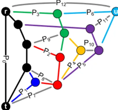
Definition 9 ([29, 6]). Let G be a graph with edges rt and ru. A Mondshein sequence through rt and avoiding u (see Figure 1) is an ear decomposition D of G such that

1. rt ∈ P

,

2. P

is the last long ear, contains u as its only inner vertex and does not contain ru, and 3. D is non-separating.

This definition is in fact equivalent to the one Mondshein used 1971 to define a (2,1)-sequence [29, Def. 2.2.1], but which he gave in the notation of a special vertex ordering. This vertex ordering actually refines the partial order inner ( P

) , . . . , inner ( P

) by enforcing an order on the inner vertices of each path according to their occurrence on that path (in any direction). The statement that canonical orderings can be extended to non-planar graphs can also be found in [14, p.113], however, no further explanation is given.

P

8

P⁷

P6

P¹¹ P₃

P2

P9

P0

P¹ r

t

u

P₁₀

P⁴ P⁵ P₁₂

Figure 1: A Mondshein sequence of a non-planar 3-connected graph.

Note that Definition 9 implies u / ∈ P

, as P

6 = P

, since P

contains only one inner vertex. As a direct consequence of this and the fact that D is non-separating, G must have minimum degree at least 3 in order to have a Mondshein sequence. Mondshein proved that every 3-connected graph has a Mondshein sequence. In fact, also the converse is true.

Theorem 10 (compare also [6, 41]) . Let rt and ru be edges of G. Then G is 3 -connected if and only if G has three internally vertex-disjoint paths between t and u and a Mondshein sequence through rt and avoiding u.

We state two additional facts about Mondshein sequences. For the first, let G be planar. Clearly, every canonical ordering of an embedding of G is also a Mondshein sequence. Conversely, let D be a Mondshein sequence of G through rt and avoiding u . Then Theorem 10 implies that G is 3-connected. If G has an embedding in which tr ∪ ru is contained in a face, we can choose this face as outer face and get an embedding of G for which D is a canonical ordering. This embedding must be unique, as Whitney proved that any 3-connected planar graph has a unique embedding (up to flipping) [39]. Otherwise, there is no embedding of G such that tr ∪ ru is contained in some face. Since the faces of a 3-connected planar graph are precisely its non-separating cycles [36], we conclude the following observation.

Observation 11. For a planar graph G and edges tr and ru, the following statements are equiva-

lent:

• There is a planar embedding of G whose outer face contains tr ∪ ru, and D is a canonical ordering of this (unique) embedding through rt and avoiding u.

• D is a Mondshein sequence through rt and avoiding u, and tr ∪ ru is contained in a non- separating cycle of G.

For the second fact, let a chord of an ear P

be an edge in G that joins two non-adjacent vertices of P

. Note that the definition of a Mondshein sequence allows chords for every P

. Once having a Mondshein sequence, one can aim for a slightly stronger structure. Let a Mondshein sequence be induced if P

is induced in G and every ear P

6 = P

has no chord, except possibly the one joining the endpoints of P

. It has been shown [6] that every Mondshein sequence can be made induced. The following lemma shows the somewhat stronger statement that we can always expect Mondshein sequences to satisfy Property 7.7. In fact, its proof is precisely the same as the one for Lemma 8, since none of its arguments uses planarity.

Lemma 12. Every Mondshein sequence can be transformed into a Mondshein sequence D satisfying Property 7.7 in linear time. In particular, D is induced.

4 Computing a Mondshein Sequence

Mondshein gave an involved algorithm [29] that computes his sequence in time O ( m

). Indepen- dently, Cheriyan and Maheshwari gave an algorithm that runs in time O ( nm ) and which is based on a theorem of Tutte. At the heart of our linear-time algorithm is the following classical construction sequence for 3-connected graphs due to Barnette and Grünbaum [3] and Tutte [37, Thms. 12.64 and 12.65].

Definition 13. The following operations on simple graphs are BG-operations (see Figure 2).

(a) vertex-vertex-addition : Add an edge between two distinct non-adjacent vertices

(b) edge-vertex-addition : Subdivide an edge ab , a 6 = b , with a vertex v and add the edge vw for a vertex w / ∈ {a, b}

(c) edge-edge-addition : Subdivide two distinct edges (the edges may intersect in one vertex) with vertices v and w , respectively, and add the edge vw

v w

v

w (a) vertex-vertex-addition

a b a b

w w

v

(b) edge-vertex-addition

a

c

b

d a

c

b

d v

w (c) edge-edge-addition

Figure 2: BG-operations

Theorem 14 ([3, 37]) . A graph is 3-connected if and only if it can be constructed from K

using BG-operations.

Hence, applying a BG-operation on a 3-connected graph preserves it to be simple and 3- connected. Let a BG-sequence of a 3-connected graph G be a sequence of BG-operations that constructs G from K

. It has been shown that such a BG-sequence can be computed efficiently.

Theorem 15 ([31, Thms. 6.(2) and 52]) . A BG-sequence of a 3 -connected graph can be computed

in time O(m) .

The outline of our algorithm is as follows. Assume we want a Mondshein sequence of G through rt and avoiding u . We will first compute a suitable BG-sequence of G using Theorem 15 and start with a Mondshein sequence of its first graph, the K

. The crucial part is then a careful analysis that a Mondshein sequence of a 3-connected graph can be modified to one of G

, where G

is obtained from the former by applying a BG-operation.

In more detail, we need a special BG-sequence to harness the dynamics of the vertices r , t and u throughout the BG-sequence. A BG-sequence is determined by an (arbitrary) DFS-tree and two fixed incident edges of its root. We choose a DFS-tree with root r and fix the edges rt and ru . This way the initial K

will contain the vertex r and r will never be relabeled [30, Section 5].

However, t and u are not necessarily vertices of the K

. This is a problem, as we have to specify an edge rt and vertex u of K

which the Mondshein sequence of K

goes through and avoids, respectively, for induction purposes. Fortunately, the relation between the graphs in a BG- sequence and subdivisions of these graphs in G [30, Section 4] gives us such replacement vertices for t and u efficiently: We find vertices t and u of the initial K

such that the following labeling process ends with the input graph G in which t = t and u = u: For every BG-operation of the BG-sequence from K

to G that subdivides the edge rt or ru , we label the subdividing vertex with t or u , respectively (the old vertex t or u is then given a different label). As desired, the final t and u upon completion of the BG-sequence will be t and u. We refer to [30, Section 4] for details on how to efficiently compute such a labeling scheme.

For the K

, it is easy to compute a Mondshein sequence through rt and avoiding u efficiently.

We iteratively proceed to a Mondshein sequence of the next graph in the sequence. The following modifications and their computational analysis are the main technical contribution of this paper and depend on the various positions in the sequence in which the vertices and edges that are involved in the BG-operation can occur.

Note that any short ear xy in a Mondshein sequence can be moved to an arbitrary position of the sequence without destroying the Mondshein property, as long as both x and y are created at an earlier position. Thus, the essential information of a Mondshein sequence is its order on long ears. We will prove that there is always a modification that is local in the sense that the only long ears that are modified are the ones containing a vertex that is involved in the BG-operation.

Lemma 16 (Path Replacement Lemma) . Let G be a 3 -connected graph with edges rt and ru and let D = ( P

, P

, . . . , P

) be a Mondshein sequence of G through rt and avoiding u. Let G

be obtained from G by applying a BG-operation Γ and let rt

and ru

be the edges of G

that correspond to rt and ru in G. Then a Mondshein sequence D

of G

through rt

and avoiding u

can be computed from D using only constantly many (amortized) constant-time modifications.

We split the proof into three parts. First, we state two preprocessing routines leg () and belly () on D that will reduce the number of subsequent cases considerably. Second, we show how to modify D to D

using these routines and, third, we discuss computational issues.

From now on, let vw be the edge that was added by Γ such that v subdivides ab ∈ E ( G ) and w subdivides cd ∈ E ( G ) (if applicable). Thus, the vertex u

in G

is either u , v or w , and likewise t

in G

is either t , v or w . By symmetry, we assume w.l.o.g. that birth ( a ) ≤ birth ( b ), birth ( c ) ≤ birth ( d ) and birth ( d ) ≤ birth ( b ). Recall that {a, b} may intersect {c, d} in at most one vertex. If not stated otherwise, the birth -operator refers always to D in this section.

We need some notation for describing the modifications. Suppose P

is an ear containing an

inner vertex z. If an orientation of P

is given, let P

[, z] be the prefix of P

ending at z in this

orientation and let P

[ z, ] be the suffix of P

starting at z . Occasionally, the orientation does not

matter; if none is given, an arbitrary orientation can be taken. For paths A and B that end and

start at a unique common vertex, let A +B be the concatenation of A and B. Similarly, for disjoint

paths A and B such that exactly one endpoint x of A is a neighbor of exactly one endpoint y of B , let A + B be the path A ∪ xy ∪ B .

Of legs and bellies: We describe two preprocessing routines. These will be used on D in the next section to ensure that ab ∈ P

and cd ∈ P

(up to some special cases). Let an edge xy / ∈ P

be a leg of P

if xy 6 = ru and birth ( x ) < birth ( y ). For each such leg, P

is a long ear, xy is a short ear, and x is either not contained in P

or an endpoint of P

(see Figures 3a and 3b). In the first case, if y is not the only inner vertex of P

, orient P

such that the successor of y is also an inner vertex of P

; this will preserve the non-separateness at y for some later cases. In the latter case, orient P

toward x.

y

x

(a) A leg xy with x ∈/ Pbirth(y)

and the result of Operationleg(x, y) (dashed lines).

y x

(b) A leg xy with x ∈ Pbirth(y) and the result of Operationleg(x, y).

y x

a

(c) A bellyxywithbirth(y)>0 and the result of Operationbelly(x, y).

x y

r t

(d) A bellyxywithbirth(y) = 0 and the result of Operationbelly(x, y).

Figure 3

A leg xy of P

has the feature that it may be incorporated into P

such that the resulting sequence is still a Mondshein sequence: Let leg(x, y) be the operation that deletes the short ear xy in the sequence D and replaces the long ear P

by the two ears P

[ , y ] + x and P

[ y, ] in that order. We prove that the resulting sequence D is a Mondshein sequence.

Clearly, D is an ear decomposition. In addition, we still have rt ∈ P

, as P

did not change due to birth ( y ) > birth ( x ) ≥ 0. Since every inner vertex of the two new ears is also an inner vertex of P

, it has a neighbor in some larger ear (with respect to birth) in D; thus D is non-separating by Definition 4. Since xy 6 = ru, the last long ear in D does not contain ru. The last long ear in D may be different from the one in D if y = u , but since the replacement does not introduce any new inner vertex, it will still contain the same vertex u as only inner vertex. Hence, D is a Mondshein sequence through rt and avoiding u by Definition 9.

Let an edge xy of G be a belly of P

if birth ( x ) = birth ( y ) 6 = birth ( xy ). Then P

contains both x and y as inner vertices, but does not contain xy ; hence xy is a short ear (see Figures 3c and 3d).

For a belly xy , we can again find a Mondshein sequence that ensures xy ∈ P

. First,

consider the case birth ( y ) > 0, in which we orient P

from y to x . For this case, let belly ( x, y )

be the operation that deletes the short ear xy in the sequence D and replaces the long ear P

by the two long ears P

[ , y ] + P

[ x, ] and P

[ y, x ] in that order (see Figure 3c). For

the same reasons as before, the resulting sequence D is an ear decomposition and non-separating.

Since P

contains two inner vertices, we have birth ( y ) 6 = birth ( u ), and it follows that the last long ear in D is exactly the last long ear of D . In addition, rt ∈ P

, as P

did not change due to birth ( y ) > birth ( x ) ≥ 0. Hence, D is a Mondshein sequence through rt and avoiding u .

Now consider the case birth ( y ) = 0. The vertices x and y cut P

into two distinct paths A and B having endpoints x and y ; let A be the one containing rt . Let belly ( x, y ) be the operation that deletes the short ear xy in D and replaces P

by the two long ears A ∪ xy and B in that order (see Figure 3d). This preserves P

to be a cycle that contains rt and, thus, gives also a Mondshein sequence through rt and avoiding u . Note that both operations leg () and belly () leave the vertices u , r and t unchanged.

Modifying D to D

: We use the operations leg() and belly() for a preprocessing on the sub- divided edges ab and cd (if applicable) by Γ. Suppose first that ru / ∈ {ab, cd} ; we will solve the remaining case ru ∈ {ab, cd} later. Assume birth ( ab ) 6 = birth ( b ) and recall that birth ( a ) ≤ birth ( b ).

If birth(a) < birth(b), ab is a leg of P

and we apply the operation leg(a, b). Otherwise, birth ( a ) = birth ( b ) and we apply the operation belly ( a, b ). In both cases, this leaves a Mondshein sequence in which birth ( ab ) = birth ( b ), i.e. ab is contained in the long chain P

.

Similarly, if birth ( cd ) 6 = birth ( d ), we want to apply either leg ( c, d ) or belly ( c, d ) to obtain birth ( cd ) = birth ( d ). However, doing this without any restrictions may result in loosing birth ( ab ) = birth ( b ), e.g. when cd is a belly of P

. Thus, we apply leg ( c, d ) or belly ( c, d ) only if birth ( d ) <

birth ( b ), as then d is no inner vertex of P

. Since birth ( d ) ≤ birth ( b ), we have therefore birth ( d ) ∈ {birth ( b ) , birth ( cd ) } . Subdivide the edge ab in G and P

with v and likewise subdivide cd with w if applicable for Γ. Call the resulting sequence D ; D satisfies birth ( v ) = birth ( b ) and birth ( d ) ∈ {birth ( b ) , birth ( w ) } . We obtain the desired Mondshein sequence D

through rt

and avoiding u from D by distinguishing the following cases (see Figure 4).

(1) Γ is a vertex-vertex-addition

Obtain D

from D by adding the new short ear vw to the end of D . This way v and w exist when vw is born.

(2) Γ is an edge-vertex-addition . birth ( v ) = birth ( b )

(a) birth ( w ) > birth ( b ) . w / ∈ G

Obtain D

from D by adding the new ear vw to the end of D. Since birth(w) > birth(b), v has a larger neighbor with respect to birth .

(b) birth ( w ) < birth ( b )

Then wv 6 = ru

, as otherwise we would have w = r and v = u

and thus ab = ru, which contradicts our assumption. Hence, wv is a leg of P

. We apply leg ( w, v ). By the orientation assigned to P

, this ensures that v has a larger neighbor with respect to birth (e.g., b).

(c) birth ( w ) = birth ( b )

Then wv / ∈ P

, since v is adjacent to only a and b in P

and w / ∈ {a, b} for edge-vertex-additions. Thus, birth(w) = birth(v) 6 = birth(wv) and hence wv is a belly of P

. We apply belly ( w, v ). By the orientation assigned to P

, this ensures that v has a larger neighbor.

(3) Γ is an edge-edge-addition . birth(v) = birth(b) and birth(d) ∈ {birth(b), birth(w) }

(a) birth ( d ) < birth ( b ) . d ∈ G

and birth ( b ) > 0

Then birth ( c ) ≤ birth ( d ) = birth ( w ) < birth ( b ) = birth ( v ). We further have vw 6 = ru

, as

otherwise we would have w = r and v = u

and thus r ∈ {a, b} which contradicts r = w .

Hence, wv is a leg of P

. Obtain D

from D by applying leg ( w, v ).

(b) birth ( d ) = birth ( b ) = birth ( w ) . d, w ∈ inner ( P

) Then vw is a belly of P

. Obtain D

from D by applying belly ( v, w ).

(c) birth ( d ) = birth ( b ) 6 = birth ( w ) and birth ( c ) = birth ( b ) . c, d ∈ inner ( P

) 63 w Then birth ( w ) > birth ( b ) and thus P

= cw ∪wd . Let Z be a shortest path in P

that contains c , d and v , but not the edge rt

(the latter is only relevant for birth ( b ) = 0).

Let z be the inner vertex of Z that is contained in {c, d, v} . At least one of the two paths Z [; z ] and Z [ z ; ], say Z [ z ; ], contains an inner vertex, as otherwise Γ would not be a BG- operation. Obtain D

from D by deleting P

, replacing the path Z in P

with the two edges connecting w to the endpoints of Z , and adding the two new ears Z [; z] + w and Z [ z ; ] directly afterward in that order. Clearly, rt

∈ P

in D

.

(d) birth ( d ) = birth ( b ) 6 = birth ( w ) and birth ( c ) 6 = birth ( b ) . d ∈ inner ( P

) 63 c, w Then birth(c) < birth(d) < birth(w) and hence birth(b) > 0 and P

= cw ∪ wd. One of the paths P

[; v ] and P

[ v ; ], say P

[ v ; ], contains d as an inner vertex.

Obtain D

from D by replacing P

with the two ears P

[; v ]+ w + c and P

[ v ; ] in that order and replacing P

with the short ear wd. If birth(b) 6 = birth(u), it follows directly that u

= u and thus that D

avoids u

= u . Otherwise birth ( b ) = birth ( u ), which implies u = b = d and c 6 = r , since we assumed cd 6 = ru . Thus, in this case D

avoids u

= u = b as well.

v

w

Case (1)

v

w

a b

Case (2a)

v

w

a b

Case (2b)

v w

a b

Case (2c)

v

a b

c w d

P

1

Case (3a)

v w

a b c

a

d

Case (3b)

a v

a b

c d

w

Case (3c)

v

a b

c d w

Case (3d)

Figure 4: Cases when modifying D to D

. Black vertices are endpoints of ears that are contained in G

. The dashed paths depict (parts of) the ears in D

.

In all these cases, we obtain a Mondshein sequence D

through rt

and avoiding u

as desired.

Now consider the remaining case ru ∈ {ab, cd} . If birth ( d ) = birth ( b ) (for an edge-edge-addition),

we have b = d = u and can w.l.o.g. assume ru = ab . Otherwise, birth ( d ) < birth ( b ) and it follows

directly that we have in all cases, even for edge-vertex-additions, r = a and u = b . If cd is a short

ear, we move cd to the position in D directly after P

; this preserves a Mondshein sequence.

As before, subdivide ab and cd with v and w .

Let Γ be an edge-vertex-addition. Then u

= v and hence birth ( w ) < birth ( u ) < birth ( v ).

Obtain D

from D by replacing P

with the long ear uv ∪ vw and adding the short ear av = ru

directly afterward. Then D

avoids u

.

Let Γ be an edge-edge-addition and suppose first that birth ( w ) 6 = birth ( u ). Then u

= v and birth ( w ) < birth ( v ) > birth ( u ). Obtain D

from D by replacing P

with the long ear uv ∪ vw and adding the short ear av = ru

directly afterward. Then D

avoids u

. Now suppose that birth(w) = birth(u). Then b = d = u, u

= v and birth(u) = birth(w) < birth(v). Obtain D

from D by replacing P

with the long ear uv ∪ vw and adding the short ear av = ru

directly afterward. Hence, in all cases, we obtain a Mondshein sequence D

through rt

and avoiding u

. Computational Complexity: For proving the Path Replacement Lemma 16, it remains to show that each modification can be computed in amortized constant time. Note that ears may become arbitrarily long in the path replacement process and therefore may contain up to Θ(n) vertices.

Moreover, we have to maintain the birth-values of all vertices that are involved in future BG- operations in order to compute which of the subcases in Case (1)–(3) applies. Thus, we cannot use the standard approach of storing the ears of D explicitly by using doubly-linked lists, as then the birth-values of linearly many vertices may change for every modification.

Instead, we will represent the ears as the sets of a data structure for set splitting , which main- tains disjoint sets online under an intermixed sequence of find and split operations. Gabow and Tarjan [15] discovered the first data structure for set splitting with linear space and constant amor- tized time per operation. Their and our model of computation is the standard unit-cost word-RAM.

Imai and Asano [20] enhanced this data structure to an incremental variant , which additionally supports adding single elements to certain sets in constant amortized time. In both results, all sets are restricted to be intervals of some total order. To represent the Mondshein sequence D in the path replacement process, we will use the following more general data structure due to Djidjev [12, Section 3.2], which does not have that restriction but still supports the add-operation.

The data structure maintains a collection P of edge-disjoint paths under the following opera- tions:

new_path(x,y) : Creates a new path that consists of the edge xy . The edge xy must not be in any other path of P .

find(e) : Returns the integer-label of the path containing the edge e .

split(xy) : Splits the path containing the edge xy into the two subpaths from x to one endpoint and from x to the other endpoint of that path.

sub(x,e) : Modifies the path containing e by subdividing e with the vertex x .

replace(x,y,e) : Neither x nor y may be an endpoint of the path Z containing e . This operation cuts Z into the subpath from x to y and the path that consists of the two remaining subpaths of Z joined by the new edge xy .

add(x,yz) : The vertex y must be an endpoint of the path Z containing the edge yz and x is either a new vertex or not in Z. Add the new edge xy to Z.

Note that all ears are not only edge-disjoint but also internally disjoint. Djidjev proved that each of the above operations can be computed in amortized constant time [12, Theorem 1]. We will only represent long ears in this data structure; the remaining short ears do not contain any essential birth-value information and can therefore be maintained simply as edges. As the data structure can only store paths, we need to clarify how the unique cycle P

in D can be maintained:

We store P

as paths, namely as the two paths in P

with endpoints r and t. For every ear different

from P

, we store its two endpoints at its find() -label. These endpoints can therefore be accessed and updated in constant time.

Now we initialize the data structure with the Mondshein sequence of K

in constant time using the above operations. Every modification of the Cases (1)–(3) and ru ∈ {ab, cd} can then be realized with a constant number of operations of the data structure, and hence in amortized constant time.

Additionally, we need to maintain the order of ears in D . The incremental list order-maintenance problem is to maintain a total order subject to the operations of (i) inserting an element after a given element and (ii) comparing two distinct given elements by returning the one that is smaller in the order. Tsakalidis [35] and Bender et al. [4] showed a simple solution with amortized constant time per operation (the latter holds even if, additionally, deletions of elements are supported); we will call this the order data structure . It is easy to see that the Path Replacement Lemma inserts in every step at most two new ears directly after P

and at most one new short ear at the end of D . Hence, we can maintain the order of ears in D by applying the order data structure to the find() -labels of ears; this costs amortized constant time per step.

For deciding which of the subcases in (1)–(3) and ru ∈ {ab, cd} applies, we additionally need to maintain the birth-values of the vertices and edges in D . In fact, it suffices to support the queries

“ birth ( x ) < birth ( y )” and “ birth ( x ) = birth ( y )”, where x and y may be arbitrary edges or vertices in D. If x and y are edges, both queries can be computed in constant amortized time by comparing the labels find(x) and find(y) in the order data structure. In order to allow birth-queries on vertices, we will store pointers at every vertex x to the two edges e

and e

that are incident to x in P

. The desired query involving birth(x) can then be computed by comparing find(e

) in the order data structure.

For any new vertex x that is added to D , we can find e

and e

in constant time, as these are in {av, vb, cw, wd, vw} . Since P

may change over time, we have to update e

and e

after each step. The only situation in which P

may loose e

or e

(but not both) is a split or replace operation on P

at x (the split operation must be followed by an add operation on x , as x is always inner vertex of some ear). This cuts P

into two paths, each of which contains exactly one edge in {e

, e

} . Checking find(e

) = find(e

) recognizes this case efficiently. Dependent on the particular case, we compute a new consistent pair {e

, e

} that differs from {e

, e

} in exactly one edge. This allows to check the desired comparisons in amortized constant time.

We conclude that D

can be computed from D in amortized constant time; this proves the Path Replacement Lemma. Thus, we deduce the following theorem.

Theorem 17. Given edges rt and ru of a 3 -connected graph G, a Mondshein sequence D of G through rt and avoiding u can be computed in time O ( m ) .

The above algorithm is certifying in the sense of [27]: First, check in linear time that D is an ear decomposition of G . Second, check the side constraints on the first and last ear. Third, check in linear time that D is non-separating by testing that every ear satisfies Definition 4.

5 Applications

Application 1: Independent Spanning Trees

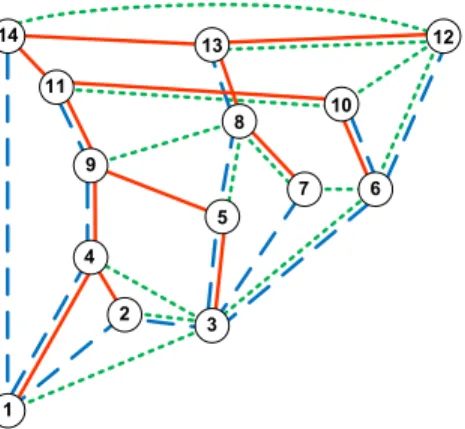
Let k spanning trees of a graph be independent if they all have the same root vertex r and, for

every vertex x 6 = r , the paths from x to r in the k spanning trees are internally disjoint (i.e.,

vertex-disjoint except for their endpoints; see Figure 5). The following conjecture from 1988 due

to Itai and Rodeh [21] has received considerable attention in graph theory throughout the past

decades.

Conjecture (Independent Spanning Tree Conjecture [21]) . Every k -connected graph contains k independent spanning trees.

14 11

1

2

12

9

3 8

10

7 6

4

5 13

Figure 5: Three independent spanning trees in the graph of Figure 1, which were computed from its Mondshein sequence (vertex numbers depict a consistent tr -numbering).

The conjecture has been proven for k ≤ 2 [21], k = 3 [6, 41] and k = 4 [8], with running times O(m), O(n

) and O(n

), respectively, for computing the corresponding independent spanning trees.

For every k ≥ 5, the conjecture is open. For planar graphs, the conjecture has been proven by Huck [19].

We show how to compute three independent spanning trees in linear time, using an idea of [6].

This improves the previous best quadratic running time. It may seem tempting to compute the spanning trees directly and without using a Mondshein sequence, e.g. by local replacements in an induction over BG-operations or inverse contractions. However, without additional restrictions this is bound to fail, as shown in Figure 6.

v

r

y z

x

Figure 6: A 3-connected graph G (some edges are not drawn). G is obtained from the 3-connected graph G

:= (G − v) ∪ xy by performing a BG-operation (or inverse contraction) that adds the vertex v (with added edge vy ). Two of the three independent spanning trees of G

are given, rooted at r (thick edges). However, not both of them can be extended to v .

Compute a Mondshein sequence through rt and avoiding u , as described in Theorem 17. Choose r as the common root vertex of the three spanning trees and let x 6 = r be an arbitrary vertex.

First, we show how to obtain two internally disjoint paths from x to r that are both contained

in the subgraph G

. A tr-numbering < is a total order v

< · · · < v

of the vertices of a graph

such that t = v

, r = v

, and every other vertex has both a higher-numbered and a lower-numbered

neighbor. Let a tr -numbering < be consistent [6] to a Mondshein sequence if < is a tr -numbering

for every graph G

, 0 ≤ i ≤ m − n . We can compute a consistent tr -numbering < in linear time as follows: Let <

be the total order on V ( P

) from t to r ; then <

is a consistent tr -numbering of G

. We maintain <

in the order data structure of [4] (see the computational complexity paragraph).

Now we add iteratively the next ear P

and obtain <

from <

by ordering the new inner vertices of P

from the lower to the larger endpoint of P

in <

(such that inner ( P

) is between these endpoints in <

). This takes amortized time proportional to the length of P

and, hence, gives a total linear running time.

According to < , every vertex x 6 = r has a higher-numbered neighbor in G

and every vertex x / ∈ {r, t} a lower-numbered neighbor in G

. Fixing arbitrary such neighbors, the first two spanning trees T

and T

then consist of the incident edges to higher neighbors and of the edge tr and the incident edges to lower neighbors, respectively. Clearly, T

and T

are independent due to the numbering used.

We construct the third independent spanning tree T

. As a Mondshein sequence is non- separating, every vertex x 6 = {r, u} has an incident edge with an endpoint in G

(as seen before, iterating this argument gives a path to u in G

). Let T

consist of arbitrary such in- cident edges and of the edge ru . Since G

and G

are vertex-disjoint, T

is independent from T

and T

.

Remark. We remark that the three independent spanning trees constructed this way satisfy the following additional condition: Due to the fact that T

and T

are extended to r by one single edge, all incident edges of r are contained in at most one of T

, T

, T

. In particular, no edge of G is contained in all three independent trees, which is a fact that cannot be derived from the definition of independent spanning trees (an edge that is incident to r may be contained in all three trees).

Application 2: Output-Sensitive Reporting of Disjoint Paths

Given two vertices x and y of an arbitrary graph, a k-path query reports k internally disjoint paths between x and y or outputs that these do not exist. Di Battista, Tamassia and Vismara [11] give data structures that answer k -path queries for k ≤ 3. A key feature of these data structures is that every k -path query has an output-sensitive running time, i.e., a running time of O ( ` ) if the total length of the reported paths is ` (and running time O (1) if the paths do not exist). The preprocessing time of these data structures is O ( m ) for k ≤ 2, but O ( n

) for k = 3.

For k = 3, Di Battista et al. show how the input graph can be restricted to be 3-connected using a standard decomposition. For every 3-connected graph we can compute a Mondshein sequence, which allows us to compute three independent spanning trees T

– T

in a linear preprocessing time, as shown in Application 1. If x or y is the root r of T

– T

, this gives a straight-forward output- sensitive data structure that answers 3-path queries: we just store T

– T

and extract one path from each tree per query.

In order to extend these queries to k -path queries between arbitrary vertices x and y , [11] gives a case distinction that shows that the desired paths can be found efficiently in the union of the six paths in T

– T

that join either x with r or y with r . This case distinction can be used for the desired output-sensitive reporting in time O ( ` ) without changing the preprocessing. We conclude that the preprocessing time of O(n

) for allowing k-path queries with k ≤ 3 in arbitrary graphs can be improved to O ( n + m ).

Application 3: Planarity Testing

We give a conceptually very simple planarity test based on Mondshein’s sequence for any 3-

connected graph G in time O ( n ). The 3-connectivity requirement is not crucial, as the planarity of

G can be reduced to the planarity of all 3-connected components of G , which in turn are computed

as a side-product from the computation of the BG-sequence [28, Appendix 2]. Alternatively, one could also use standard algorithms [18, 16] for reducing G to be 3-connected.

If m > 3 n − 6, G is not planar due to Euler’s formula and we reject the instance, so let m ≤ 3 n − 6. Let rt be an edge of G . We will find an embedding whose outer face is left of rt , unless G is non-planar. Due to Whitney [39], this embedding is unique. In light of Observation 11, we need to pick an edge ru 6 = rt such that tr ∪ ru is in a non-separating cycle. We can easily find such an edge by computing a Mondshein sequence through rt and avoiding some vertex u

∈ {r, t} / , and then taking the edge that is incident to r in P

− rt (alternatively, any linear-time algorithm that computes a non-separating cycle containing rt like the one in [6] can be used).

Now we compute a Mondshein sequence D through rt and avoiding u that satisfies Property 7.7 in time O ( n ). If G is planar, Observation 11 ensures that D is a canonical ordering of our fixed embedding; in particular, the last vertex u and the edge rt will be embedded in the outer face.

Due to Property 7.7, P

has no chords and every short ear xy satisfies birth ( x ) 6 = birth ( y ). For the embedding process, we rearrange the order of short ears in D such that all short ears xy with birth(x) < birth(y) are direct successors of the long ear P

(this can be done in linear time using bucket sort).

We start with a planar embedding M

of P

. Step by step, we attempt to augment M

with the next long ear P

in D as well as all short ears directly succeeding P

in order to construct a planar embedding M

of G

.

Once the current embedding M

contains u , we have added all edges of G and are done. Oth- erwise, u is contained in G

, according to Definition 6.2. Then G

contains a path from each inner vertex of P

to u , according to Lemma 5. Since u is contained in the outer face of the unique embedding of G , adding the long ear P

to M

can preserve planarity only when it is embedded into the outer face f of M

. Thus, we only have to check that both endpoints of P

are contained in f (this is easy to test by maintaining the vertices of the outer face). For the same reason, the short ears directly succeeding P

can preserve planarity only if the set S of their endpoints in G

is contained in f . Note that, if there is at least one such short ear, P

has precisely one inner vertex v due to Property 7.7 and all short ears directly succeeding P

have v as endpoint.

Thus, if the endpoints of P

and S are contained in f , we embed P

and the short ears into f in the only possible way, i.e. as a path or as one new vertex v with the short ears and the two edges of P

as incident edges. Otherwise, we output “not planar”. If desired, a Kuratowski-subdivision can then be easily extracted in time O ( n ), as shown in [32, Lemma 5] (the extraction is even simpler, as we do not make use of adding “claws”).

Application 4: Contractible Subgraphs in 3-Connected Graphs

A connected subgraph H of a 3-connected graph G is called contractible if contracting H to a single vertex generates a 3-connected graph. It is easy to show that a connected subgraph H is contractible if and only if G− V (H) is 2-connected. While many structural results about contractible subgraphs are known in graph theory, we are not aware of any non-trivial result that computes them.

Using a Mondshein sequence, we can identify a nested family of m − n contractible induced subgraphs in linear time, namely the subgraphs G

for every 0 ≤ i < m − n. Clearly, these subgraphs are contractible, as G − G

is 2-connected due to Lemma 7.5. Moreover, for each i > 0, G

is an induced subgraph of the induced subgraph G

. In particular, every G

contains u , since V

= {u} due to Definition 9.2.

Application 5: The k-Partitioning Problem

Given vertices a

, . . . , a

of a graph G and natural numbers n

, . . . , n

with n

+ · · · + n

= n , we