Testing for change in stochastic volatility with long range dependence

SFB 823

Testing for change in

stochastic volatility with long range dependence

Discussion Paper

Nr. 66/2016

Testing for change in stochastic volatility with long range dependence

Annika Betken ^∗ Rafa l Kulik^† November 6, 2016

Abstract

In this paper we consider a change point problem for long memory stochastic volatility models. We show that the limiting behavior for the CUSUM test statistics may not be affected by long memory, unlike the Wilcoxon test statistic which is influenced by long range dependence. We compare our results to subordinated long memory Gaussian processes. Theoretical properties are accompanied by simulation studies.

1 Introduction

One of the most often observed phenomena in financial data is the fact that the log- returns of stock-market prices appear to be uncorrelated, whereas the absolute log-returns or squared log-returns tend to be correlated or even exhibit long-range dependence. An- other characteristic of financial time series is the existence of heavy tails in the sense that the marginal tail distribution behaves like a regularly varying function. Both of these fea- tures of empirical data can be covered by the so-called long memory stochastic volatility model (LMSV, in short), with its original version introduced in [7]. For this we assume that the data generating process {Xj, j ≥1} satisfies

Xj =σ(Yj)εj, j ≥1, (1)

where

• {ε_j, j ≥1} is an i.i.d. sequence with mean zero;

• {Y_j, j ≥1} is a stationary, long-range dependent Gaussian process;

∗Ruhr-Universit¨at Bochum, Fakult¨at f¨ur Mathematik, annika.betken@rub.de; Research supported by the German National Academic Foundation and Collaborative Research Center SFB 823Statistical mod- elling of nonlinear dynamic processes.

†University of Ottawa, Department of Mathematics and Statistics, rkulik@uottawa.ca

• σ(·) is a non-negative measurable function, not equal to 0.

Note that within this model long memory results from the subordinated Gaussian sequence {Y_j, j ≥1}only. More precisely, we assume that {Y_j, j ≥1}admits a linear representation with respect to an i.i.d. Gaussian sequence {η_j, j ≥1} with E(η₁) = 0, Var(η₁) = 1, i.e.

Y_j =

∞

X

k=1

c_kη_j−k , j ≥0, (2)

with P∞

k=1c²_k = 1 and

γY(k) = Cov(Yj, Yj+k) =k^−DLγ(k),

where D∈(0,1) and L_γ is slowly varying at infinity. Also, we assume that

• {(ε_j, η_j), j ≥1} is a sequence of i.i.d. vectors.

The above set of assumptions we will call collectively LMSV model.

The tail behavior of the sequence {X_j, j ≥1}can be related to the tail behavior of ε_j orσ(Y_j) or both. Here we will specifically assume that

• random variables ε_j have a marginal distribution with regularly varying right tail, i.e. ¯Fε(x) :=P(ε1 > x) =x^−αL(x) for some α >0 and a slowly varying function L, such that the following tail balance condition holds:

x→∞lim

P(ε1 > x)

P(|ε₁|> x) =p= 1− lim

x→∞

P(ε1 <−x) P(|ε₁|> x) for some p∈(0,1];

• it holds

E

σ^α+δ(Y0)

<∞ for some δ >0.

Under these conditions, it follows by Breiman’s Lemma (see [17, Proposition 7.5]) that P(X₁ > x)∼E[σ^α(Y₁)]P(ε₁ > x), (3) i.e. the process {X_j, j ≥1}inherits the tail behavior from {ε_j, j ≥1}.

We would like to point out here that in the literature the usage of the term LMSV often presupposes that the sequences {Y_j, j ≥1} and {ε_j, j ≥1} are independent. In this paper we will consider a more general model: instead of claiming mutual independence of {Y_j, j ≥ 1} and {ε_j, j ≥ 1}, we only assume that (η_j, ε_j) is a sequence of independent random vectors. Especially, this implies that for a fixed index j the random variables ε_j and Yj are independent whileYj may depend on{εi, i < j}. In many cases this version of the LMSV model is referred to as LMSV with leverage.

1.1 Change-point detection under long memory

One of the problems related to financial data is to detect change points in the behavior of the sequence {X_j, j ≥ 1}. Although the problem has been extensively studied for independent random variables (see an excellent book [8]) or in case of weakly dependent data, the issue has not been fully resolved for time series with long memory. The researchers focused rather on justifying whether the observed long range dependence is real or is due to changes in weakly dependent sequences (so-called spurious long memory). See e.g. [3]

and Section 7.9.1 of [2] for further references on the latter issue.

As for the testing changes in long memory sequences, one of the first paper seems to be [13], where the authors showed that long range dependence affects the asymptotic behavior of the CUSUM statistics for changes in the mean. For the general testing problem with a change in the marginal distribution under the alternative hypothesis, [12] consider Kol- mogorov - Smirnov type change-point tests and change-point estimators for long memory moving average processes. Under the assumption of converging change-point alternatives in LRD time series, the asymptotic behavior of Kolmogorov-Smirnov and Cram´er-von Mises type test statistics has also been investigated by [22]. Likewise, [9] show that the Wilcoxon test is always affected by long memory. In fact, in the case of Gaussian long memory data, the asymptotic relative efficiency of the Wilcoxon test and the CUSUM test is 1.

In case of long range dependence, the normalization and the limiting distribution of test statistics typically depend on unknown multiplicative factors or parameters related to the dependence structure of the data generating processes. To bypass estimation of these quantities, the concept of self-normalization has recently been applied to several testing procedures in change-point analysis: In [19] the authors define a self-normalized Kolmogorov-Smirnov test statistic that serves to identify changes in the mean of short range dependent time series. [18] adopted the same approach to define an alternative normalization for the CUSUM test; [4] considers a self-normalized version of the Wilcoxon change-point test proposed by [9].

We refer also to Section 7.9 of [2] for further results on change-point detection for long memory processes.

1.2 Change-point detection for LMSV

In this paper we study CUSUM and Wilcoxon tests for LMSV model and discuss particular cases of testing changes in the mean, in the variance and in the tail index. Of course, the variance and the tail index can be regarded as the mean of transformed random variables, but we observe different effects for each of the three quantities. In particular, the main findings of our paper are as follows:

A-1: CUSUM tests for change in the mean for the LMSV models is typically not affected by long memory (see Corollary 3.2 and Example 4.1). This is different than the findings in [13] for subordinated Gaussian processes;

A-2: Wilcoxon test for change in the mean for the LMSV models is typically affected by long memory (see again Corollary 3.2 and Example 4.1). This is in line with the findings for subordinated Gaussian processes

Hence, to test changes in the mean for the LMSV it is beneficial to use CUSUM test.

B: CUSUM and Wilcoxon tests for change in the variance for the LMSV models are typically affected by long memory; see Section4.2.

B: CUSUM and Wilcoxon tests for change in the tail index for the LMSV models are typically affected by long memory; see Section4.3

The paper is structured as follows. In Section 2 we collect some results on subordinated Gaussian processes. In Section 3 we discuss the change-point problem. In particular, we consider CUSUM test and Wilcoxon test. The former is a direct consequence of the existing results, while the latter requires a new theorem on the limiting behavior of empirical processes based on LMSV data. Section4is devoted to examples in case of testing changes in the mean, in the variance and in the tail. Since the test statistics and/or limiting distributions involve unknown quantities, self-normalization is considered in Section 5.

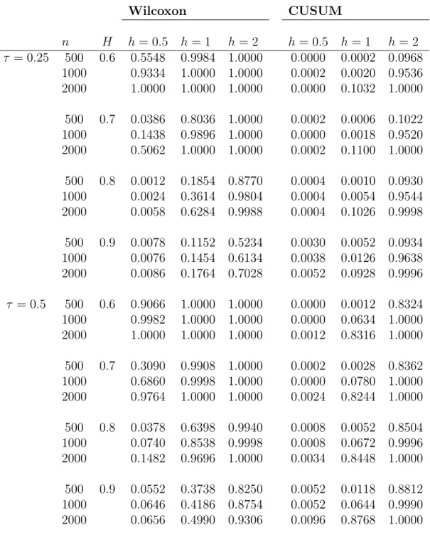
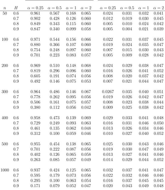
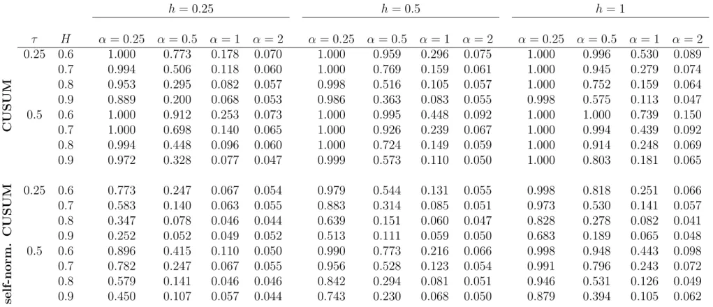
In fact, in Section 6 we perform simulation studies and indicate that self-normalization provides robustness.

2 Preliminaries

2.1 Some properties of subordinated Gaussian sequences

The main tool for studying the asymptotic behavior of subordinated Gaussian sequences is the Hermite expansion. For a stationary, long-range dependent Gaussian process {Y_j, j ≥ 1} and a measurable function g such that E(g²(Y₁)) < ∞ the corresponding Hermite expansion is defined by

g(Y₁)−E (g(Y₁)) =

∞

X

q=m

J_q(g)

q! H_q(Y₁), where H_q is the q-th Hermite polynomial,

Jq(g) = E (g(Y1)Hq(Y1)) and

m = inf{q≥1|J_q(g)6= 0} .

The integer m is called the Hermite rank of g and we refer to J_q(g) as the q-th Hermite coefficient of g.

We will also consider the Hermite expansion of the function class 1{g(Y₁)≤x}−F_g(Y1)(x), x∈R ,

where F_g(Y1) denotes the distribution function of g(Y₁). For fixedx we have 1{g(Y1)≤x}−F_g(Y1)(x) =

∞

X

q=m

J_q(g;x)

q! Hq(Y1) with

J_q(g;x) = E 1{g(Y₁)≤x}H_q(Y₁) .

The Hermite rank corresponding to this function class is defined by m= inf_xm(x), where m(x) denotes the Hermite rank of 1_{g(Y1)≤x}−F_g(Y1)(x). See [2].

The asymptotic behavior of partial sums of subordinated Gaussian sequences is char- acterized in [21]. Due to the functional non-central limit theorem in that paper,

1 d_n,m

bntc

X

j=1

g(Y_j)⇒ J_m(g)

m! Z_m(t), 0≤t≤1, (4)

where

d²_n,m = Var

n

X

j=1

H_m(Y_j)

!

∼c_mn^2−mDL^m(n), c_m = 2m!

(1−Dm)(2−Dm),

Z_m(t), 0≤t ≤1, is an m-th order Hermite process and the convergence holds inD([0,1]), the space of functions that are right continuous with left limits. In fact the limiting behavior in (4) is the same as that of the corresponding partial sums based on {Hm(Yj), j ≥1}:

J_m(g) 1 d_n,m

bntc

X

j=1

H_m(Y_j)⇒ J_m(g)

m! Z_m(t), 0≤t≤1.

Moreover, the functional central limit theorem for the empirical processes was established in [10]. Specifically,

sup

−∞≤x≤∞

sup

0≤t≤1

d⁻¹_n,m







bntc G_bntc(x)−E G_bntc(x)

−J_m(g;x)

bntc

X

j=1

H_m(Y_j)







−→P 0, (5) where

G_l(x) = 1 l

l

X

j=1

1_{g(Yj)≤x}

is the empirical distribution function of the sequence {g(Y_j), j ≥ 1} and −→^P denotes convergence in probability. Thus, the empirical process

d⁻¹_n,mbntc

Gbntc(x)−E Gbntc(x) , x∈(−∞,∞), t∈[0,1], converges in D([−∞,∞]×[0,1]) to Jm(g;x)Zm(t).

We refer the reader to [10], [21] and [2] for more details.

3 Change-point problem

Given the observations X₁, . . . , X_n and a function ψ, we define ξ_j =ψ(X_j), j = 1, . . . , n, and we consider the testing problem:

H₀ : E(ξ₁) =· · ·= E(ξ_n),

H1 :∃ k ∈ {1, . . . , n−1} such that E(ξ1) =· · ·= E(ξk)6= E(ξk+1) =· · ·= E(ξn). We choose ψ according to the specific change-point problem considered. Possible choices include:

• ψ(x) = x in order to detect changes in the mean of the observations X1, . . . , Xn

(change in location);

• ψ(x) =x² in order to detect changes in the variance of the observations X₁, . . . , X_n (change in volatility);

• ψ(x) = log(x²) or ψ(x) = log(|x|) in order to detect changes in the index α of heavy-tailed observations (change in the tail index).

It is obvious that ψ(x) = x and ψ(x) = x² lead to testing a change in the mean and variance, respectively. The choice ψ(x) = log(|x|) requires an additional comment. We note that (3) describes only the asymptotic tail behavior of X₁. For the purpose of this paper, we shall pretend that P (|X₁|> x) = c^αx^−α, x > c, for some c > 0. Then the maximum likelihood estimator of (1/α), the reciprocal of the tail index, is

1 n

n

X

j=1

log (|X_j|/c) . (6)

This estimator is used in the CUSUM test statistic. To resolve the problem of change-point in the tail index in full generality, we need to employ a completely different technique, based on the so-called tail empirical processes (see [15]). This will be done in a subsequent paper.

In any case, the following test statistics may be applied in order to decide on the change-point problem (H₀, H₁):

• The CUSUM test rejects the hypothesis for large values of the test statistic C_n = sup

0≤λ≤1

C_n(λ), where

C_n(λ) =

bnλc

X

j=1

ψ(X_j)−bnλc n

n

X

j=1

ψ(X_j)

. (7)

• The Wilcoxon test rejects the hypothesis for large values of the test statistic W_n = sup

0≤λ≤1

W_n(λ), where

W_n(λ) =

bnλc

X

i=1 n

X

j=bnλc+1

1{ψ(X_j)≤ψ(X_j)}− 1 2

. (8)

The goal of this paper is to obtain limiting distributions for the CUSUM and the Wilcoxon test statistic in case of time series that follow the LMSV model.

3.1 CUSUM Test for LMSV

In order to determine the asymptotic behavior of the CUSUM test statistic computed with respect to the observationsψ(X₁), . . . , ψ(X_n), we have to consider the partial sum process Pbntc

j=1(ψ(Xj)−E (ψ(Xj))).

For the observationsX₁, . . . , X_n that satisfy the LMSV model, the asymptotic behavior of the partial sum process is described by Theorem 4.10 in [2] and hence is stated without the proof. In order to formulate the result, we introduce the following notation:

F_j =σ(ε_j, εj−1, . . . , η_j, ηj−1, . . .),

i.e. F_j denotes theσ-field generated by the random variablesε_j, ε_j−1, . . . , η_j, η_j−1, . . .. Due to the construction ε_j is independent of Fj−1 and Y_j is Fj−1-measurable.

Theorem 3.1. Assume that {X_j, j ≥ 1} follows the LMSV model. Furthermore, assume that E(ψ²(X₁)) < ∞. Define the function Ψ by Ψ(y) = E (ψ(σ(y)ε₁)). Denote by m the Hermite rank of Ψ and by J_m(Ψ) the corresponding Hermite coefficient.

1. If E(ψ(X₁)| F₀)6= 0 and mD <1, then 1

dn,m bntc

X

j=1

(ψ(X_j)−E(ψ(X_j))) ⇒ J_m(Ψ)

m! Z_m(t), t∈[0,1], in D([0,1]).

2. If E(ψ(X1)| F0) = 0, then

√1 n

bntc

X

j=1

ψ(X_j)⇒σB(t), t∈[0,1],

in D([0,1]), where B denotes a Brownian motion process and σ² = E(ψ²(X1)).

As the immediate consequence of Theorem 3.1 we obtain the asymptotic distribution for the CUSUM statistic.

Corollary 3.2. Under the assumptions of Theorem 3.1, 1. If E(ψ(X₁)| F₀)6= 0 and mD <1, then

1 d_n,m sup

0≤λ≤1

C_n(λ)⇒ J_m(Ψ) m! sup

0≤t≤1

|Z_m(t)−tZ_m(1)| . (9) 2. If E(ψ(X₁)| F₀) = 0

√1 n sup

0≤λ≤1

C_n(λ)⇒√ σ sup

0≤t≤1

|B(t)−tB(1)| , where B denotes a Brownian motion process and σ² = E(ψ²(X₁)).

It is important to note that the Hermite rank of Ψ does not necessarily correspond to the Hermite rank of σ. See Section 4.

3.2 Wilcoxon test for LMSV

For subordinated Gaussian time series {g(Y_j), j ≥ 1}, where {Y_j, j ≥ 1} is a stationary Gaussian LRD process and g is a measurable function, the asymptotic distribution of the Wilcoxon test statistic W_n is derived from the limiting behavior of the two-parameter empirical process

bntc

X

j=1

1{g(Y_j)≤x}−F_g(Y1)(x)

, x∈(−∞,∞), t ∈[0,1], where F_g(Y1) denotes the distribution function of g(Y₁); see [9].

In order to determine the asymptotic distribution of the Wilcoxon test statistic for the LMSV model, we need to establish an analogous result for the stochastic volatility process {X_j, j ≥ 1}, i.e. our preliminary goal is to prove a limit theorem for the two-parameter empirical process

G_n(x, t) =

bntc

X

j=1

1{ψ(X_j)≤x}−F_ψ(X1)(x) ,

where now F_ψ(X1) denotes the distribution function of ψ(X1) with X1 =σ(Y1)ε1. To state the weak convergence, we introduce the following notation. Define

Ψ_x(y) = P(ψ(yε₁)≤x) .

Theorem 3.3. Assume that{X_j, j ≥1} follows the LMSV model. Moreover, assume that Z ∞

−∞

d

duP (ψ(uε1)≤x)du <∞. (10) IfmD <1, wherem denotes the Hermite rank of the class

1_{σ(Y1)≤x}−F_σ(Y1)(x), x∈R , 1

d_n,mG_n(x, t)⇒ J_m(Ψ_x◦σ)

m! Z_m(t), (11)

in D([−∞,∞]×[0,1]) .

The proof of this theorem is given in Section 3.3. At this moment we conclude the asymptotic distribution of the Wilcoxon statistics.

Corollary 3.4. Under the conditions of Theorem 3.3 1

nd_n,m sup

λ∈[0,1]

W_n(λ)⇒ Z

R

J_m(Ψ_x◦σ)dF_ψ(X1)(x)

1 m! sup

λ∈[0,1]

|Z_m(λ)−λZ_m(1)| . Proof of Corollary 3.4. According to [9], the asymptotic distribution of the Wilcoxon test statistic can be concluded directly from the limit of the two-parameter empirical process if the sequence {X_j, j ≥ 1} is ergodic. Ergodicity is obvious since X_j can be represented as a measurable function of the i.i.d. vectors {(η_j, εj), j ≥1}.

3.3 Proof of Theorem 3.3

To prove Theorem 3.3, we consider the following decomposition:

G_n(x, t)

=

bntc

X

j=1

1{ψ(X_j)≤x}−E 1{ψ(X_j)≤x}| Fj−1

+

bntc

X

j=1

E 1{ψ(X_j)≤x}| Fj−1

−F_ψ(X1)(x)

=:M_n(x, t) +R_n(x, t).

It will be shown thatn^−1/2M_n(x, t) =O_P(1) uniformly inx, t, whiled⁻¹_n,mR_n(x, t) converges in distribution to the limit process in formula (11). Theorem 3.3 then follows because

√n= o(d_n,m).

Martingale part. For fixedxthe following lemma characterizes the asymptotic behavior of the martingale part M_n(x, t). We write

M_n(t) :=M_n(x, t) =

bntc

X

j=1

ζ_j(x) with ζ_j(x) = 1{ψ(X_j)≤x}−E 1{ψ(X_j)≤x}| Fj−1

.

Lemma 3.5. Under the conditions of Theorem 3.3 we have

√1

nM_n(t)⇒β(x)B(t), t∈[0,1],

in D([0,1]), where B denotes a Brownian motion process and β²(x) = E(ζ₁²(x)).

Proof. Define

ζ_nj =n⁻¹²ζ_j(x) =X_nj(x)−E(X_nj(x)| F_j−1)

with X_nj(x) = n⁻¹²1_{ψ(Xj)≤x}. In order to show convergence in D([0,1]), we apply the functional martingale central limit theorem as stated in Theorem 18.2 of [6]. Therefore, we have to show that

bntc

X

j=1

E ζ_nj² | Fj−1

⇒β(x)t for every t and that

n→∞lim

bntc

X

j=1

E ζ_nj² 1{|ζnj|≥}

= 0

for everyt and >0 (Lindeberg condition). In order to show that the Lindeberg condition holds, it suffices to show that

n→∞lim

bntc

X

j=1

E

X_nj² (x)1{^|Xnj(x)|≥2}

= 0 (12)

due to Lemma 3.3 in [11]. As the indicator function is bounded, the above summands vanish for sufficiently large n and hence (12) follows.

Furthermore, the random variable E ζ_j²(x)| Fj−1

can be considered as a measurable function of the random variableY_j and therefore as a function of εj−1, εj−2, . . .. As a result, E ζ_j²(x)| Fj−1

is an ergodic sequence and it follows by the ergodic theorem that 1

n

bntc

X

j=1

E ζ_j²(x)| Fj−1

= bntc n

1 bntc

bntc

X

j=1

E ζ_j²(x)| Fj−1

P

−→tE(ζ₁²(x)) for every t.

The next lemma establishes tightness of the two-parameter process.

Lemma 3.6. Under the conditions of Theorem 3.3 we have

√1

nM_n(x, t) = O_P(1) in D([−∞,∞]×[0,1]).

The (technical) proof of this lemma is postponed to Section 7.

Long memory part. Finally, we prove weak convergence of the long memory part R_n(x, t).

Lemma 3.7. Under the conditions of Theorem 3.3, 1

d_n,mRn(x, t)⇒ J_m(Ψ_x◦σ)

m! Zm(t), in D([−∞,∞]×[0,1]) .

Proof. Note that

E 1{ψ(X_j)≤x}| Fj−1

= E 1{ψ(σ(Y_j)εj)≤x}| Fj−1

= Ψ_x(σ(Y_j))

becauseYj isFj−1-measurable andεj is independent ofFj−1. Furthermore, E (Ψx(σ(Yj))) = F_ψ(X1)(x), the distribution function of ψ(X₁) =ψ(σ(Y₁)ε₁). Hence,

R_n(x, t) =

bntc

X

j=1

(Ψ_x(σ(Y_j))−F(x))

=bntc Z ∞

−∞

Ψ_x(u)d Gbntc−EGbntc

(u), where

G_l(u) = 1 l

l

X

j=1

1{σ(Y_j)≤u}

is the empirical distribution function of the sequence{σ(Y_j), j ≥1}. We have, d⁻¹_n,mR_n(x, t)

=d⁻¹_n,mbntc Z ∞

−∞

Ψ_x(u)d Gbntc−EGbntc

(u)

=− (Z ∞

−∞

d

duP (ψ(uε₁)≤x)d⁻¹_n,m





 bntc

Gbntc(u)−EGbntc(u)

−J_m(σ;u) m!

bntc

X

j=1

H_m(Y_j)





 du

)

−

(Z ∞

−∞

d

duP (ψ(uε₁)≤x)d⁻¹_n,mJ_m(σ;u) m!

bntc

X

j=1

H_m(Y_j)du )

=:I₁(x, t) +I₂(x, t), where m denotes the Hermite rank of the class

1{σ(Y₁)≤x}−F_σ(Y1)(x), x∈R and Jm(σ;y) = E 1{σ(Y1)≤y}Hm(Y1)

.

Using the reduction principle (5) withg =σ and the integrability condition (10), we con- clude that the first summand converges to 0 in probability, uniformly inx, t. Furthermore,

I₂(x, t) =− (Z ∞

−∞

d

duP (ψ(uε₁)≤x)d⁻¹_n,mJ_m(σ;u) m!

bntc

X

j=1

H_m(Y_j)du )

=−d⁻¹_n,m

bntc

X

j=1

H_m(Y_j) (Z ∞

−∞

d

duP(ψ(uε₁)≤x)Jm(σ;u) m! du

) .

We have

d⁻¹_n,m

bntc

X

j=1

H_m(Y_j)⇒Z_m(t).

Moreover, integration by parts yields Z ∞

−∞

d

duP (ψ(uε₁)≤x)J_m(σ;u)du

= Z ∞

−∞

d

duP(ψ(uε₁)≤x) Z

1{σ(z)≤u}H_m(z)ϕ(z)dzdu

= Z ∞

−∞

H_m(z)ϕ(z) Z d

duP (ψ(uε₁)≤x) 1_{σ(z)≤u}dudz

= Z ∞

−∞

H_m(z)ϕ(z) Z ∞

σ(z)

d

duP(ψ(uε₁)≤x)dudz

= lim

u→∞P (ψ(uε₁)≤x) Z ∞

−∞

H_m(z)ϕ(z)dz− Z ∞

−∞

P(ψ(σ(z)ε₁)≤x)H_m(z)ϕ(z)dz

=−J_m(Ψ_x◦σ).

4 Examples

4.1 Change in the mean

To test a change in the mean we choose ψ(x) =x.

CUSUM:Recall that the function Ψ in Theorem 3.1 is defined as Ψ(y) = E (ψ(σ(y)ε₁)).

In this case

E(ψ(X₁)| F₀) = σ(Y₁) E(ε₁) = 0.

Therefore, the CUSUM statistic converges to a Brownian bridge. Hence,

• Long memory does not influence the asymptotic behavior of the CUSUM statistic for testing change in the mean.

Wilcoxon: Recall that Ψ_x(y) = P(ψ(yε₁)≤x). Using the integration by parts and noting that (d/dz)ϕ(z) =−zϕ(z) we have

J₁(Ψ_x◦σ) = Z ∞

−∞

P (ψ(σ(z)ε₁)≤x)zϕ(z)dz

= Z ∞

−∞

d

dzP (ψ(σ(z)ε₁)≤x)ϕ(z)dz = Z ∞

−∞

d dzP

ε₁ ≤ x σ(z)

ϕ(z)dz

= Z ∞

−∞

1 σ(z)

0

f_ε x

σ(z)

ϕ(z)dz ,

wheref_εis the density ofε₁(if it exists). Here, different scenarios are possible. Ifσ(y) =y² then z →

1 σ(z)

f_ε(x/σ(z))⁰ϕ(z) is antisymmetric for any x and any choice of f_ε. Hence, J₁(Ψ_x◦σ) = 0 and one can calculate that the Hermite rank of Ψ_x◦σ is 2. Ifσ(y) = exp(y) and e.g. ε1 is Pareto-distributed, i.e. for some α >0, c >0

f_ε(x) = (αc^α

x^α+1, x≥c 0, x < c ,. then, as a result,

Z ∞

−∞

e^−z αc^α x

exp(z)

α+11{exp(z)^x ≥c}ϕ(z)dz

=αc^αx^−(α+1) Z ∞

−∞

exp(zα)1{^log(^x_c)^≥z}ϕ(z)dz

=αc^αx^−(α+1) 1

√2π

Z log(^xc)

−∞

exp(zα− 1 2z²)

| {z }

>0

dz .

Hence, J₁(Ψ_x◦σ)6= 0. In any case,

• Long memory influences the asymptotic behavior of the Wilcoxon statistic, unlike the CUSUM one.

4.2 Change in the variance

To test a change in the variance we choose ψ(x) =x².

CUSUM:Recall again that the function Ψ in Theorem3.1is defined as Ψ(y) = E (ψ(σ(y)ε₁)).

Then

E(ψ(X₁)| F₀) =σ²(Y₁) E(ε²₁)6= 0

and hence long memory affects the limiting behavior of the CUSUM statistic. Moreover, J_m(Ψ) = E(ε²₁)

Z

σ²(z)H_m(z)ϕ(z)dz = E ε²₁

J_m(σ²),

i.e. the Hermite rank of Ψ equals the Hermite rank of σ². If mD < 1 then the limiting behavior of the CUSUM statistic is described by (9). Hence,

• Long memory influences the asymptotic behavior of the CUSUM statistic for testing change in the variance.

Wilcoxon: Recall again that Ψ_x(y) = P(ψ(yε₁)≤x). We have J₁(Ψ_x◦σ) =

Z ∞

−∞

P(ψ(σ(z)ε₁)≤x)zϕ(z)dz

= Z ∞

−∞

d

dzP(ψ(σ(z)ε1)≤x)ϕ(z)dz = Z ∞

−∞

d dzP

ε²₁ ≤ x σ²(z)

ϕ(z)dz

= Z ∞

−∞

1 σ²(z)

0

f_ε x

σ²(z)

ϕ(z)dz .

If σ(y) = exp(−y) then we are in the same situation as in case of testing the mean and hence J₁(Ψ_x◦σ)6= 0. Hence,

• Long memory influences the asymptotic behavior of the Wilcoxon statistic for testing change in the variance.

4.3 Change in the tail index

To test a change in the tail index we choose ψ(x) = log(x²).

CUSUM:In this case

E(ψ(X₁)| F₀) = log(σ²(Y₁)) + E(log(ε²₁))6= 0

and hence long memory affects the limiting distribution of the CUSUM statistic. Moreover, Jm(Ψ) = 2

Z

log(σ(z))Hm(z)ϕ(z)dz = 2Jm(log◦σ), so that the Hermite rank of Ψ equals the Hermite-rank ofh= log◦σ.

We note further that in case of ψ(x) = log(x²) we have 1

d_n,m

bnλc

X

j=1

log X_j²

−E log X_j²

= 2

d_n,m

bnλc

X

j=1

(logσ(Y_j)−E logσ(Y_j)) +

√n d_n,m

√1 n

bnλc

X

j=1

log ε²_j

−E log ε²_j .