Eﬀects of noise correlations on the performance of quantum error-correcting and -avoiding methods

(1)

Effects of noise correlations on the performance of quantum error-correcting

and -avoiding methods

I n a u g u r a l - D i s s e r t a t i o n zur

Erlangung des Doktorgrades

der Mathematisch-Naturwissenschaftlichen Fakult¨ at der Universit¨ at zu K¨ oln

vorgelegt von Stefan Borghoff

aus K¨ oln

Hundt Druck GmbH, K¨ oln

2009

(2)

Berichterstatter Dr. Rochus Klesse Prof. Dr. Claus Kiefer Tag der m¨undlichen Pr¨ufung 2009-06-22

(3)

Motivation

Once upon a time there was a land of eternal entanglement. Strange qubits lived in that land trying to protect their land of information. But there was a large enemy of them, named decoherence - destroying entanglements and with that the peaceful harmony of the unitary quantum computer. Then this work appeared showing a way out of this misery protected by decoherence-free subspaces and armed with quantum error correcting codes.

So the qubits were freed. And if they don’t decohere, they are still entangled.

(4)

(5)

Abstract

In the scope of this work the coherence of quantum information, which is encoded into a qubit register, is analysed. The qubit register is modelled by a spin chain with finite inter-spin distance. In most physically relevant realisations this spin chain irreversibly interacts with a surrounding environment, such that a spin-boson model is used to describe the setting. Due to the interaction decoherence occurs among the qubits register and quantum information gets lost. Mechanisms to slow down this decoherence process are investigated. For that purpose, the techniques of encoding qubits into decoherence- reduced subspaces and quantum error correction are used. In both cases only a linear subspace of the complete available Hilbert space of the spin chain is used as quantum code. The stability of such a code against decoherence has to be evaluated. This evaluation is performed on average over all states within the code by a code fidelity.

Zusammenfassung

Die Kohärenz von quantenmechanischer Information, gespeichert in einem Qubit- Register, wird analysiert. Dieses Register besteht aus einer Spinkette mit endlichem Ab- stand zwischen den Spins. Zur realistischeren Modellierung wird eine irreversible Wech- selwirkung mit einem umgebenden Wärmebad angenommen und das kombinierte System durch ein Spin-Boson-Model beschrieben. Die Wechselwirkung verursacht Dekohärenz, die zu einem Verschwinden der gespeicherten Information führt. Es werden Methoden zur Verlangsamung oder Unterbindung von Dekohärenz untersucht. Dazu zählen sowohl die Codierung in dekohärenzfreie Unterräume, als auch Quantenfehlerkorrektur. In bei- den Fällen wird Information in einem Unterraum des zur Spinkette gehörigen Hilber- traums codiert. Die Güte dieser Codes im Schutz vor Dekohärenz wird bewertet. Als Maß dient eine über alle Zustände des Codes gemittelte Fidelity.

(6)

(7)

Introduction

During the last decades quantum information theory became an important topic. One of the main subjects within this theory is the question how quantum information can be stored in the state of a corresponding quantum mechanical system. This system is used as quantum memory and a good knowledge about it is needed e.g. to run a quantum computer. In the early 80th the fundamentals for such a quantum computer were developed. This development started with Benioff [Ben80] who recognised that a classical Turing machine could be realised by a quantum mechanical system. Thereby, the quantum mechanical system is a quantum computer which is able to perform the tasks of the conventional Turing machine. Later on, it was observed that a quantum computer provides much more possibilities than only to emulate classical Turing ma- chines. For instance, Feynman [Fey82, Fey86] pointed out that the time evolution of solid state devices could be simulated by a quantum computer in a very efficient way.

Then, Deutsch [Deu85] developed the concept of a quantum Turing machine and pointed out its potentiality for faster computations due to quantum parallelism. By taking advantage of this parallelism, the time needed to factorise integers into primes decreases dramatically according to the famous Shor algorithm [Sho94]. Moreover, fast quantum search algorithms could be implemented as it was pointed out by Grover [Gro96].

The advantage of a quantum-bit (qubit) register in comparison to a conventional register relies on the fact that it can be in the superposition of a very large number of classical computational states. Preserving coherence of such a highly superpositional and in general strongly entangled state [Unr94, Joz97] is a challenge for the realisation of a quantum computer which has to be solved. Commonly entanglement gets quickly destroyed in a qubit register which is coupled to a surrounding environment [GJK⁺96, Zur03]. This process is called decoherence. It unavoidably occurs in a qubit register due to the fact that qubits need to be controlled by external mechanisms, which is in contradiction to a shielding of information within the qubit register against external degrees of freedom. Accordingly, in most physical realisations there is an irreversible interaction between qubits and environment. In many situations due to this interaction the initial state of the qubit system evolves into a classical state. During this process the quantum information, which is stored within the qubit register, gets lost.

Hence, a mechanism has to be invented to maintain as much quantum information as possible. In this field error-correcting and decoherence-avoiding techniques were invented. The first error-correcting schemes were independently derived by Shor [Sho95, CS96] and Steane [Ste96]. They recover a qubit register after distortion by external noise. The existence of these schemes for quantum states has been crucial for the development on this field. The key idea rapidly evolved into a complete theory of quantum error-correcting codes and subsequently to the concept of fault-tolerant

(10)

quantum computation [KLZ98]. Independently of quantum error-correcting techniques decoherence-avoiding methods were developed by Palma et al. [PSE97] and enhanced by e.g. Zanardi and Rasetti [ZR97] and Lidar et al. [LCW98]. These mechanisms make use of possible symmetries in the interaction of, say, a quantum register and its surrounding environment. The idea is to encode quantum information into those register states that are protected by symmetry against the decohering interaction. Inasmuch as the symmetry is satisfied, these states span a decoherence-free subspace in the register’s Hilbert space. Physical realisations of this concept will have to rely almost necessarily on symmetries that hold only to some approximation. Encoding into subspaces that respect these symmetries can then provides partial protection against decoherence, to an extent that will depend on the actual realisation. In the scope of this work error- correcting and -avoiding methods as well as their combination are analysed. Thereby, a spin-boson model, which was already used by G. M. Palma et al., is used to describe a physical implementation. This model, which showed decoherence-free subspaces due to its symmetry, is transformed according to implementations with distant qubits into a model without symmetry. Then, the former decoherence-free subspaces are analysed.

Specifically, subspaces are considered that correspond to encoded quantum registers in which logical qubits are encoded in locally grouped spins. A measure to analyse such subspaces is also developed within this work. In comparison to older approaches on this topic here the correlations between qubits are analytically taken care of. Afterwards, quantum error-correction on the investigated model in combination with the investigated subspaces is considered.

The schedule of this work is presented in the following. An introduction to the phenomenon of decoherence is given in Chapter 1. As already outlined above, decoherence occurs in an open quantum system which is part of a larger closed system. Interactions between the investigated open quantum system and the remaining system lead to decoherence. As fundamental system of this work then-spin-boson model is analysed. This model is used in literature to describe a single or a couple of spins interacting with a surrounding bosonic environment [BP02]. The spin part of this model is used as qubit register. Accordingly, among the spins decoherence emerges due to interactions with the bosonic environment.

One of the spin-boson model’s most important features is that many physical realisations of qubit registers can be mapped onto it as an effective theory. To illuminate this mapping, different physical realisations of qubits are introduced exemplarily. For instance with atoms it is possible to construct spin qubits or qubits formed by the ground and an excited state. A typical candidate for the bosonic environment is given by thermal radiation. Other possibilities to construct qubits are given by Josephson junctions or quantum dots [BVJD98, LD98]. This list is by far not complete but gives an outlook of the basic idea to construct qubits and the mapping onto the spin-boson model.

Afterwards, the dynamics of the spin-boson model is analysed, as it effectively describes all these realisations. For that purpose, in Chapter 2 the time evolution of the n-spin-boson model is investigated. First the complete time evolution of the closed system is determined. Then its reduction to the spin system is calculated by tracing

(11)

out environmental degrees of freedom. The resulting time evolution of the spin system is interpreted as a quantum noise process. An analytical solution for this problem is presented for dissipationless couplings between spin part and environment. Within this work the cases of Ohmic and super-Ohmic spectral densities are outlined in full detail.

Finally, the noise of a dissipative model is dealt with in Chapter 6. In this case the time evolution is determined by a master equation of Bloch-Redfield type. Detailed knowledge about the decoherence of the considered qubit register is needed to deal with further questions concerning quantum memory.

Chapter 3 deals with the encoding of quantum information into quantum codes. In general, quantum codes are subspaces of the spin part’s Hilbert space. Having nspins, it is possible to encode a number ofk≤nlogical qubits within a subspace of the desired dimension. As different states of the spin system can be affected in different ways by their interaction to the environment some of them are superior to others. In particular, in the case of spins that are located at one point there are decoherence-free subspaces known which emerge due to symmetry. If the distance between the spins is finite the former symmetry is absent and consequently the codes cease to be decoherence-free.

This project deals with the question how these codes can be used in the case of finite inter-spin distance. Accordingly, special codes are presented which are used for further investigation. These codes are called symmetric codes. To decide whether a given code is a good candidate or not, a measure for codes is needed.

This is realised by the code fidelity presented in Chapter 4. By means of this fidelity it is possible to determine the robustness of a given quantum code against the disturbing effects of an acting noise. Starting point to derive the code measure is the channel fidelity. As the channel fidelity itself is only a measure between two quantum states, it is outlined how a useful measure for a complete code is constructed. In this context the average fidelity and entanglement fidelity of a quantum code are derived. The average fidelity is an averaged channel fidelity over all possible states of the code. Thereby, the channel fidelity of each state and its time evolved state is averaged. The entanglement fidelity is a lower bound for the average fidelity which converges to the average fidelity with increasing code size [HHH99, Nie02]. Both of them can be used as a code fidelity.

Afterwards, a connection of the entanglement fidelity to experiments is outlined. This connection grounds on the fact that for a dissipationless model the entanglement fidelity and a spin echo measurement [Ram49, Hah50] provide the same information. In case of a dissipative setting this is only approximately correct as long as timescales much lower than the relaxation time of the system are concerned.

Finally, in Chapter 5 the symmetric codes are evaluated using the entanglement fidelity as measure. First, the case of a dissipationless coupling is investigated. This result is compared to the evaluation of a plain qubit register without any encoding. It turns out that there exists a critical time beyond which an encoding into the symmetric codes is superior to plain qubits.

An even greater task than determining the fidelity of a given code is to find the optimal code. This problem is also discussed in Chapter 5. Unfortunately, it is not possible to give a solution to this problem in the scope of this work. Nevertheless, a

(12)

simplified problem can be formulated and dealt with. Thereby, the optimal encoding for a single qubit having a dissipationless coupling is determined. Instead of a spin chain, a generalised tetrahedron where all spins have equal distance to each other is analysed first. The optimisation process for this setting leads to the insight that symmetric codes provide the best encoding. In a generalised model of a spin chain this result is confirmed by a numerical method. So far, only dissipationless models were analysed. The missing dissipative couplings are examined in Chapter 6 with the help of the above mentioned master equation. Again, the encoding of a single qubit is investigated and the benefits of the previously introduced symmetric codes in comparison to plain qubits are pointed out.

Quantum error correction applied to the dissipationless model is considered in Chap- ter 7. In a first step the time evolution of the qubit register is transformed into a Kraus representation [KBDW83, NC00]. This form of noise seems to be best suited to calculate the quantities needed to evaluate quantum codes in combination with quantum error correction. Again, the entanglement fidelity is used as measure to evaluate the codes. In a first step symmetric codes without error correction are compared to locally optimised random codes with quantum error correction. As expected, randomly chosen codes perform better than symmetric codes, except for very weak couplings. In a second step quantum error correction is applied onto the symmetric codes. Surprisingly, it turns out that quantum error correction on randomly chosen codes is more effective than quantum error correction on symmetric codes.

(13)

1 The point of interest

In the 80th the idea to use quantum mechanical systems as quantum computers came up. Having such a quantum computer provides the possibilities to handle solid state problems [Fey82, Fey86], search algorithms [Gro96] and many other challenging tasks in a smart way. A main ingredient of each quantum computer is its quantum memory which is used to store quantum information within. Therefore, quantum memory is analysed in this work. Quantum memory consists of several quantum mechanical bits, called qubits.

Commonly, qubits occurring in quantum mechanical algorithms like the famous Shor algorithm [Sho94] for factorising integers are in general in highly superpositional and strongly entangled states. For the functionality of a quantum computer the coherence of these states has to be preserved. Accordingly, a good knowledge and control about each involved qubit is very important. To develop this knowledge, the construction of single qubits is focused on in this chapter. Then, having single qubits allows a generalisation to larger qubit registers. Thereby, qubits are not considered independently as they have a shared environment which establishes correlations between them. It turns out that there is a large zoo of possible candidates in nature to form single qubits. In the scope of this work some of the most common candidates are discussed. Namely, atomic spin qubits and qubits build by Josephson junctions [BVJD98] or quantum dots [LD98] are presented.

In each case the corresponding fundamental models are examined to outline the physical components of the qubit and its environment. Finally, to represent a qubit, two quantum mechanical states of the describing model have to be chosen. For each model these qubit states are manifested and the interaction to the corresponding environment is pointed out. In a next step an effective model is derived from the qubit states, the environment and the interaction between. To keep the examination as simple as possible in Sec. 1.3 each of the derived effective models is mapped onto a spin-boson model. Accordingly, only this model is discussed in full detail. An introduction to the spin-boson model is presented in Sec. 1.2. The spin part of this model forms the qubit register. A major problem for this qubit register is its sensitivity to the quantum noise occurring due to couplings to the environment. Here, the qubit register is a subsystem of the spin-boson model and accordingly interacts with the bosonic environment. Commonly, due to this interaction between environment and register decoherence might occur which makes it quite challenging to preserve the coherence of such a register. An introduction to decoherence is given in Sec. 1.1. The complete information about the decoherence of a specific system is included in its corresponding quantum noise. This noise is determined by the interaction Hamiltonian of the investigated case. Thereby, the occurring coupling coefficients in combination with the environment play a role.

(14)

CHAPTER 1. THE POINT OF INTEREST

1.1 Decoherence in an open quantum system

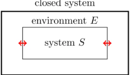
The study of decoherence was initiated in the 70th and 80th with the work on the emergence of classicality in the framework of quantum mechanics by Zeh [Zeh70] and Zurek [Zur81]. To get a feeling for decoherence, this section elaborates on the typical behaviour of a suitable systemSinteracting in an irreversible manner with a surrounding environmentE. An illustration of this setting is given in Fig. 1.1. In the scope of this work the system S is used as quantum memory and the environment is assumed to contain a large number of degrees of freedom. Although the environmental degrees of freedom are treated quantum mechanically, their state is taken unobservable for all practical purpose. The combined system ofS and E is considered as a closed quantum mechanical system, labelled SE. Any initial state ρ_SE(0) of this joint system evolves

closed system environmentE

systemS

Figure 1.1: The figure shows a schematic picture of the closed system SE with its constituentsS(system) andE(environment). Arrows symbolically represent an existing interaction between the two parts as explained above.

unitary in timet according to Schr¨odinger’s equation to a stateρSE(t). In a physically relevant setting for quantum information theory the initial state ρ_SE(0) is taken as a product state of system- and environment part. Thereby, the environment is assumed to start in thermal equilibrium whereas no restrictions are made to the system’s initial stateρ(0) as it corresponds to the actual quantum information. In contrast to the time evolution of the joint system, the time evolution of the reduced density operator of the systemS, which is obtained by tracing out all environmental degrees of freedom,

ρ(t) = tr

E{ρ_SE(t)}, (1.1)

is not unitary in general. Due to the fact that the stability of quantum information is concerned, this reduced density of the system S at time t has to be compared to its initial state. To illuminate the reduced system’s dynamics, the operator T_t : ρ(0) 7→ T_t(ρ(0)) ≡ ρ(t), mapping the reduced density operator ρ(0) on its time evolved density operatorρ(t), is investigated. It can be shown that the operatorT_tis of the form

T_t(ρ) =U_t◦ N_t(ρ), (1.2)

(15)

1.2. THE N-SPIN-BOSON MODEL whereU_t is a purely unitary operator, andN_tis a non-unitary completely positive map.

Various authors in [PSE97, DG98, BLW99, NC00, RQJ02, BP02] have established this form. Dealing withN_t, different behaviours occur depending on the present Hamiltonian.

Non trivial effects caused by N_t are topic of this work. For example, if the intrinsic energy of the eigenbasis of the systemS is preserved by the Hamiltonian, occurring non- trivial effects caused by the operator N_t are called decoherence if they lead to a loss of coherence. In this case the non-diagonal terms in the reduced density operator vanish. In general due to decoherence an entangled stateρ(0) continuously evolves into a classical state [GJK⁺96, Zur03]. For a non-energy preserving Hamiltonian also dissipative effects might occur and would also be contained in N_t. Here, an energy exchange with the environment leads to thermalisation of the initial state. Often such a dissipative setting is accompanied by decoherence. Concluding, the chosen form of the interaction between system and environment determines if decoherence and dissipation occurs.

1.2 The n-spin-boson model

For the purpose of this work, a special spin-boson model is used to represent a finite number of qubits coupled to an environment. As usual, the spin-boson model is a combined model, consisting of two parts. The first part of the model, labelled S, is a lattice of spin-¹/2 carrying objects. This lattice is considered to be one- or more- dimensional, having an equidistant inter-spin distanceaand a finite quantity ofnlattice sites. Each spin itself has the functionality of a single qubit. The second part of the model is a shared environment E which is a bosonic bath locally interacting with all spins. As no other external interactions are taken into account, the combined model of these two parts, labelled SE, is a closed system.

1.2.1 The Hamiltonian of the effective model

The full Hamiltonian, describing a lattice of spins coupled to an external bath, is divided into a free and an interacting part, ˆH = ˆH₀+ ˆH_I. Here, the free Hamiltonian ˆH₀must not contain terms that include any interaction between the spin system and the environment.

According to this condition the free Hamiltonian divides into a spin and an environment part,

Hˆ0= ˆHS+ ˆHE. (1.3)

The first term ˆHS describes the spin system. Its explicit form, introducing the energy splitting , reads

HˆS = 2

X

m

Zm⊗1E . (1.4)

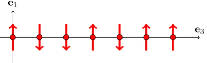
The index m is a tuple of positive integers with the dimension of the spin system and labels different lattice-sites. Z_m ≡ σ_z,m is a Pauli spin matrix acting on the spin on the lattice sitem. For simplification only the one-dimensional case of a spin chain with m ∈ N0e3 is investigated. According to this notation the spin-carriers are arranged along thee₃-axis. The energy splitting of each spin is taken to arise along thee₁-axis as

(16)

shown in Fig. 1.2. In the spin-boson model the spins are surrounded by an environment,

e3

e₁

Figure 1.2: The qubits are arranged in a chain along thee3-axis with equidistant inter- spin distance.

often called bath. This environment is modeled by bosonic excitations. The Hamiltonian of this bath, being the second term in Eq. (1.3), is given by

Hˆ_E =1S⊗X

k

~ω_kb^†_kb_k. (1.5)

This Hamiltonian consists of bosonic annihilation operatorsb_kand creation operatorsb^†_k. A set of these operators belongs to thek^thbath mode with energy ~ωk. Thermal radiation as a typical candidate would lead to a three-dimensional bath, but corresponding to a different setting also another dimension of the bath would be possible. The interaction Hamiltonian ˆHI of the spin-boson model describes the interplay between spin system and bath. ˆH_I is given in the form of

HˆI = cosηHˆZ+ sinηHˆX, (1.6) with a dimensionless control parameterη. The first term of the interaction Hamiltonian describes a dissipationless coupling via

Hˆ_Z =X

m

Z_m⊗B(am). (1.7)

Here,Zm is the Pauli spin matrix that already occurred in Eq. (1.4). The other term of the interaction Hamiltonian leads to a dissipative coupling by

Hˆ_X =X

m

X_m⊗B(am). (1.8)

The operator X_m is a Pauli spin matrix corresponding to the above mentionedZ_m. In both cases bosonic field operators

B(r) =X

k

g|k|e^−ik·rb^†_k+H.c. (1.9)

(17)

1.3. PHYSICAL REALISATIONS OF QUBITS with coupling coefficientsg|k|occur. Each of these coupling coefficients acquires a phase e^−ik·r, reflecting the wavelike character of the bosonic modes. Except for this phase the coupling is isotropic and identical for all spins. The coupling coefficients carry information about the spin-environment coupling and are specified in form of a spectral density

J(ω) =αω^se^−ω/Ω = 4X

k

δ(ω−ωk)|g_|k||², (1.10) with linear energy-momentum relation ωk =c|k|, high-energy cut-off Ω and the speed of the bosons c. The parameter s is called spectral parameter. This parameter has to respect the dimension of the bath. In case of a three-dimensional bathshas a two-times larger exponent as in comparison to an one-dimensional bath according to the Jacobi determinant of a coordinate transformation from Cartesian coordinates to spherical ones.

The coefficient α is ω-independent and can be read off in each |g_k|² by respecting the ω-independent part of the Jacobi determinant and an integration over occurring angles.

With this definition of a spectral density it is possible to replace the sum over discrete modes P

k|g_k|² by the integral R∞

0 dω J(ω) over a continuum.

This work mainly deals with two different regimes of the spectral density. One of them is the Ohmic setting having a spectral parametersbeing equal to one. The discussion of this case is of further interest as many dissipative models can effectively be described by a dissipationless model having an Ohmic coupling. This happens in particular if the bath acts one-dimensional. The other setting is e.g. needed to describe atomic absorption and emission processes and is given for a spectral parametersbeing equal to three. Dealing with other couplings requires the same tools as the are presented for the settings of s= 1,3.

1.3 Physical realisations of qubits

Starting from a microscopic view, this section elaborates on some physical realisations of qubits. Each of these realisations finally is given by an effective Hamiltonian. In the scope of this work only effective Hamiltonians which can be mapped onto a spin- boson model are observed. The first part, Sec. 1.3.1, deals with the usual matter- radiation interaction of atoms. Here, different physical implementations are considered.

For example, the model of an atomic spin coupled to a magnetic field is discussed.

Afterwards common photon absorption and emission processes are analysed, which will play a role, if qubits are constructed via different states of an atom. The rest of this section deals with Josephson junctions in Sec. 1.3.2 and quantum dots in Sec. 1.3.3.

There are two aims for the rest of this chapter. The first aim is to give insight to the fundamental models and a taste of the different mechanisms which are used to construct qubits. A concrete mapping for each of the presented systems on a spin-boson model is given in detail. The second aim of this section is to determine the spectral parameter s for different models as the behaviour of decoherence varies with s. This difference is further investigated in Chapter 2.

(18)

CHAPTER 1. THE POINT OF INTEREST 1.3.1 Atom-field interaction Hamiltonian

To describe the coupling of a single atom to an electromagnetic field, the minimal coupling Hamiltonian is investigated. Starting with this Hamiltonian the qubit states have to be selected. Possible candidates are given by the states of an atom’s electron of charge eand massm. In the given setting this electron interacts with an external electromagnetic field, given by a vector potential A and scalar potential Φ. Therefore, the model is described by the minimal coupling Hamiltonian which is given by

Hˆ = (ˆp−eA(r, t))²

2m +eΦ(r, t) +V(r)−µ_j·(∇ ×A(r, t)). (1.11) Here, the free Hamiltonian (without interaction to the electromagnetic field) of the electron itself is identified as

Hˆ_S = p²

2m +V(r). (1.12)

At this point the explicit structure of the qubit has to be chosen. In the following, two different possibilities are outlined. During the next part a spin qubit is presented. In this case the level splitting of the electron ground state due to a static magnetic field gives the two needed qubit states. Afterwards another possibility is presented. Thereby, the ground and first exited state of the electron in the absence of a magnetic field form the qubit.

Construction of a spin qubit. Calculations in the following paragraph are performed in hydrogen approximation. Accordingly, only the state of the outer electron of an atom is described by this method, such that this approximation is good for most alkali metals.

As mentioned above, the quantum-mechanical degree of freedom used for the qubit is the spin of the outer electron. This kind of qubit can be realised with cold Caesium atoms e.g., which is referred to in [GWO00, SDK⁺04]. In the scope of the cited work a dipole trap is used to arrange the atoms along the desired lattice, as shown in Fig. 1.2.

This arrangement is performed by a focused laser beam, such that the induced electric dipole moment together with the occurring dipole force keeps the atom in the centre of the trapping beam. Additionally, a static magnetic field causes the energy splitting of the spin systems Hamiltonian (cf. Eq. (1.4)) and keeps the magnetic axis of each atom fixed. To construct a qubit with full functionality it has to be possible to apply operations on them. In the present case all kind of needed operations can be performed by applying further external fields on the qubit lattice.

To continue, the interaction of the introduced spin qubit to an environment is pointed out. In the scope of this work an interaction due to the magnetic field of thermal radiation is investigated. The corresponding Hamiltonian is read off by the last term of the minimal coupling Hamiltonian in Eq. (1.11). Accordingly, the interaction Hamiltonian has Zeeman shape

Hˆ_I=−µ

j ·B, (1.13)

where B= ∇ ×A is the external magnetic field due to thermal radiation. The vector

(19)

1.3. PHYSICAL REALISATIONS OF QUBITS µ_j is connected to the total momentum operatorjof the electron. The total momentum operator is given by the sum of spin operator s and orbital momentum operator l as j=l+s. The related vector µ

j is given by

µ_j =µ_s+µ_l=−µ_B2s+l

~ . (1.14)

In the declared setting of an outer electron in an alkali metal, the orbit with l = 0 is occupied by the electron. Therefore, only the spin contributes to the interaction Hamiltonian. At this point the quantised version of the magnetic field is inserted into the Hamiltonian. For a derivation of the quantised magnetic field see e.g. the references [Lou73, SZ97]. To announce notation a short presentation of this derivation is delivered in Appendix C. There it becomes clear that the quantised magnetic field is optimal adapted to the problem if it is presented in the interaction picture. Following the presented instruction delivers the interaction Hamiltonian in the interaction picture,

H˜_I(t) =µ_BX

m

σ_m·1 c

√i ν

X

k,λ

r

~ω_k 20

a_kλe^i(kr^m^−ω^k^t) k

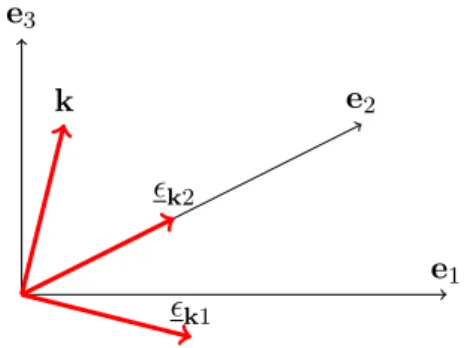
|k|×_kλ+H.c. (1.15) Here, σ is the vector of Pauli matrices and ν the quantisation volume. The vectors _kλ are polarisation vectors belonging to wave vectorkand polarisationsλ= 1,2, such that {k, ˆ _k1, _k2} forms an orthonormal basis. These polarisation vectors for a given wave vectork are illustrated in Fig. 1.3.

Following the concept that was presented at the beginning of this chapter, the spectral parameter s, which was introduced in Eq. (1.10), is determined. For that purpose, the coupling coefficients g_k have to be identified in the presented form of the interaction Hamiltonian in Eq. (1.15). Taking the absolute square of these coefficients and neglecting its ω-dependence produces the coupling coefficient α up to a dimensionless constant.

Here, this coupling constant of the spectral density is proportional to α∼µ²_B1

c² 1 (2π)³

~

2₀ = µ²_B

2π³c²~₀. (1.16)

The dimension of the bath enters into the calculation of the spectral parameter. A short analysis of the occurring|g_k|² shows that this expression growths linearly withω.

According to Eq. (1.10) the spectral parameter turns out to bes= 3.

Now some further illumination on the given interaction Hamiltonian is performed.

as it is illustrated in Fig. 1.2. In principle the interaction Hamiltonian in Eq. (1.15) contains couplings via all Pauli spin matrices due to σ. For simplification a restriction to the coupling via the Pauli spin matrixZ byZ⊗B_zis performed. The coupling in this case is dissipationless. It should be mentioned that the couplings via X and Y can be handled analogously. Just to remember, the homogeneous magnetic field, which leads to the Zeeman splitting of the spins, is applied alonge1-direction, Hence, thez-component of the magnetic field in the chosen basis isB_z =B·e₁. According to the derivation of

(20)

the magnetic field it is given as a sum over all photonic modes with wave vectorsk (cf.

Eq. (C.24) in Appendix C). At this point the continuum limit of these photonic modes is performed. Conveniently, spherical coordinates with radial distancek, azimuth angle ϕand zenith angle θare introduced. For a qubit, which is arranged along thee3-axis at

e1

e2

e₃ k

_k1 _k2

Figure 1.3: Picture, showing the vectorkand associated polarisation vectors for ϕ= 0 and θ=^(e3,k).

positionr, the projection of the magnetic field on the selectedz-direction is given by B_z(r) =X

k

g_|k| e₁·X

λ

kˆ×_kλa_kλ

!

e^i(k·r−ω^k^t)+H.c. (1.17)

=X

k,ϕk,θk

g_|k|(cosθ_kcosϕ_ka_k2−sinϕ_ka_k1)e^i(kr^cos^θ^k^−ω^k^t)+H.c. (1.18) The complex coupling constantsg_|k|can be read off e.g. in Eq. (1.15). The given form of the magnetic field is easy to verify using the proper polarisation vectors, having Fig. 1.3 in mind. By the selected choice of coordinates it turns out that only the length of r occurs in the equation, such thatB_z(r)≡B_z(r). Furthermore it can be established that for eachkthe expectation value of two of these magnetic fields at positions r_a and r_b is given by

D

Bz(ra)Bz^†(r_b) E

= |g_|k||²(cosθ_kcosϕ_k − sinϕ_k)e^ik|r^a^−r^b^|^cos^θ^k D

2a^†_ka_k+ 1 E

. Note that only the distance r between the two qubits at position r_a and r_b comes into play. An important class of functions consiting of this expectation value are the spectral correlations, which are used later on to describe the time evolution of qubits.

Anticipatory, the continuum limit of the bath modes is closer investigated. Occurring integrals have the form

I[f(k, ϕ, θ), r] =

∞

Z

0

dk

2π

Z

0

dϕ

π

Z

0

dθ k²sinθe^ikr^cos^θf(k, ϕ, θ), (1.19) wheref is a function depending on the two involved magnetic fields. In the present case

(21)

1.3. PHYSICAL REALISATIONS OF QUBITS f turns out to be f(k, ϕ, θ) = (cosθcosϕ − sinϕ)²D

2a^†_ka_k+ 1E

. To calculate the desired expectation value of B_z(r_a) and B_z(r_b) the following integrals are important:

I0[f(k), r] :=I[f(k), r] = 4π

∞

Z

0

dk k²sin (kr)

kr f(k), (1.20a)

I₁[f(k), r] :=I[f(k) sin²θ, r] = 8π

∞

Z

0

dk k²sin(kr)−krcos(kr)

k³r³ f(k) (1.20b) andI[f(k) cos²ϕcos²θ, r] =I0[f(k), r]/2−I1[f(k), r]/2. (1.20c) Obviously I[f(k) sin²ϕ, r] =I0[f(k), r]/2 holds. Finally the desired integral over expectation values of the magnetic fields is given by

Z

R³

dk D

B_z(r_a)B_z^†(r_b)E

=I₀h

f˜(k), ri

−I₁h

f˜(k), ri

/2 (1.21)

withr =|r_a−r_b|and ˜f(k) =|g_|k||²D

2a^†_ka_k+ 1 E

. In the following calculations the term I₁[|f(k), r]/2 is neglected for the sake of simplicity. In principle all methods that are˜ needed to handle this term are shown later on.

Qubit construction using the ground and first excited state. In this paragraph the minimal coupling Hamiltonian (cf. Eq. (1.11)) without Zeeman energy,

Hˆ = (ˆp−eA(r, t))²

2m +eΦ(r, t) +V(r), (1.22) is used, neglecting the spin of the electron. This setting is motivated in the absence of a static magnetic field. Here, an electron bound by a potential V(r) to a force centre located at r₀ is investigated. In the scope of this work the qubit’s two level system is determined by the ground state |gi ≡ |1i and the first exited state |ei ≡ |0i of the electron. To arrange the atomic lattice a magnetic trap might be used. This trap holds each atom due to its magnetic dipole momentum in position. A possible candidate for interactions is again given by thermal radiation. Accordingly the vector potentialA and scalar potential Φ of the thermal radiation determine the environment. The vector potential (cf. Eq. (C.22) in Appendix C) of a plane electromagnetic wave is given by A(r0+r, t) =P

kgk(t)e^ik·(r⁰^+r).This potential may be written in dipole approximation as

A(r₀+r, t) =X

k

g_k(t)e^ik·r⁰+O(k·r)

. (1.23)

A good justification for the dipole approximation is given if each wave only varies a little on the length of the atom. This is formally achieved for k·r1. Here, the high energy cutoff Ω introduced in Eq. (1.10) can be used to ensure this condition. A local

(22)

gauge transformation is applied on the minimal coupling Hamiltonian in Eq. (1.22). The gauge field for this transformation is given byχ(r, t) = −eA(r₀, t)·r.The corresponding transformation of the wavefunctionψ, vector potentialAand scalar potential Φ is given by

ψ7→ψe^iχ, A7→A+ 1

e∇χ and Φ7→Φ−1

e∂tχ . (1.24) After this gauge transformation the approximated minimal coupling Hamiltonian reads

Hˆ = p²

2m +eA(r˙ 0, t)·r+V(r). (1.25) Within this Hamiltonian the free part of the electron is identified to be ˆH_S = _2m^p² +V(r).

The remaining term provides the interaction Hamiltonian. The vector potential fulfils A˙ =−E, such that the interaction Hamiltonian in this setting is identified to be

Hˆ_I=−E(r₀, t)· D, (1.26)

whereD = er is the dipole operator.

Now the interaction Hamiltonian for a concrete setting is investigated. Again the question for the spectral parameter s (cf. Eq. (1.10)) arises. Further progress is achieved under some assumptions. A single atom at position r0 is investigated. For simplification the dipole momentum of the atom is assumed to point in Cartesian e₁ direction. In this case the scalar product between electric field and dipole is E · D = |E(r₀, t)|(cosθcosϕ − sinϕ)℘eg, as e1·P

λ_kλ = cosθcosϕ−sinϕ. The occurring scalar dipole momentum ℘eg is defined as ℘eg = | h0| D |1i |. Accordingly, the interaction Hamiltonian of a complete chain of qubits is given by

HˆI =−X

m

Xm⊗B(rm) with B(rm) =E(rm)·e1℘eg. (1.27) Comparing the derived formula with Eq. (1.9) yields the coupling coefficient of the bath operatorsB(r) as

g_k= i

√ν s

~ω_|k|

2₀ (cosθcosϕ−sinϕ)℘eg. (1.28) The absolute square of these coefficients is taken to calculate the coupling constant of the spectral density, cf. Eq. (1.10). It turns out that the coupling constant is proportional to

α∼ 1

(2π)³|℘_eg|² ~ 20

= ~|℘_eg|² 8π³0

. (1.29)

Analysing theω-dependence of the|g_k|² together with the dimension of the bath immediately reveals that the spectral parametersfor the examined setting is given by s= 3.

Note that a three-dimensional bath is used.

(23)

1.3. PHYSICAL REALISATIONS OF QUBITS 1.3.2 Qubits with Josephson junctions

In this section the construction of qubits with the help of Josephson junctions is outlined. First, these junctions are illuminated to understand the working mechanisms.

Afterwards, a charge qubit as it was presented by Bouchiat et al. [BVJD98] is discussed.

This kind of qubit is constructed by a Josephson junction and some basic elements of an electric circuit. The fundamental Hamiltonian of such a charge qubit is derived.

Afterwards this Hamiltonian is mapped on a spin-boson model. In this framework the corresponding spectral parameter is calculated.

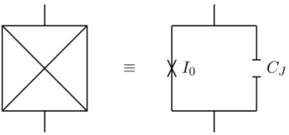
The physics inside Josephson junctions. In this context the famous Josephson re- lations are derived. Starting point is the composition of a Josephson junction. Such a junction consists of two generic superconducting electrodes that are connected by a small tunnelling barrier. This device is illustrated in Fig. 1.4, where the cross represents the barrier and the upper and lower part symbolise the superconductors. This composition has a capacitanceC_J, which is also visualised in the figure.

≡ I0 CJ

Figure 1.4: Josephson junction with critical current I0 and junction capacitanceCJ.

Following the theory of Feynman [FLS65], the system is considered as a two-level quantum mechanical system, describing Cooper pairs. Now the voltage U is applied to the junction, such that the energy-levels of a given Cooper pair are separated by 2eU. The fundamental dynamics of the system is described by Schr¨odinger’s equation i~∂t|ψ(t)i = ˆH|ψ(t)i with a specific Hamilton operator ˆH. As only discrete states, labelled |ψ_ki with k = 1,2, are allowed in the model, the wavefunction of the system is expanded into a series |ψ(t)i = P

kc_k(t)|ψ_ki with complex and time depending coefficientsck(t). Inserting this ansatz into the Schr¨odinger equation leads to differential equations for all coefficients c_k(t),

i~ d

dtc_k(t) =X

l

H_klc_l(t), (1.30)

with matrix elements Hlk=hψl|Hˆ |ψ_ki.The energy scale of the system is chosen in a way, such that the diagonal elements of the matrixH areH11 = eU andH22 = −eU. The tunnelling coefficient in this model is given byH₁₂ = K. Using this notation, the

(24)

CHAPTER 1. THE POINT OF INTEREST two differential equations in Eq. (1.30) are

i~ d

dtc₁(t) =eU c₁(t) +Kc₂(t) and i~ d

dtc₂(t) =Kc₁(t)−eU c₂(t). (1.31) The absolute square |c_k(t)|² is normalised in a way, such that |c_k(t)|² ≡ ns(t) is the superconducting electron density in the junction. As the amplitude of a coefficientc_k(t) is fixed by this condition, each coefficient can only acquire an additional phasefactor θ_k(t), leading to

c_k(t) =p

n_s(t)e^iθ^k^(t). (1.32)

Inserting this ansatz in the differential equation above reveals a set of three differential equations forns(t),θ1(t) and θ2(t) given by

d

dtns(t) = 2Kns(t)

~ sinφ(t), (1.33a)

d

dtθ1(t) =−K

~ cosφ(t)−eU

~ , (1.33b)

d

dtθ₂(t) =−K

~ cosφ(t) +eU

~ . (1.33c)

Here, the phase differenceφ(t) =θ1(t)−θ2(t) is introduced. Remember that the superconducting electron density is given byns(t). Obviously, the current through the tunnel junction is proportional to the time derivative of this density,

I(t) = d

dtns(t). (1.34)

Accordingly, Cooper pairs start to leave one of the superconducting electrodes. This effect is immediately compensated by the arrival of new electrons from an external source, as the junction is part of a closed electric circuit. Consequently, the density n_s(t) remains constant due to electroneutrality of the system as a whole. In this way the first fundamental Josephson relation,

I(t) =I₀sinφ(t), (1.35)

is derived. It describes the time dependence of the current through the junction. Now the phase differenceφ(t) is investigated. The second fundamental Josephson relation,

∂tφ(t) = 2eU

~ , (1.36)

can easily be derived from Eq. (1.33b) and Eq. (1.33c). Finally, the Josephson energy is given as

E(t) =

t

Z

−∞

dτ I(τ)U =−E_Jcosφ(t) (1.37)

(25)

1.3. PHYSICAL REALISATIONS OF QUBITS withEJ =^~I⁰/2e.

There are two common ways of creating qubits by the use of Josephson junctions. In the following paragraph the construction of a charge qubit corresponding to the work of Bouchiat [BVJD98] is explained. An alternative implementation is given by flux qubits, which are found e.g. in reference [CNHM03].

Construction of a charge qubit. Construct a circuit with an applied gate voltage U_g and implement a Josephson junction and an additional capacitor with capacity Cg, as illustrated in Fig. 1.5. There is a part of the circuit which is isolated by the capacitor on

U_g Cg

Figure 1.5: Charge qubit with gate voltage Ug, a capacitor having capacity Cg and a Josephson junction.

the one and the junction on the other side. A certain number of Cooper pairs is within this island. This number can be controlled by changing the gate voltage.

The first step is the derivation of the model’s Hamiltonian. One contribution to the Hamiltonian is the charging energy E_c =^e²/2(Cg+CJ), which is needed to transport electrons into the qubit area. The gate charge number is given asn_g =^C^g^U^g/2e.Together with the Josephson energy, derived in Eq. (1.37), the system’s Hamiltonian is

Hˆ = 4E_c(n−n_g)²−E_Jcosφ , (1.38) wherenis the particle-number operator of the isolated area. As particle-number operator and phase operator are conjugated variables, according to the Susskind-Glogower formalism [Lyn95], the commutator is [φ, n] = i. For the phase it is known that e^±iφ|ni=|n±1i.Now the Hamiltonian is given by

Hˆ =X

n

4Ec(n−ng)²|nihn| − EJ

2 (|nihn+ 1|+|n+ 1ihn|)

. (1.39) This Hamiltonian determines the complete physics of the specified device.

In the following an explicit construction of a qubit within this model is outlined. A qubit consists of two states. For this purpose the ground and first excited state are selected. The corresponding particle-number operator is given by

n= 0 0

0 1

= 1−Z

2 . (1.40)

(26)

This operator is inserted into the Hamiltonian above. Within the given sum all terms that include other states than the ground and first exited state are neglected. Finally, after rescaling, the Hamiltonian has the form

Hˆ =−2E_c(1−2ng)Z−EJ

2 X . (1.41)

In a physical implementation of a charge qubit, noise occurs up to the fact that the gate voltageU_g fluctuates. Building a lattice, with an index mthat labels different sites, the free Hamiltonian of the system is

Hˆ₀ =−X

m

2E_c(1−2n_g,m)Z_m. (1.42) LetδUm be the difference of the voltage to the original gate voltage. Than, the interaction Hamiltonian is given by

HˆI =−X

m

EJ

2 Xm−2CgδUm

e Zm. (1.43)

Now an explicit choice for the noise is taken and the corresponding spectral parameter s of the spectral density is calculated. Assuming δUm occurs by a change of the flux through the circuit caused by thermal photons. Then, the voltage is given by

δU_m= ˙Φ_m =−

2π

Z

0

dsγ˙_m(s)·E(γ_m(s), t) (1.44) with flux Φ, electric fieldE and circuit parametrisation γ. Taking a circuit in form of a circle of radiusL, one possible parametrisation is

γ_m(s) =ame3+L(cos(s)e1+ sin(s)e2). (1.45) If a kind of dipole approximation is applied to this setting such that the electromagnetic field is assumed to be constant over the area of each circuit, the spectral parameter of the spectral density, cf. Eq. (1.10), iss= 5.

Note that there are other kinds of noise in these junctions and their influence seems to be even more disturbing than the effects which occur due to the above mentioned coupling. As these charge qubits are normally part of a larger solid crystal there are impurities around, which interact with the qubit. Each of these fluctuators causes a telegraph noise, resulting in a 1/f-noise. A description to this phenomenon is given in [MSS03] and references therein. This setting cannot be mapped to a spin-boson model such that it is not further discussed within the scope of this work.

(27)

1.3. PHYSICAL REALISATIONS OF QUBITS 1.3.3 Qubits with quantum dots

Quantum dots are systems of some to a few hundred electrons which are spatially confined in a region of nanometre scale. One possible realisation of a quantum dot is due to semiconductors. By the choice of different material layers an effective two-dimensional electron gas is formed in these devices. With additional gates on the device a potential is created to isolate the electrons in a certain area, the quantum dot. The energy levels of such dots are quantised due to the confinement of the electrons. In the following consideration a quantum dot with a single confined electron is investigated. The ground- state|gi ≡ |1i and the first excited state|ei ≡ |0i of such an electron form the qubit.

This concept of quantum computation with quantum dots was introduced by Loss and DiVincenzo [LD98].

Introduction to electron-phonon interactions. Starting point is a slightly generalised setting with a finite amount of electrons in the quantum dot and not just a single one. A typical kind of interaction with an environment of these electrons is due to phonons, as it is pointed out in this section. For reference see the book of Mahan [Mah81]. Starting point is the Hamiltonian

Hˆ = ˆH_p+ ˆH_e+ ˆH_ei, (1.46) where electrons interact via phonons with their lattice ions. Thereby, the free Hamilto- nian of a phononic environment is

Hˆ_p =X

k,λ

ω_k,λ

a^†_kλa_kλ+1 2

. (1.47)

Here,a^†_kλand a_kλ are bosonic creation and annihilation operators of thek^th mode with polarisation λ. The energy of a modek is given by ~ωk. Another contribution to ˆH is due to electrons. Their free Hamiltonian is given by the sum of their kinetic energy and coulomb repulsion potential as

Hˆ_e=X

i

p²_i 2m +e²

2 X

i6=j

1

r_ij . (1.48)

In this equation,m is the mass of a electron and r_ij is the distance between thei^th and j^th electron. The remaining part of ˆH is the interaction Hamiltonian. This interaction of the confined electrons with their lattice ions is given by

Hˆ_ei =X

i

V˜(r_i). (1.49)

Here, ri is the position of the i^th electron and ˜V is the effective potential which is produced by all lattice ions. Now these effective potentials are investigated. The i^th electron at positionr_i and its interaction with thej^th lattice ion is observed. Let R_j be

(28)

the position of the j^th lattice ion. Consequently, the interaction between electron and ion is given by a potentialVei(ri−Rj). As the effective potential ˜V for thei^th electron is given by the interaction with all lattice ions it reads

V˜(ri) =X

j

Vei(ri−Rj). (1.50)

Now the position of thej^thion is given by its equilibrium valueR^eq_j and the displacement from its origin Qj as Rj =R^eq_j +Qj. The above introduced potentialVei is, assuming a small displacement, expanded into a Taylor series,

Vei(ri−Rêq_j −Qj) =Vei(ri−Rêq_j ) +Qj· ∇V_ei(ri−Rêq_j ) +O(Q²). (1.51) The first contributing term is the one linear inQ, as the constant termP

jVei(ri−R^eq_j ) can be neglected. This neglection of the constant term is formally achieved by a rescaling of the Hamiltonian. A rescaling is possible as the constant term corresponds to the potential energy of the electrons if the ions are at their equilibrium position. Concluding, the effective potential for a electron-phonon interaction is given by

V˜(r) =X

j

Q_j· ∇V_ei(r−R^eq_j ), (1.52) where higher orders of the expansion are neglected. Now the potentialVei(r) is expanded into a Fourier series over phononic modeskgiven byV_ei(r) = _N¹ P

kV_ei(k)e^ik·r,whereN is the number of interacting ions. Its gradient in the Fourier transformed form is easily calculated to be∇V_ei(r) = _Nⁱ P

kkVei(k)e^ik·r.Inserting this result into Eq. (1.52) gives V˜(r) = i

N X

k

kV_ei(k)e^ik·r

!

·



 X

j

Q_je^−ik·R^eq^j



 . (1.53)

The summation over all modes k is replaced by two summations over q and G with k =q+G. Here, G is a reciprocal lattice vector and q lies within the first Brillouin zone. Therefore, G·R^eq_j is a multiple of 2π and accordingly the effective potential is given by

V˜(r) =





√i N

X

q,G

kVei(k)e^ik·r



·





√1 N

X

j

Qje^−iq·R^eq^j



 . (1.54)

The last part is identified to be the Fourier transformed of Qq, given by Q_q = ^√¹

N

P

jQ_je^−iq·R^eq^j . At this point an ansatz for the coefficients Q_q, in the form of

Qq=−i s

~

2M ω_qξq(a_q+a^†_−q), (1.55)

(29)

1.3. PHYSICAL REALISATIONS OF QUBITS is inserted. Here, M is the mass of an ion and ξq is the polarisations of the mode q.

Volume ν and the density of the solid ρ are introduced by M N = ρν such that the effective potential reads

V˜(r) =−X

q,G

s

~ 2ρνωq

(q+G)V_ei(q+G) ˆξ_q(a_q+a^†_−q)e^i(q+G)·r. (1.56) Having the effective potential provides full information about the interaction Hamilto- nian in Eq. (1.49).

Two different regimes are discussed in the following. First the deformation potential, occurring due to the coupling to acoustical phonons is presented. Afterwards the piezoelectric interaction is outlined.

The deformation potential. The deformation potential is a coupling to acoustical phonons in the long-wavelength limit of Eq. (1.56). This limit corresponds to small norms ofq+G. Hence, only the part withG= 0 remains, as other terms are obviously of shorter wavelengths. The potential is replaced by the deformation constant D, as V_ei(q) → D in the considered limit of long wavelength. Assuming a nondegenerated band at long wavelength only longitudinal phonons are important, such that ˆξq→q. Inˆ this limit the interaction Hamiltonian is

Hˆei=X

l

DX

q

s

~

2ρνω_q|q|(a_q+a^†_−q)e^iq·r^l. (1.57)

Piezoelectric interactions. Piezoelectric interactions are the interactions of a solid to an electric field. The microscopic effect of this interaction is that a crystal is squeezed if an electric field is applied and vice versa. The analysis of this piezoelectric interaction is adduced by a short excursion to the stress of a solid. The stress S is defined as the symmetric derivative of the displacement field Q,

S_ij = 1 2

∂Q_i

∂rj

+∂Q_j

∂ri

= 1 2

X

q

s

~ 2ρνωq

(ξ_iq_j +ξ_jq_i)(a_q+a^†_−q)e^iq·r. (1.58) Note that Q_i in this case is the i^th component of the field Q ≡ Q(r) and not the displacement Q at the position of the i^th ion. The Fourier transformed displacement Q(r) = ^√¹

N

P

qQ_qe^iq·r is inserted, having Fourier coefficients Q_qwithin the sum that were already introduced in Eq. (1.55). For a given stress S_ij on the crystal the electric field is proportional to the stress,

E_l=X

i,j

M_ijlSij, (1.59)