New relevance and significance measures to replace p-values Werner A. Stahel

New relevance and significance measures to replace p-values

Werner A. Stahel^1*

1Seminar for Statistics, ETH, Zurich, Switzerland

* stahel@stat.math.ethz.ch

Abstract

The p-value has been debated exorbitantly in the last decades, experiencing fierce critique, but also finding some advocates. The fundamental issue with its misleading interpretation stems from its common use for testing the unrealistic null hypothesis of an effect that is precisely zero. A meaningful question asks instead whether the effect isrelevant. It is then unavoidable that a threshold for relevance is chosen. Considerations that can lead to agreeable conventions for this choice are presented for several commonly used statistical situations. Based on the threshold, a simple quantitative measure of relevance emerges naturally. Statistical inference for the effect should be based on the confidence interval for the relevance measure. A classification of results that goes beyond a simple distinction like

“significant / non-significant” is proposed. On the other hand, if desired, a single number called the “secured relevance” may summarize the result, like the p-value does it, but with a scientifically meaningful interpretation.

1 Introduction

The p-value is arguably the most used and most controversial concept of applied statistics. 2

Blumeet al.[1] summarize the shoreless debate about its flaws as follows: “Recurring 3

themes include the difference between statistical and scientific significance, the routine ⁴ misinterpretation of non-significant p-values, the unrealistic nature of a point null ⁵ hypothesis, and the challenges with multiple comparisons.” They nicely collect 14 citations, ⁶ and I refrain from repeating their introduction here, but complement the analysis of the ⁷ problem and propose a solution that both simplifies and extends their’s. ⁸ The basic cause of the notorious lack of reliability of empirical research, notably in parts ⁹ of social and medical science, can be found in the failure to ask scientific questions in a ¹⁰ sufficiently explicit form, and the p-value problem is intrinsically tied to this flaw. Here is my ¹¹

argument. ¹²

Most empirical studies focus on the effect of some treatment, expressed as the difference ¹³ of a target variable between groups, or on the relationship between two or more variables, ¹⁴ often expressed with a regression model. Inferential statistics needs a probabilistic model ¹⁵ that describes the scientific question. Usually, this is a parametric model in which the effect ¹⁶ of interest appears as a parameter. The question is then typically specified as: “Can we 17

prove that the effect is not zero?” 18

The Zero Hypothesis Testing Paradox. This is, however, not a scientifically ¹⁹ meaningful question. When a study is undertaken to find some difference between groups or ²⁰ some influence between variables, thetrue effect—e.g., the difference between two within ²¹ group expected values—will never be precisely zero. Therefore, the strawman null hypothesis ²² of zero true effect (the “zero hypothesis”) could in almost all reasonable applications be ²³ rejected if one had the patience and resources to obtain enough observations. Consequently, ²⁴

January 2, 2021 1/22

the question that is answered mutates to: “Did we produce sufficiently many observations 25

to prove the (alternative) hypothesis that was true on an apriori basis?” This does not seem ²⁶ to be a fascinating task. I call this argument the “Zero Hypothesis Testing Paradox.” The ²⁷ problem with the p-value is thus that it is the output of testing an unrealistic null hypothesis ²⁸ and thereby answers a nonsensical scientific question. (Note that the proposal to lower the ²⁹ testing level from5 % to0.5 %by Benjaminet al.[2] is of no help in this respect.) ³⁰ A sound question about an effect is whether it is large enough to berelevant. In other ³¹ words: Without the specification of a threshold of relevance, the scientific question is void. ³² Scientists have gladly avoided the determination of such a threshold, because they felt ³³ that it would be arbitrary, and have jumped on the train of “Null Hypothesis Significance ³⁴ Testing,” that was offered cheaply by statistics. Let us be clear: Avoiding the choice of a ³⁵ relevance threshold means avoiding a scientifically meaningful question. ³⁶ Given the relevance threshold, the well-known procedures can be applied not only for ³⁷ testing the null hypothesis that the effect is larger than the threshold against the alternative ³⁸ that it is smaller, but also vice versa, proving statistically that the effect is negligible. The 39

result can of course also be ambiguous, meaning that the estimate is neither significantly 40

larger nor smaller than the threshold. I introduce a finer distinction of cases in Section 2.3. ⁴¹ These ideas are well-known under the heading of equivalence testing, and similar ⁴² approaches have been advocated in connection with the p-value problem, like the “Two ⁴³ One-Sided Tests (TOST)” of Lakens [3], the “Second Generation p-value (SGPV)” by ⁴⁴ Blumeet al.[1], or the “Minimum Effect Size plus p-value (MESP)” by Goodmanet al.[4]. ⁴⁵ The threshold has been labelled “Smallest Effect Size Of Interest (SESOI)” or “Minimum ⁴⁶ Practically Significant Distance (MPSD).” I come back to these concepts in Section 2.2. ⁴⁷ Using confidence intervals instead of p-values or even “yes-no” results of null hypothesis ⁴⁸ tests provides the preferable, well-known alternative to null hypothesis testing for drawing ⁴⁹ adequate inference. Each reader can then judge a result by checking if his or her own ⁵⁰ threshold of relevance is contained in the interval. Providing confidence intervals routinely ⁵¹ would have gone a long way to solving the problem. I come back to this issue in the ⁵²

Discussion (Section 6). ⁵³

Most probably, the preference to present p-values rather than confidence intervals is due 54

to the latter’s slightly more complicated nature. In their usual form, they are given by two 55

numbers that are not directly comparable between applications. I will define a single ⁵⁶ number, which I call “significance,” that characterizes the essence of the confidence interval ⁵⁷

in a simple and informative way. ⁵⁸

In “ancient” times, before the computer produced p-values readily, statisticians examined ⁵⁹ the test statistics and then compared them to tables of “critical values.” In the widespread ⁶⁰ case that the t test was concerned, they used the t statistic as an informal quantitative ⁶¹ measure of significance of an effect by comparing it to the number 2, which is approximately ⁶² the critical value for moderate to large numbers of degrees of freedom. This will also shine ⁶³

up in the proposed significance measure. ⁶⁴

Along the same line of thought, a simple measure of relevance will be introduced. It ⁶⁵ compares the estimated effect with the relevance threshold. The respective confidence ⁶⁶ interval is used to distinguish the cases mentioned above, and a single value can be used to ⁶⁷ characterize the result with the same simplicity as the p-value does it, but with a much ⁶⁸

more informative interpretation. 69

2 Definitions

The simplest case for statistical inference is the estimation of a constant based on a sample ⁷¹ of normal observations. It directly applies to the estimation of a difference between two ⁷² treatments using paired observations. I introduce the new concepts first for this situation. ⁷³ The problem of assessing a general parameter as well as the application of the concepts for ⁷⁴

January 2, 2021 2/22

typical situations—comparison of two or more samples, estimation of proportions, regression 75

and correlation—will be discussed in Section 3. ⁷⁶

2.1 The generic case

Consider a sample ofnstatistically independent observationsYi with a normal distribution, ⁷⁸ Yi∼ N ϑ, σ²

. (1)

The interest is in knowing whetherϑis different from0 in a relevant manner, where 79

relevance is determined by the relevance thresholdζ >0. Thus, I want to summarize the 80

evidence for the hypotheses 81

H0: ϑ≤ζ , H1: ϑ > ζ .

(The symbolζ, pronounced “zeta,” delimits the “zero” hypothesis.) ⁸² One sided. I consider a one-sided hypothesis here. In practice, only one direction of the 83

effect is usually plausible and/or of interest. Even if this is not the case, the conclusion 84

drawn will be one-sided: If the estimate turns out to be significant according to the ⁸⁵ two-sided test for 0 effect, then nobody will conclude that “the effect is different from zero, ⁸⁶ but we do not know whether it is positive or negative.” Therefore, in reality, two one-sided ⁸⁷ tests are conducted, and technically speaking, a Bonferroni correction is applied by using the ⁸⁸ levelα/2 = 0.025 for each of them. Thus, I treat the one-sided hypothesis and use this ⁸⁹

testing level. ⁹⁰

The point estimate and confidence interval are ⁹¹

ϑb=Y = ¹_nP

iYi, CIϑ=ϑb±ω ,b ωb=q

qV /n ,b (2)

where Vb is the empirical variance of the sample,Vb = _n−1¹ P

i(Yi−Y)², andqis the ⁹² 1−α/2 = 0.975quantile of the appropriatetdistribution. Thus, ωbis half the width of the ⁹³ confidence interval and equals the standard error, multiplied by the quantile. ⁹⁴ In general problems involving a single effect parameter, the estimated effect usually ⁹⁵ follows approximately a normal distribution, and these concepts are easily generalized, see 96

Section 3. 97

Significance. The proposed significance measure compares the difference between the ⁹⁸ estimated effect and the relevance threshold with the half width of the confidence interval, ⁹⁹

Sigζ = (ϑb−ζ)/ω .b (3)

The effect is statistically significantly larger than the threshold if and only if Sig_ζ >1. 100

Significance can also be calculated for the common test for zero effect, Sig₀=ϑ/b ω.b ¹⁰¹ This quantity can be listed in computer output in the same manner as the p-value is given in ¹⁰² today’s programs, without a requirement to specifyζ. It is much easier to interpret than the ¹⁰³ p-value, since it is, for a given precision expressed byω, proportional to the estimated effectb ¹⁰⁴ ϑ. Furthermore, a standardized version of the confidence interval for the effect is Sigb ₀±1, ¹⁰⁵

Sig₀±1 =ωbCIϑ, CIϑ=ϑb 1±1/Sig₀ .

Nevertheless, it should be clear from the Introduction that Sig₀ should only be used with ¹⁰⁶

extreme caution, since it does not reflect relevance. ¹⁰⁷

January 2, 2021 3/22

Relevance. An extremely simple and intuitive quantitative measure of relevance is the 108

effect, expressed inζ units, Rl=ϑ/ζ. Its point and interval estimates are ¹⁰⁹

Rle=ϑ/ζ ,b CIRl=CIϑ/ζ . (4)

I also introduce the “secured relevance” as the lower end of the confidence interval, ¹¹⁰ Rls=Rle−ωb^∗, ωb^∗=ω/ζb

and the “potential relevance” Rlp=Rle+ωb^∗. The effect is called relevant if Rls>1, that ¹¹¹ is, if the estimated effect is significantly larger than the threshold. ¹¹²

The estimated relevance Rle is related to Sigζ by ¹¹³

Sigζ = (Rle−1)/ωb^∗ , Rle=Sigζωb^∗+ 1.

Fig 2 shows several cases of relations between the confidence interval and the effects0 ¹¹⁴ andζ, which can be translated into categories that help interpret results, see Section 2.3. 115

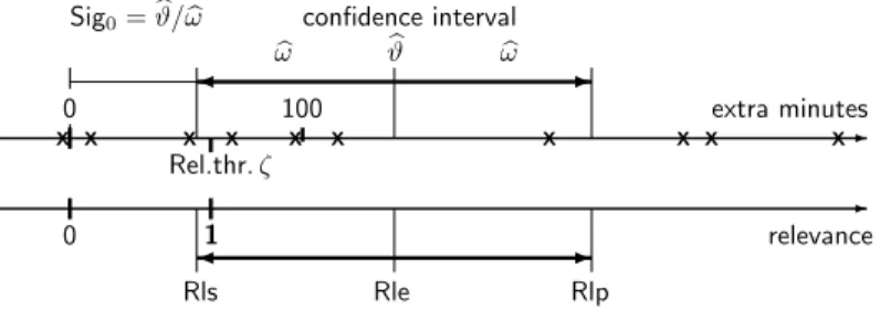
Example: Student’s sleep data. Student [5] illustrated his t-test with data measuring ¹¹⁶ the extra sleep evoked by a sleep enhancing drug in 10 patients. The numbers in minutes ¹¹⁷ are−6,6,48,66,96, 114,204,264,276,330. Their mean isϑb=Y = 140. The p-value ¹¹⁸ for testing the hypothesis of no prolongation is0.5 %and the confidence interval extends ¹¹⁹ from54to226. The zero significance is obtained fromV = 14,432,n= 10andq= 2.26 ¹²⁰ withωb= 2.26p

14,432/10 = 86as Sig0 = 140/86 = 1.63. 121

If the relevance threshold is one hour,ζ= 60, of extra sleep then Sig_ζ = 80/86 = 0.93, ¹²² and the gain is not significantly relevant. This is also seen when calculating the relevance ¹²³ and its confidence interval, Rle= 140/60 = 2.33and Rls= 2.33−86/60 = 54/60 = 0.90, ¹²⁴ Rlp= 2.33 + 86/60 = 226/60 = 3.76. It remains therefore unclear whether the sleep ¹²⁵ prolongation is relevant. Fig 1 shows the results graphically. ¹²⁶

extra minutes-

0 100

Rel.thr.ζ

ωb ϑb ωb - Sig0=ϑ/bωb confidence interval

- relevance

0 1 -

Rle

Rls Rlp

X X X X X X X X X X

1

127

Fig 1. Estimate, confidence interval and relevance for the sleep data

2.2 Related concepts

Two one-sided tests (TOST). Lakens [3] focusses on testing for a negligible effect, ¹²⁹ advocating the paradigm of equivalence testing. He considers an interval of values that are ¹³⁰ negligibly different from the point null hypothesis, also called a “thick” or “interval ¹³¹ null” [4], [1]. If this interval is denoted as|ϑ| ≤ζ, there is a significantly negligible effect if ¹³² both hypothesesϑ > ζ andϑ < −ζare rejected using a one-sided test for each of them. A 133

respective p-value is the larger of the p-values for the two tests. 134

I have argued for a one-sided view of the scientific problem. With this perspective, the ¹³⁵ idea reduces to theone one-sided test for a negligible effect with significance measure ¹³⁶

−Sig_ζ. ¹³⁷

January 2, 2021 4/22

Second Generation P-Value. The “Second Generation P-Value” SGPVPδ has been 138

introduced by Blumeet al.[1, 6]. In the present notation,ζ is theirδ. The definition ofPζ ¹³⁹

starts from considering the lengthOof the overlap of the confidence interval with the ¹⁴⁰ interval defined by the composite null hypothesisH0. Assume first that ϑ >b 0. Then, the ¹⁴¹ overlap measuresO= 2ωbif the confidence interval contains the “null interval,” that is, if ¹⁴² ϑb+ω < ζb , and otherwise,O=ζ−(bϑ−ω), orb 0 if this is negative. ¹⁴³ The definition ofPζ distinguishes two cases based on comparingωbto the thresholdζ. If ¹⁴⁴ b

ω <2ζ,Pζ = 0if there is no overlap, andPζ = 1for complete overlap,O= 2ω. Inb ¹⁴⁵ between, the SGPV is the overlap, compared to the length of the confidence interval, ¹⁴⁶

Pζ = O

2ωb = ζ−(bϑ−ω)b

2ωb = ζ−ϑb

2ωb +¹₂ = ¹₂ 1−Sig_ζ .

In this case, then,Pζ is a rescaled, mirrored, and truncated version of the significance atζ. ¹⁴⁷ Here, I have neglected a complication that arises when the confidence interval covers ¹⁴⁸ values below−ζ. The definition ofPζ starts from a two-sided formulaton of the problem, ¹⁴⁹ H0: |ϑ|< ζ. Then, the confidence interval can also cover values below−ζ. In this case, ¹⁵⁰

the overlap decreases andPζ changes accordingly. ¹⁵¹

The definition of Pζ changes if the confidence interval is too large, specifically, if its ¹⁵² length exceeds2ζ. This comes again from the fact that it was introduced with the ¹⁵³ two-sided problem in mind. In order to avoid small values ofPζ caused by a large ¹⁵⁴ denominator2ωbin this case, the length of the overlapOis divided by twice the length2ζof ¹⁵⁵ the “null interval,” instead of the length of the confidence interval,2ω,b Pζ =O/(4ζ). Then, ¹⁵⁶ Pζ has a maximum value of 1/2, which is a deliberate consequence of the definition, as this 157

value does not suggest a “proof” ofH0. For a comparison of the SGPV with TOST, see [7]. 158

If the overlap is empty,Pζ = 0. In this case, the concept of SGPV is supplemented with ¹⁵⁹

the notion of the “δgap,” ¹⁶⁰

Gap_ζ = (bϑ−ζ)/ζ=Rle−1.

Since the significance and relevance measures are closely related to the Second ¹⁶¹ Generation P-Value and theδgap, one might ask why still new measures should be ¹⁶²

introduced. Here is why: ¹⁶³

• An explicit motivation for the SGPV was that it should resemble the traditional ¹⁶⁴ p-value by being restriced to the 0-1 interval. I find this quite undesirable, as it ¹⁶⁵ perpetuates the misinterpretation ofP as a probability. Even worse, the new concept ¹⁶⁶ is further removed from such an interpretation than the old one, for which the ¹⁶⁷ problem “Find a correct statement including the terms p-value and probability” still 168

has a (rather abstract) solution. 169

• The new p-value was constructed to share with the classical one the property that ¹⁷⁰ small values signal a large effect. This is a counter-intuitive aspect that leads to ¹⁷¹ confusion for all beginners in statistics. In contrast, larger effects lead to larger ¹⁷²

significance (and, of course, larger relevance). ¹⁷³

• Taking these arguments together, the problems with the p-value are severe enough to ¹⁷⁴ prefer a new concept with a new name and more direct and intuitive interpretation ¹⁷⁵ rather than advocating a new version of p-value that will be confused with the ¹⁷⁶

traditional one. ¹⁷⁷

• The definition of the SGPV is unnecessarily complicated, since it is intended to ¹⁷⁸ correspond to the two-sided testing problem, and only quantifies the undesirable case ¹⁷⁹ of ambiguous results. It deliberately avoids to quantify the strength of evidence in the ¹⁸⁰

two cases in which either H0 orH1 is accepted. 181

January 2, 2021 5/22

2.3 Classification of results

There is a wide consensus that statistical inference should notbe reported simply as ¹⁸³

“significant” or “non-significant.” Nevertheless, communication needs words. I therefore ¹⁸⁴ propose to distiguish the cases that the effect is shown to be relevant (Rlv), that is, ¹⁸⁵ H1:ϑ > ζ is “statistically proven,” or negligible (Ngl), that is,H0:ϑ≤ζ is proven, or the ¹⁸⁶ result is ambiguous (Amb), based on the significance measure Sig_ζ or on the secured and ¹⁸⁷ potential relevance Rls and Rlp (Rls>1 for Rlv, Rlp<1for Ngl and Rls≤1≤Rlp for ¹⁸⁸

Amb). ¹⁸⁹

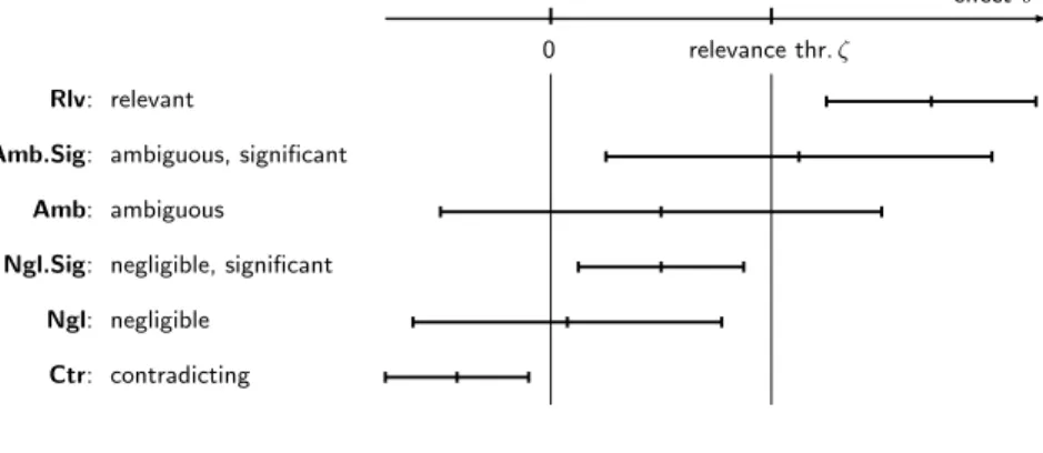
For a finer classification, the significance for a zero effect, Sig₀, is also taken into ¹⁹⁰ account. This may even lead to a contradiction (Ctr) if the estimated effect is significantly ¹⁹¹ negative. Fig 2 shows the different cases with corresponding typical confidence intervals, ¹⁹² and Table 1 lists the respective significance and relevance ranges. Similar figures have ¹⁹³ appeared in [1, Fig. 2] and [4, Fig. 1] and before, with different interpretations. ¹⁹⁴

effect-ϑ

0 relevance thr.ζ

Rlv: relevant

Amb.Sig: ambiguous, significant Amb: ambiguous

Ngl.Sig: negligible, significant Ngl: negligible

Ctr: contradicting

1

195

Fig 2. Classification of cases based on a confidence interval and a relevance threshold

Table 1. Classification of cases defined by ranges of significance and relevance measures. s andrare the place holders for the column headings.

Case Sig0 Sigζ Rls Rlp

Rlv s >>1 s >1 r >1 r >>1 Amb.Sig s >1 −1< s <1 0< r <1 r >1

Amb −1< s <1 −1< s <1 r <0 r >1 Ngl.Sig s >1 s <−1 0< r <1 0< r <1

Ngl −1< s <1 s <−1 r <0 0< r <1 Ctr s <−1 s <<−1 r <<0 r <0

January 2, 2021 6/22

3 Generalization and more models

3.1 General model and two-sample problem

Let us now discuss a general parametric model. To make the notation transparent, the 198

two-sample problem is discussed in parallel as an example. 199

Considernstatistically independent observations following the parametric model 200

Yi∼ F θ, φi;xi

, (5)

whereθis the parameter of interest,φi denotes nuisance parameters, and the distributionF 201

may vary between observations depending on covariatesxi. These variables may be ²⁰²

multidimensional. ²⁰³

The model for comparing two treatments arises when xi= 1if observationi received ²⁰⁴ treatment1, andxi= 0otherwise;θis the difference of expected values between the two ²⁰⁵ groups; and the nuisance parameters are the expected valueφ⁽¹⁾=µ0ofYi for treatment ²⁰⁶ k= 0 and the standard deviation of the observations,φ⁽²⁾=σ. Then, ²⁰⁷

Yi∼ N µ0+θxi, σ² .

The problem is to draw inference about the effect θ. There is a “null value”θ0and a 208

thresholdζ for a relevant effect. For ease of notation, assumeζ >0. 209

Inference is based on an estimatorθbofθ. Assume that its distribution is approximately ²¹⁰

(multivariate) normal, ²¹¹

θb≈∼ Np(θ,V/n) , (6)

where the “single observation” variance-covariance matrixVmay depend on all nuisance ²¹² parametersφi and design vectorsxi, i= 1, ..., n, andpis the dimension ofθ. It may also ²¹³ depend on the parameter of interest,θ, but this case needs additional discussion. These ²¹⁴ assumptions usually hold for the Maximum Likelihood Estimator of[θ, φ],V being the ”θ ²¹⁵ part” of the inverse Fisher Information of a single observation. ²¹⁶ In the two samples problem withn0 observations in groupk= 0andn1, in groupk= 1, ²¹⁷

bθ = _n¹₁P

iYixi−_n¹

0

P

iYi(1−xi) V = (1/ν0+ 1/ν1)σ², νk =nk/n .

Effect scale. In several models, it appears useful to consider a transformed version of the 218

parameter of interest as the effect, since the transformation leads to a more generally ²¹⁹ interpretable measure and may have more appealing properties, as in the next subsection. ²²⁰ Therefore, the original parameter of interest is denoted asθ or as popular in the model, and ²²¹ the transformed version will be considered as the effect,ϑ=g(θ). ²²² In order to obtain a standardized version of an effect measure that does not depend on ²²³

units of measurement, the effect can be standardized, ²²⁴

ϑ=θ.√

V

in the one-dimensional case. (For the mulitvariate case, see Section 3.6.) Note that the ²²⁵ single observation variance is used here, which makes the definition a parameter of the ²²⁶ model, independent of the number of observations. It still depends on the estimator of the ²²⁷ parameter (and the design in regression models, see below) throughV. One may therefore ²²⁸ use the inverse Fisher information for the effect, which equals the variance of the Maximum ²²⁹ Likelihood Estimator, instead of theV defined by the estimator actually used. 230

January 2, 2021 7/22

If the variance depends on the effect parameter, this standardization is of limited value. 231

Therefore, a variance stabilizing transformation may be appropriate. If V is constant, the ²³²

confidence interval for the standardized effect is ²³³

ϑb±q√ n ,

where qis the appropriate quantile of the normal or a t distribution. ²³⁴ In the case of two samples, a very popular way to standardize the difference between the ²³⁵

groups is Cohen[8]’sd ²³⁶

d=θ σ .

The standardized effectϑis related todby ²³⁷

ϑ=dp

1/ν0+ 1/ν1=d√ ν0ν1.

If the two groups are equally frequent,ν0=ν1= 1/2, thend= 2ϑ. ²³⁸ Cohen’sdand the effectϑcompare the difference between the groups to the variationσ ²³⁹ of the target variable within groups. This makes sense ifσmeasures the natural standard ²⁴⁰ variation between observation units. It is not well justified if it includes measurement error, ²⁴¹ since this would change if more precise measurements were obtained, for example, by ²⁴² averaging over several repeated measurements. In this case, the standardized effect is not ²⁴³ defined by the scientific question alone, but also by the study design. ²⁴⁴ Even thoughdandϑhave been introduced in the two samples framework, they also ²⁴⁵ apply to a single sample, since the effect in this case is the difference between its expected ²⁴⁶ value and a potential population that has an expectation of zero. Remember that the effect ²⁴⁷ and its threshold are defined as a function of parameters (a single one in this case), not of ²⁴⁸

their estimates. ²⁴⁹

3.2 Proportions

When a proportion is estimated, the model is, using Bto denote the binomial distribution, ²⁵¹ Yi ∼ B(1, p) , pb=S/n , S=P

iYi∼ B(n, p) b

p ≈∼ N(p, Vp/n) , Vp=p(1−p).

For this model, the varianceVp depends on the parameter of interest. As a consequence, ²⁵² the confidence intervals derived from the asymptotic approximation are not suitable for ²⁵³ small to moderate sample sizes—more precisely, for smallnporn(1−p). Exact confidence ²⁵⁴ intervals are well-known and resolve the problem. However, choosing a relevance threshold ²⁵⁵ needs more attention. It may be plausible to say that a difference of0.05is relevant ifpis ²⁵⁶ around1/2, but such a difference is clearly too high ifpis itself around0.05or below. Thus, 257

the relevance threshold should depend on the effect itself. The choice of a relevance 258

threshold is discussed in Section 4. ²⁵⁹

Variance stabilizing transformation. A variance stabilizing transformation helps to ²⁶⁰

make the general procedures more successful. Here, ²⁶¹

ϑ=g(p) = asin(√

p)/ (π/2)

is the useful transformation. (The division byπ/2 entails a range from0to1.) It leads to ²⁶² ϑb=g(S/n)≈∼ N(ϑ, V /n) , V = 1/π².

January 2, 2021 8/22

Risk. Risks usually have low probabilities of occurring. Good practice focusses on 263

logarithmically transformed risks, even more clearly when comparing or modelling them: ²⁶⁴ When a treatment changes a risk, the effect is naturally assessed in terms of a percentage ²⁶⁵ change it entails. This translates into a change on the log scale that is independent of the ²⁶⁶ probabilityp. Thus, the effect measure should beϑ= log(p). The variance transforms to ²⁶⁷

V ≈1/p=e^−ϑ and again depends on the effectϑ. ²⁶⁸

Logit transformation. When larger probabilities are studied, it is appropriate to modify 269

the logarithm into the logit transformation, leading to the log-odds instead of the probability ²⁷⁰

pas the effect parameter, ²⁷¹

ϑ= log p

1−p

, ϑb= log

S+ 0.5 n−S+ 0.5

,

where the expression forϑbis called empirical logit and avoids infinite values forS= 0and ²⁷² S=n. The variance isvar

ϑb

≈V /n, where the single observation variance V is ²⁷³

V = 1

p(1−p) = 2 +e^ϑ+e^−ϑ.

Comparing two proportions. Log-odds are again suitable for a comparison between two ²⁷⁴

proportionsp0andp1. They lead to the log-odds ratio, ²⁷⁵

ϑ= log p1

1−p1

p0

1−p0

= log(p1/(1−p1))−log(p0/(1−p0)) .

For such comparisons, paired observations are not popular. Therefore, consider two groups, ²⁷⁶ k= 0,1, withn0=nν0and n1=nν1 observations. Using the difference of empirical logits ²⁷⁷

to estimateϑleads to ²⁷⁸

V = 1

ν0p0(1−p0)+ 1 ν1p1(1−p1).

Again, the variance stabilizing transformation forpcould be used, treating ²⁷⁹ ϑ=g(p1)−g(p2)as the effect, but retaining the desirable properties of the log-odds ratio ²⁸⁰

appears more important. ²⁸¹

January 2, 2021 9/22

3.3 Simple regression and correlation

Normal response. In applications of the common simple regression model, ²⁸³ Yi=α+βxi+εi, εi∼ N 0, σ²

,

the slope is almost always the parameter of interest,θ=β, the nuisance parameters being ²⁸⁴ φ= [α, σ]. The least squares estimator and its “single observation variance” are ²⁸⁵

bθ = _n−1¹ P

i(Yi−Y)(xi−x)

MSX, MSX= _n−1¹ P

i(xi−x)² Vθ = σ²/MSX.

(To be precise,Vθ corresponds to (6) ifnis replaced byn−1.) 286

In order to make the coefficient comparable between studies, the standardized coefficient ²⁸⁷ β^∗ has been introduced as the amount of change in the target variable, in units of its ²⁸⁸ (marginal) standard deviation √

MSY, induced by increasing the predictorxby once its ²⁸⁹ standard deviation,δx=√

MSX, that is,βb^∗=βb√

MSX√

MSY. Here, I prefer to measure ²⁹⁰ the effect in units of the error standard deviationσ, since this effect is not limited by 1, and ²⁹¹ therefore the relevance measure will not be limited either. Thus, I introduce the “coefficient ²⁹²

effect” as ²⁹³

ϑ=β√

MSX/σ , V = (n−1) var ϑb

= 1. (Thus, ϑb=βb^∗√

MSY/σ.)b ²⁹⁴

In principle, the effect in this situation should measure the effect of a relevant changeδx ²⁹⁵ in the predictorxon the target variableY. In the absence of a plausibleδxand a natural ²⁹⁶ unit of measurement forY coming from the scientific context, a reasonable choice is to set ²⁹⁷ δxequal to the standard deviation ofx, and σis used as a unit of measurement, leading to ²⁹⁸ ϑas the effect scale. It should, however, be noted that the standardized coefficient depends ²⁹⁹ on the standard deviation of the predictor and thus on the design of the experiment in a fixed ³⁰⁰ design situation. In this sense, it does not conform to the principle of focussing on an effect ³⁰¹ parameter of the model that is independent of choices for obtaining data to estimate it. ³⁰² Clearly, the two samples problem discussed above is a special case of simple regression, ³⁰³ and the effectϑintroduced for that problem agrees with the effect defined here. 304

Correlation. Before displaying the formulas for a correlation, let us discuss its suitability ³⁰⁵ as an effect. The related question is: “Is there a (monotonic, or even linear) relationship ³⁰⁶ between the variablesY⁽¹⁾ andY⁽²⁾?” According to the basic theme, we need to insert the ³⁰⁷ word “relevant” into this question. But this does not necessarily make the question relevant. ³⁰⁸ What would be the practical use of knowing that there is a relationship? It may be that 309

• there is a causal relationship; then, the problem is one of simple regression, as just ³¹⁰ discussed, since the relationship is then asymmetic, from a causexthe a responseY; ³¹¹

• one of the variables should be used to infer (“predict”) the values of the other; again ³¹²

a regression problem; ³¹³

• in an exploratory phase, the causes of a relationship may be indirect, both variables ³¹⁴ being related to common causes, and this should lead to further investigations; this is ³¹⁵ then a justified use of the correlation as a parameter, which warrants its treatment ³¹⁶

here. ³¹⁷

The Pearson correlation is ³¹⁸

ρ = E (Y⁽¹⁾−µ⁽¹⁾)(Y⁽²⁾−µ⁽²⁾) q

E (Y⁽¹⁾−µ⁽¹⁾)²

E (Y⁽²⁾−µ⁽²⁾)² , µ^(k)=E Y^(k)

b

ρ = S12

.pS11S22 , Sjk=X

i(Y_i^(j)−Y^(j))(Y_i^(k)−Y^(k)).

January 2, 2021 10/22

Fisher’s well-known variance stabilizing transformation provides the natural way to treat the 319

case of a simple linear correlation, ³²⁰

ϑ=g(ρ) = ¹₂log((1 +ρ)/(1−ρ)) , ϑb=g(ρ)b , nvar ϑb

≈1/(1−3/n)≈V = 1. (7) It is worth noting that it defines a logistic scale, going to infinity when the parameterρ ³²¹ approaches its extreme values1or−1. When large correlations are compared, the effect as ³²²

measured by the difference ofϑvalues is approximately ³²³

ϑ=ϑ1−ϑ0≈ ¹₂log((1−ρ0)/(1−ρ1)), that is, it compares the complements to the ³²⁴

correlation on a relative (logarithmic) scale. ³²⁵

3.4 Multiple regression and analysis of variance

This and the following subsections are technically more involved. Readers are encouraged to ³²⁷

continue with Section 4 in a first run. 328

In the multiple regression model, the predictor is multivariate, 329

Yi=α+x^>_iβ+εi, εi∼ N 0, σ²

. (8)

The model also applies to (fixed effects) analysis of variance or general linear models, where ³³⁰ a categorical predictor variable (often called a factor) leads to a group of components in the ³³¹

predictor vectorxi. ³³²

Since we set out to ask scientifically relevant questions, a distinction must be made ³³³ between two fundamentally different situations in which the model is proposed. ³³⁴

• In technical applications, the xvalues are chosen by the experimenter and are ³³⁵ therefore fixed numbers. Then, a typical question is whether changing the values from ³³⁶ anx0 tox1evokes a relevant change in the target variableY. This translates into the ³³⁷ relevance of single coefficients βj or of several of them. ³³⁸

• In the sciences, the values of the predictor variables are often also random, and there 339

is a joint distribution of X andY. A very common type of question asks whether a 340

predictor variable or a group of them have a relevant influence on the target variable. ³⁴¹ The naive interpretation of influence here is that, as in the foregoing situation, an ³⁴² increase of the variable X^(j)by one unit leads to a change given byβj in the target ³⁴³ variableY. However, this is not necessarily true since even if such an intervention may ³⁴⁴ be possible, it can cause changes in the other predictors that lead to a compensation ³⁴⁵ or an enhancement of the effect described byβj. Thus, the question ifβj is relevantly ³⁴⁶

different from 0 is of unclear scientific merit. ³⁴⁷

A legitimate use of the model is prediction ofY on the basis of the predictors. Then, ³⁴⁸ one may ask if a preditor or a group of them reduce the prediction error by a relevant ³⁴⁹

amount. ³⁵⁰

It is of course also legitimate to use the model as a description of a dataset. Then, ³⁵¹ statistical inference is not needed, and there is a high risk of over-interpretation of the ³⁵²

outputs obtained from the fitting functions. 353

• An intermediate situation can occur if the researcher can select observation units that 354

differ mainly in the values of a given subset of predictor variables. Then, any ³⁵⁵ remaining predictors should be excluded from the model, and the situation can be ³⁵⁶ interpreted, with caution, as in the experimental situation. ³⁵⁷

January 2, 2021 11/22

Fixed design. Let us first consider the experimental situation, where the effect of interest 358

is a part ofβ. If it reduces to a single coefficientβj, the other components are part ofφ, ³⁵⁹ and the formulas for simple regression generalize in a straightforward way, ³⁶⁰

βbj = CX^>Y

j , C= X^>X⁻¹

, Vj =n σ²C_jj ,

where Xis the design matrix including a column of ones for the intercept term. The ³⁶¹ standardized coefficient, measuring the effect of increasingx^(j)by one standard deviationsj ³⁶²

ofx^(j)is nowβ_j^∗=βjsj/√

MSY, wheresj is the standard deviation of the predictorX^(j). ³⁶³ Again, I prefer the standardization by the standard deviation of the random deviationsε, ³⁶⁴

ϑj =βjsj/σ . (9)

If a categorical predictor is in the focus, a contrast between its levels may be identified ³⁶⁵ as the effect of interest. For example, a certain group may be supposed to have higher ³⁶⁶ values for the target variable than the average of the other groups. Then, the problem can ³⁶⁷

be cast in the same way as the single coefficient. 368

Often, several parameters are of interest. When they have an independent meaning, like 369

the coefficients of several predictors that can be varied independently in an experiment, they 370

are best treated as single coefficients in turn, applying modifications required by multiple ³⁷¹ testing. However, in case of a categorical predictor and also as a deliberate choice, it may ³⁷² be more adequate to consider the coefficients together as a multivariate effect, and I come ³⁷³ back to this view below (Section 3.6). Alternatively, the following approach can be followed. ³⁷⁴ Random design. The prediction error for predictingY0 for a given predictor vectorx0 is 375

a function ofx0, the designXused for estimation of β, and the varianceσ²of the random ³⁷⁶ deviations. In order to simplify the situation, the predictor vector is set to all of those used ³⁷⁷ in the estimation and the squared prediction errors are averaged. This average still depends ³⁷⁸ on the design, which we assume to be random here, and on the number of observations used ³⁷⁹ for estimation. A further simplification just considers the remaining prediction error ³⁸⁰

neglecting estimation ofβ, which reduces toσ². ³⁸¹

In the sequel, I will use the multiple correlationR, related to the variances of the ³⁸²

random deviatons and ofY by ³⁸³

R²= 1−σ²/var(Y) , σ²= (1−R²) var(Y) .

The problem considered here asks for comparing a given “full” model, with random ³⁸⁴ deviation varianceσ_f², to a “reduced” model in which some components ofxare ³⁸⁵ dropped—or the respective coefficients set to zero, leading to a varianceσr². A comparison ³⁸⁶ of variances—or other scale parameters for that matter—is best done at the logarithmic ³⁸⁷ scale, since relative differences are a natural way of expressing such differences (cf. Section ³⁸⁸

4). Then, an effect measure is 389

ϑpred= log(σr/σf) =¹₂log(θ) , θ= σ_r²

σ_f² = 1−R²_r

1−R²_f . (10) For simple analysis of variance, equivalent to comparison of several groups,θreduces to ³⁹⁰ θ= 1

(1−R²_f), whereR²_f is the fraction of the target variable’s variance explained by the ³⁹¹

grouping, calledη²in [9] and is between 0 and 1. ³⁹²

Note thatϑ=eg(Rr)−eg(Rf), where ³⁹³

e

g(R) =−¹₂ log 1−R² .

It is related to Fisher’s z transformationg for correlations (7) byeg(R) =g(R)−log(1 +R) ³⁹⁴

and shows the same behavior for largeR. 395

January 2, 2021 12/22

The effect is estimated by plugging inσbf and σbr. The distribution can be characterized 396

by noting that ³⁹⁷

bθ=(SSE+SSRed)/νr

SSE/νf

=νf

νr

1 +F ν

νf

= (νf+νF)

νr≈1 +νF/n ,

where SSE and SSRed are the sums of squares of the error term and for the reduction of the 398

model,νf andνr are the residual degrees of freedom for the full and reduced model, 399

respectively,ν=νr−νf, andF is the usual statistic with an F distribution withν andνf ⁴⁰⁰

degrees of freedom. It is worthwile to note that ⁴⁰¹

νF =SSRed/σb²=βb^>avarc βba

−1

βba= (n−1)ϑb^∗2a , (11) where βa collects the ν coefficients of the additional predictor variables in the full model ⁴⁰² andϑb^∗_a is the estimate of the respective standardized effect norm to be introduced below ⁴⁰³ (15) (the proof is given in the Appendix). Letϑ^∗_a be defined by ⁴⁰⁴

ϑ^∗2a =β^>avar βba

⁻¹ βa

n , (12)

the corresponding squared norm of the trueβa. I call it the “drop effect” of the term(s) ⁴⁰⁵ definingβa. It is related to the prediction error effect by ⁴⁰⁶

ϑpred=¹₂log 1 +ϑ^∗2_a

≈¹₂ϑ^∗2_a , (13) the approximation being useful for reasonably smallϑ^∗a. ⁴⁰⁷

The effect measureϑ^∗a and the correspondingϑpred can be calculated for the comparison 408

between the full model and the reductions obtained by dropping each term in turn. For 409

continuous predictors, this leads to alternative measures of effect,ϑ^∗_j andϑpred,j, to the one 410

defined by the standardized coefficient introduced for fixed designs. In this case, the square ⁴¹¹ rootϑ^∗_j ofϑ^∗2_j in (12) shall carry the sign of the coefficient. It is then related toϑj by ⁴¹²

ϑ^∗_j =ϑj

q

1−R_j², (14)

where Rj is the multiple correlation between predictorX^(j)and the other predictors (see ⁴¹³ Appendix), and it can be interpreted as the effect on the response (inσunits) of increasing 414

the predictorX^(j), orthogonalized on the other predictors, by one of its standard deviations. 415

If the predictorX^(j)is orthogonal to the others,ϑj andϑ^∗_j coincide. 416

The distribution ofϑb^∗2a is an F distribution according to (11), with non-centrality ⁴¹⁷ λ=nϑ^∗2a . A confidence interval cannot be obtained from asymptotic results since the F 418

distribution with low numerator degrees of freedom and low non-centrality is skewed and its 419

variance depends on the exptected value. Therefore, a confidence interval for its ⁴²⁰ non-centrality must be obtained by finding numerical solutions forλinq^F(ν,νf,λ)(α) =F, ⁴²¹ forα= 0.975and = 0.025. The respective values are then transformed to confidence limits ⁴²²

ofϑpredby (13). ⁴²³

January 2, 2021 13/22

3.5 Other regression models

Logistic regression. For a binary response variableY, logistic regression provides the ⁴²⁵

most well established and successful model. It reads ⁴²⁶

g(P(Y= 1)) =α+x^>iβ+εi , g(p) = log(p/(1−p)) .

The parameters of interest are again the coefficientsβj. The model emerges if the (latent) 427

variableZ follows the ordinary regression model (8) with an random deviationεfollowing a ⁴²⁸ standard logistic distribution instead of the normal one, and the observed responseY is a ⁴²⁹ binary classification of it,Y = 1ifZ > cfor somec. Since the definition of an effect should ⁴³⁰ be as independent as possible of the way the model is assessed through observations, the ⁴³¹ standardized coefficients should be the same in the model forZ and forY. Thus, ⁴³² ϑj=βjsj/σwith a suitable σ. Since the logistic distribution with scale parameterσ= 5/3 ⁴³³ hasP(|Z|<1) = 0.67like the standard normal distribution, this value is suggested, and ⁴³⁴

ϑj= 0.6βjsj .

In case of overdispersion, this needs to be divided by the square root of respective parameter ⁴³⁵

φ. ⁴³⁶

The argument also applies to proportional odds logistic regression for ordered response ⁴³⁷

variables. 438

In other generalized linear models, like Poisson regression for responses quantifying 439

frequencies, I do not find a plausible version ofσand suggest to useϑj=βjsj. ⁴⁴⁰ Classification. A classical subject of multivariate statistics is discriminant analysis as ⁴⁴¹ introduced by R.A. Fisher using as as example the dataset on iris flowers that has become ⁴⁴² the most well-known dataset in history. The data follows the model (8) with multivariateYi ⁴⁴³

andεi and predictorsxi corresponding to the categorical variable “Species.” The interest is 444

not in the multivariate differences between the expected values of the target variables for 445

the three species but in the ability to determine the correct group from the variables’ values. ⁴⁴⁶ If there were only two groups, the problem is better cast by regarding the binary variable ⁴⁴⁷

“group” as random and the characteristics of the observations—orchids in the example—as ⁴⁴⁸ predictors and applying the model of logistic regression. For more than two groups, this ⁴⁴⁹ generalizes to a multinomial regression and leads to a problem of multiple comparisons. This ⁴⁵⁰

complication goes beyond the scope of the present paper. ⁴⁵¹

3.6 Multivariate effects

The general model (6) includes the case of a multivariate parameter of interestθ. The test ⁴⁵³ for the null hypothesisθ= 0is the well-known Chisquared test. The question then arises ⁴⁵⁴ what a relevant effect should be in this context. A suitable answer is that an effect is ⁴⁵⁵ relevant if a suitable norm of it exceeds a certain threshold. 456

A variance standardized effect is determined by a square root ofV⁻¹as 457

ϑ=Bθ , B^>B=V⁻¹,

such thatvar(ϑ) =I. The context may suggest a suitable root, often the Cholesky factor or ⁴⁵⁸

the symmetric one. ⁴⁵⁹

The standardized effect’s (Euclidean) normϑ^∗=kϑkequals the Mahalanobis norm∆of ⁴⁶⁰ θ given by the covariance matrixV. The range of irrelevant effects is then given by ⁴⁶¹

ϑ^∗2= ∆²(θ,V) =θ^>V⁻¹θ < ζ², (15)

and the confidence region, by ⁴⁶²

nθ|n∆²

θb−θ,V

≤qo

=n

ϑ|nkϑb−ϑk²≤qo ,

January 2, 2021 14/22

where qis the1−α= 0.95quantile of the Chisquared or the appropriate F distribution. 463

The two do not intersect if ∆(θ,V)> ζ+p

q/nin which case the effect is clearly relevant, ⁴⁶⁴ case Rlv (Section 2.3). The confidence region is contained in the ellipsoid of irrelevant ⁴⁶⁵ effects if∆(θ,V)≤ζ−p

q/n, called case Ngl. ⁴⁶⁶

Note that in this treatment of the problem, the alternative hypothesis is no longer ⁴⁶⁷ one-sided for the parameter of interest itself—although it is, for the Mahalanobis norm—, ⁴⁶⁸ since there is no natural ordering in the multivariate space. This shows an intrinsic difficulty ⁴⁶⁹ of the present approach in this case. However, the limitation mirrors the difficulty of asking ⁴⁷⁰ scientifically relevent questions to begin with: What would be an effect that leads to new ⁴⁷¹

scientific insight? ⁴⁷²

In order to fix ideas, let us consider a multivariate regression model. A scientific question ⁴⁷³ may concern an intrinsically multivariate target variable. For example,Y may be a ⁴⁷⁴ characterization of color or of shape, and the multivariate regression model may describe the ⁴⁷⁵ effect of a treatment on the expected value ofY. In the case of a single predictor, e.g., in a ⁴⁷⁶ two-groups situation, the parameter of interestθin (6) has a direct interpretation as the 477

difference of colors, shapes or the like, and a range of relevant differences may be 478

determined using a norm that characterizes distinguishable colors or shapes, which will be ⁴⁷⁹ different fromV. In more general situations, it seems difficult to define the effect in a way ⁴⁸⁰

that leads to a practical interpretation. ⁴⁸¹

If the target variableY measures different aspects of interest, like quality, robustness and ⁴⁸² price of a product or the abundance of different species in an environment, the scientific ⁴⁸³ problem itself is a composite of problems that should be regarded in their own right and ⁴⁸⁴

treated as univariate problems in turn. ⁴⁸⁵

4 Relevance thresholds

The arguments in the Introduction have lead to the molesting requirement of choosing a ⁴⁸⁷ threshold of relevance,ζ. Ideally, such a choice is based on the specific scientific problem ⁴⁸⁸ under study. However, researchers will likely hesitate to take such a decision and to argue ⁴⁸⁹ for it. Conventions facilitate such a burden, and it is foreseeable that rules will be invented ⁴⁹⁰ and adhered to sooner or later, analogously to the ubiquitous fixation of the testing level ⁴⁹¹ α= 5 %. Therefore, some considerations about simple choices of the relevance threshold in ⁴⁹²

typical situations follow here. ⁴⁹³

Relative effect. General intuition may often lead to an agreeable threshold expressed as ⁴⁹⁴ a percentage. For example, for a treatment to lower blood pressure, a reduction by 10 % ⁴⁹⁵ may appear relevant according to common sense. Admittedly, this value is as arbitrary as ⁴⁹⁶ the5 %testing level. Physicians should determine if such a change usually entails a relevant ⁴⁹⁷ effect on the patients’ health, and subsequently, a corresponding standard might be ⁴⁹⁸

generally accepted for treatments of high blood pressure. ⁴⁹⁹

When percentage changes are a natural way to describe an effect, it is appropriate to ⁵⁰⁰ express it formally on the log scale, likeϑ=E log Y⁽¹⁾

− E log Y⁽⁰⁾

in the two ⁵⁰¹ samples situation. Then, one might setζ= 0.1 for a10 %relevance threshold for the ⁵⁰²

change. ⁵⁰³

Log-percent. To be more precise, let the “log-percent” scale for relative effects be ⁵⁰⁴ defined as100·ϑand indicate it as, e.g.,8.4 %`. For small percentages, the ordinary ⁵⁰⁵

“percent change” and the “log-percent change” are approximately equal. The new scale has ⁵⁰⁶ the advantage of being symmetric in the two values generating the change, and therefore, ⁵⁰⁷ the discussion whether to use the first or the second as a basis is obsolete. A change by ⁵⁰⁸ 100 %`equals an increase of100 % (e−1) = 171 %ordinary percent, or a decrease by ⁵⁰⁹ 100 % (1−1/e) = 63 %in reverse direction. Using this scale, the suggested threshold is 510

ζ= 10 %`. 511

January 2, 2021 15/22

One and two samples, regression coefficients. An established “small” value of 512

Cohen’sdis20 %([8]). It may serve as the threshold ford. Sinced= 2ϑin the case of ⁵¹³ equal group sizes, this leads toζ= 10 %forϑ, which can be used also for unbalanced ⁵¹⁴ groups, a single sample as well as regression coefficients according to the discussion in the ⁵¹⁵ foregoing section. It also extends to drop effects for terms with a single degree of freedom. ⁵¹⁶ However, this threshold transforms to a tiny effectϑpredof0.5 %`on the difference in <sup>517</sup> lengths of prediction intervals according to (13). A threshold of5 %`seems be more ⁵¹⁸ appropriate here. This shows again that the scientific question should guide the choice of ⁵¹⁹

the effect scale and of the relevance threshold! ⁵²⁰

Correlation. In the two samples situation, considering thexi as random, ⁵²¹ ρ²=ν0ν1d²/(1 +ν0ν1d²), (16) and the threshold of20 % on Cohen’sdleads approximately again toζ= 0.1(see Appendix ⁵²² for the calculation). However, if correlations are compared between each other rather than ⁵²³ to zero, a transformed correlation is more suitable as an effect measure. If the Fisher ⁵²⁴ transformation is used, then the same threshold can be applied, sinceϑ=g(ρ)≈ρfor ⁵²⁵ ρ≤0.1. Sinceg is a logarithmic transformation, I writeζ= 10 %`. <sup>526</sup> Proportions. The comparison of two proportions is a special case of logistic regression, <sup>527</sup> withβ equal to the log odds ratio and MSX=ν0ν1as for the two samples case. If the <sup>528</sup> threshold for coefficient effects,10 %, is used and the two groups have the same size, this <sup>529</sup> leads to a threshold ofζ= 33 %` for the log odds ratio, which appears quite high in this ⁵³⁰

situation. ⁵³¹

On the other hand, for low risks, the recommendation for relative effects applies. For ⁵³² larger probabilitiesp, the transformation turns into the logit,ϑ= log(p/(1−p)), and ⁵³³

“log-percent” turn into “logit-percent.” The thresholdζ= 10 %`may still be used in this ⁵³⁴ scale. Back-transformation to probabilitiespleads to a change fromp= 0.5top= 0.525 ⁵³⁵ being relevant, and from25 %to27 %,from10 %to10.9 %, and from2 % to2.2 %. 536

Log-linear models. Several useful models connect the logarithm of the expected ⁵³⁷ response with a linear combination of the predictors, notably Poisson regression with the ⁵³⁸ logarithm as the canonical link function, log-linear models for frequencies, and Weibull ⁵³⁹ regression, a standard model for reliability and survival data. Here, the consideration of a 540

relative effect applies again. An increase of 0.1 in the linear predictor leads to an increase of 541

10 % in the expected value, and therefore,ζ= 10 %`seems appropriate for the standardized 542

coefficientsϑj =βjsj. ⁵⁴³

Summary. The scales and thresholds for the different models that are recommended here ⁵⁴⁴ for the case that the scientific context does not suggest any choices are listed in Table 2. ⁵⁴⁵

5 Description of results

It is common practice to report the statistical significance of results by a p-value in ⁵⁴⁷ parenthesis, like “The treatment has a significant effect (p= 0.04),” and estimated values ⁵⁴⁸ are often decorated with asterisks to indicate their p-values in symbolized form. If such short ⁵⁴⁹ descriptions are desired, secured relevance values should be given. If Rls>1, the effect is ⁵⁵⁰ relevant, if it is>0, it is significant in the traditional sense, and these cases can be ⁵⁵¹ distingished in even shorter form in tables by plusses or an asterisk as symbols as follows: ⁵⁵²

∗ for significant, that is, Rls>0;⁺ for relevant (Rls>1);⁺⁺ for Rls>2; and⁺⁺⁺for 553

Rls>5. To make these indications well-defined, the relevance threshold ζmust be declared 554

either for a whole paper or alongside the indications, like “Rls= 1.34 (ζ= 10 %`).” ⁵⁵⁵

January 2, 2021 16/22