L OSSY I MAGE C OMPRESSION WITH
C OMPRESSIVE A UTOENCODERS
Lucas Theis, Wenzhe Shi, Andrew Cunningham& Ferenc Husz´ar Twitter
London, UK
{ltheis,wshi,acunningham,fhuszar}@twitter.com
A
BSTRACTWe propose a new approach to the problem of optimizing autoencoders for lossy image compression. New media formats, changing hardware technology, as well as diverse requirements and content types create a need for compression algo- rithms which are more flexible than existing codecs. Autoencoders have the po- tential to address this need, but are difficult to optimize directly due to the inherent non-differentiabilty of the compression loss. We here show that minimal changes to the loss are sufficient to train deep autoencoders competitive with JPEG 2000 and outperforming recently proposed approaches based on RNNs. Our network is furthermore computationally efficient thanks to a sub-pixel architecture, which makes it suitable for high-resolution images. This is in contrast to previous work on autoencoders for compression using coarser approximations, shallower archi- tectures, computationally expensive methods, or focusing on small images.
1 I
NTRODUCTIONAdvances in training of neural networks have helped to improve performance in a number of do- mains, but neural networks have yet to surpass existing codecs in lossy image compression. Promis- ing first results have recently been achieved using autoencoders (Ball´e et al., 2016; Toderici et al., 2016b) – in particular on small images (Toderici et al., 2016a; Gregor et al., 2016; van den Oord et al., 2016b) – and neural networks are already achieving state-of-the-art results in lossless image compression (Theis & Bethge, 2015; van den Oord et al., 2016a).
Autoencoders have the potential to address an increasing need for flexible lossy compression algo- rithms. Depending on the situation, encoders and decoders of different computational complexity are required. When sending data from a server to a mobile device, it may be desirable to pair a pow- erful encoder with a less complex decoder, but the requirements are reversed when sending data in the other direction. The amount of computational power and bandwidth available also changes over time as new technologies become available. For the purpose of archiving, encoding and decoding times matter less than for streaming applications. Finally, existing compression algorithms may be far from optimal for new media formats such as lightfield images, 360 video or VR content. While the development of a new codec can take years, a more general compression framework based on neural networks may be able to adapt much quicker to these changing tasks and environments.
Unfortunately, lossy compression is an inherently non-differentiable problem. In particular, quanti- zation is an integral part of the compression pipeline but is not differentiable. This makes it difficult to train neural networks for this task. Existing transformations have typically been manually chosen (e.g., the DCT transformation used in JPEG) or have been optimized for a task different from lossy compression (e.g. Testa & Rossi, 2016, used denoising autoencoders for compression). In contrast to most previous work, but in line with Ball´e et al. (2016), we here aim at directly optimizing the rate-distortion tradeoff produced by an autoencoder. We propose a simple but effective approach for dealing with the non-differentiability of rounding-based quantization, and for approximating the non-differentiable cost of coding the generated coefficients.
Using this approach, we achieve performance similar to or better than JPEG 2000 when evaluated for perceptual quality. Unlike JPEG 2000, however, our framework can be optimized for specific content (e.g., thumbnails or non-natural images), arbitrary metrics, and is readily generalizable to other
arXiv:1703.00395v1 [stat.ML] 1 Mar 2017
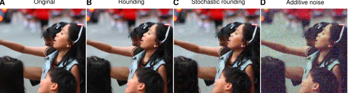
A Original B Rounding C Stochastic rounding D Additive noise
Figure 1: Effects of rounding and differentiable alternatives when used as replacements in JPEG compression. A: A crop of an image before compression (GoToVan, 2014). B: Blocking artefacts in JPEG are caused by rounding of DCT coefficients to the nearest integer. Since rounding is used at test time, a good approximation should produce similar artefacts. C: Stochastic rounding to the nearest integer similar to the binarization of Toderici et al. (2016a).D: Uniform additive noise (Ball´e et al., 2016).
forms of media. Notably, we achieve this performance using efficient neural network architectures which would allow near real-time decoding of large images even on low-powered consumer devices.
2 C
OMPRESSIVE AUTOENCODERSWe define a compressive autoencoder (CAE) to have three components: an encoderf, a decoderg, and a probabilistic modelQ,
f :RN →RM, g:RM →RN, Q:ZM →[0,1]. (1) The discrete probability distribution defined byQis used to assign a number of bits to represen- tations based on their frequencies, that is, for entropy coding. All three components may have parameters and our goal is to optimize the tradeoff between using a small number of bits and having small distortion,
−log2Q([f(x)])
| {z }
Number of bits
+β·d(x, g([f(x)]))
| {z }
Distortion
. (2)
Here,βcontrols the tradeoff, square brackets indicate quantization through rounding to the nearest integer, anddmeasures the distortion introduced by coding and decoding. The quantized output of the encoder is the code used to represent an image and is stored losslessly. The main source of information loss is the quantization (Appendix A.3). Additional information may be discarded by the encoder, and the decoder may not perfectly decode the available information, increasing distortion.
Unfortunately we cannot optimize Equation 2 directly using gradient-based techniques, asQand[·]
are non-differentiable. The following two sections propose a solution to deal with this problem.
2.1 QUANTIZATION AND DIFFERENTIABLE ALTERNATIVES
The derivative of the rounding function is zero everywhere except at integers, where it is undefined.
We propose to replace its derivative in the backward pass of backpropagation (Rumelhart et al., 1986) with the derivative of a smooth approximation,r, that is, effectively defining the derivative to be
d
dy[y] := d
dyr(y). (3)
Importantly, we do not fully replace the rounding function with a smooth approximation but only its derivative, which means that quantization is still performed as usual in the forward pass. If we replaced rounding with a smooth approximation completely, the decoder might learn to invert the
smooth approximation, thereby removing the information bottle neck that forces the network to compress information.
Empirically, we found the identity,r(y) = y, to work as well as more sophisticated choices. This makes this operation easy to implement, as we simply have to pass gradients without modification from the decoder to the encoder.
Note that the gradient with respect to the decoder’s parameters can be computed without resorting to approximations, assumingdis differentiable. In contrast to related approaches, our approach has the advantage that it does not change the gradients of the decoder, since the forward pass is kept the same.
In the following, we discuss alternative approaches proposed by other authors. Motivated by the- oretical links to dithering, Ball´e et al. (2016) proposed to replace quantization by additive uniform noise,
[f(x)]≈f(x) +u. (4)
Toderici et al. (2016a), on the other hand, used a stochastic form of binarization (Williams, 1992).
Generalizing this idea to integers, we define the following stochastic rounding operation:
{y} ≈ byc+ε, ε∈ {0,1}, P(ε= 1) =y− byc, (5) whereb·cis the floor operator. In the backward pass, the derivative is replaced with the derivative of the expectation,
d
dy{y}:= d
dyE[{y}] = d
dyy= 1. (6)
Figure 1 shows the effect of using these two alternatives as part of JPEG, whose encoder and decoder are based on a block-wise DCT transformation (Pennebaker & Mitchell, 1993). Note that the output is visibly different from the output produced with regular quantization by rounding and that the error signal sent to the autoencoder depends on these images. Whereas in Fig. 1B the error signal received by the decoder would be to remove blocking artefacts, the signal in Fig. 1D will be to remove high-frequency noise. We expect this difference to be less of a problem with simple metrics such as mean-squared error and to have a bigger impact when using more perceptually meaningful measures of distortion.
An alternative would be to use the latter approximations only for the gradient of the encoder but not for the gradients of the decoder. While this is possible, it comes at the cost of increased computa- tional and implementational complexity, since we would have to perform the forward and backward pass through the decoder twice: once using rounding, once using the approximation. With our approach the gradient of the decoder is correct even for a single forward and backward pass.
2.2 ENTROPY RATE ESTIMATION
SinceQis a discrete function, we cannot differentiate it with respect to its argument, which prevents us from computing a gradient for the encoder. To solve this problem, we use a continuous, differen- tiable approximation. We upper-bound the non-differentiable number of bits by first expressing the model’s distributionQin terms of a probability densityq,
Q(z) = Z
[−.5,.5[M
q(z+u)du. (7)
An upper bound is given by:
−log2Q(z) =−log2 Z
[−.5,.5[M
q(z+u)du≤ Z
[−.5,.5[M
−log2q(z+u)du, (8) where the second step follows from Jensen’s inequality (see also Theis et al., 2016). An unbiased estimate of the upper bound is obtained by samplingufrom the unit cube[−.5, .5[M. If we use a differentiable density, this estimate will be differentiable inzand therefore can be used to train the encoder.
2.3 VARIABLE BIT RATES
In practice we often want fine-gained control over the number of bits used. One way to achieve this is to train an autoencoder for different rate-distortion tradeoffs. But this would require us to train and store a potentially large number of models. To reduce these costs, we finetune a pre-trained autoencoder for different rates by introducing scale parameters1λ∈RM,
−log2q([f(x)◦λ] +u) +β·d(x, g([f(x)◦λ]/λ)). (9) Here,◦ indicates point-wise multiplication and division is also performed point-wise. To reduce the number of trainable scales, they may furthermore be shared across dimensions. Wheref andg are convolutional, for example, we share scale parameters across spatial dimensions but not across channels.
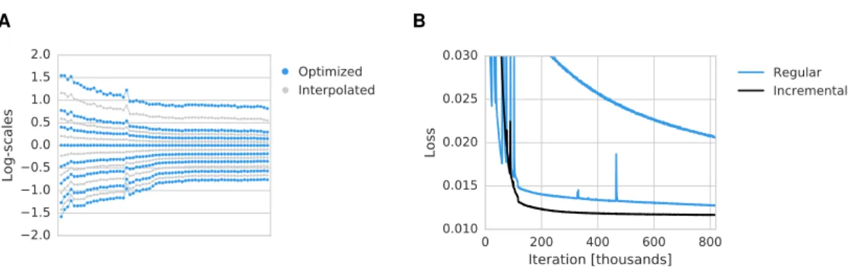
An example of learned scale parameters is shown in Figure 3A. For more fine-grained control over bit rates, the optimized scales can be interpolated.
2.4 RELATED WORK
Perhaps most closely related to our work is the work of Ball´e et al. (2016). The main differences lie in the way we deal with quantization (see Section 2.1) and entropy rate estimation. The transfor- mations used by Ball´e et al. (2016) consist of a single linear layer combined with a form of contrast gain control, while our framework relies on more standard deep convolutional neural networks.
Toderici et al. (2016a) proposed to use recurrent neural networks (RNNs) for compression. Instead of entropy coding as in our work, the network tries to minimize the distortion for a given number of bits. The image is encoded in an iterative manner, and decoding is performed in each step to be able to take into account residuals at the next iteration. An advantage of this design is that it allows for progressive coding of images. A disadvantage is that compression is much more time consum- ing than in our approach, as we use efficient convolutional neural networks and do not necessarily require decoding at the encoding stage.
Gregor et al. (2016) explored using variational autoencoders with recurrent encoders and decoders for compression of small images. This type of autoencoder is trained to maximize the lower bound of a log-likelihood, or equivalently to minimize
−Ep(y|x)
logq(y)q(x|y) p(y|x)
, (10)
wherep(y | x)plays the role of the encoder, andq(x | y)plays the role of the decoder. While Gregor et al. (2016) used a Gaussian distribution for the encoder, we can link their approach to the work of Ball´e et al. (2016) by assuming it to be uniform,p(y|x) =f(x) +u. If we also assume a Gaussian likelihood with fixed variance,q(x|y) =N(x|g(y), σ2I), the objective function can be written
Eu
−logq(f(x) +u) + 1
2σ2||x−g(f(x) +u)||2
+C. (11)
Here,Cis a constant which encompasses the negative entropy of the encoder and the normalization constant of the Gaussian likelihood. Note that this equation is identical to a rate-distortion trade-off withβ =σ−2/2and quantization replaced by additive uniform noise. However, not all distortions have an equivalent formulation as a variational autoencoder (Kingma & Welling, 2014). This only works ife−d(x,y) is normalizable in xand the normalization constant does not depend on y, or otherwiseCwill not be constant. An direct empirical comparison of our approach with variational autoencoders is provided in Appendix A.5.
Ollivier (2015) discusses variational autoencoders for lossless compression as well as connections to denoising autoencoders.
normalize mirror-pad conv conv conv conv sum conv conv sum conv
input round
GSM
128x5x5/2 64x5x5/2
128x3x3 128x3x3 128x3x3 128x3x3
96x5x5/2
subpix
512x3x3/2
conv conv
128x3x3 128x3x3
sum
conv conv
128x3x3 128x3x3
sum
subpix
subpix
256x3x3/2 12x3x3/2
clip
noise
output
code Model
Decoder Encoder
denormalize
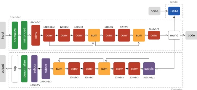
Figure 2: Illustration of the compressive autoencoder architecture used in this paper. Inspired by the work of Shi et al. (2016), most convolutions are performed in a downsampled space to speed up computation, and upsampling is performed using sub-pixel convolutions (convolutions followed by reshaping/reshuffling of the coefficients). To reduce clutter, only two residual blocks of the encoder and the decoder are shown. Convolutions followed by leaky rectifications are indicated by solid arrows, while transparent arrows indicate absence of additional nonlinearities. As a model for the distributions of quantized coefficients we use Gaussian scale mixtures. The notationC×K×K refers toK×Kconvolutions withCfilters. The number following the slash indicates stride in the case of convolutions, and upsampling factors in the case of sub-pixel convolutions.
3 E
XPERIMENTS3.1 ENCODER,DECODER,AND ENTROPY MODEL
We use common convolutional neural networks (LeCun et al., 1998) for the encoder and the decoder of the compressive autoencoder. Our architecture was inspired by the work of Shi et al. (2016), who demonstrated that super-resolution can be achieved much more efficiently by operating in the low- resolution space, that is, by convolving images and then upsampling instead of upsampling first and then convolving an image.
The first two layers of the encoder perform preprocessing, namely mirror padding and a fixed pixel- wise normalization. The mirror-padding was chosen such that the output of the encoder has the same spatial extent as an 8 times downsampled image. The normalization centers the distribution of each channel’s values and ensures it has approximately unit variance. Afterwards, the image is convolved and spatially downsampled while at the same time increasing the number of channels to 128. This is followed by three residual blocks (He et al., 2015), where each block consists of an additional two convolutional layers with 128 filters each. A final convolutional layer is applied and the coefficients downsampled again before quantization through rounding to the nearest integer.
The decoder mirrors the architecture of the encoder (Figure 9). Instead of mirror-padding andvalid convolutions, we use zero-padded convolutions. Upsampling is achieved through convolution fol- lowed by a reorganization of the coefficients. This reorganization turns a tensor with many channels into a tensor of the same dimensionality but with fewer channels and larger spatial extent (for de- tails, see Shi et al., 2016). A convolution and reorganization of coefficients together form asub-pixel convolution layer. Following three residual blocks, two sub-pixel convolution layers upsample the image to the resolution of the input. Finally, after denormalization, the pixel values are clipped to
1To ensure positivity, we use a different parametrization and optimize log-scales rather than scales.
2.01.5 1.00.5 0.00.5 1.01.5 2.0
Log-scales
Optimized Interpolated
A B
Figure 3:A: Scale parameters obtained by finetuning a compressive autoencoder (blue). More fine- grained control over bit rates can be achieved by interpolating scales (gray). Each dot corresponds to the scale parameter of one coefficient for a particular rate-distortion trade-off. The coefficients are ordered due to the incremental training procedure. B: Comparison of incremental training ver- sus non-incremental training. The learning rate was decreased after 116,000 iterations (bottom two lines). Non-incremental training is initially less stable and shows worse performance at later iter- ations. Using a small learning rate from the beginning stabilizes non-incremental training but is considerably slower (top line).
the range of 0 to 255. Similar to how we deal with gradients of the rounding function, we redefine the gradient of the clipping function to be 1 outside the clipped range. This ensures that the training signal is non-zero even when the decoded pixels are outside this range (Appendix A.1).
To model the distribution of coefficients and estimate the bit rate, we use independent Gaussian scale mixtures (GSMs),
log2q(z+u) =X
i,j,k
log2X
s
πksN(zkij+ukij; 0, σks2 ), (12) whereiandj iterate over spatial positions, andk iterates over channels of the coefficients for a single imagez. GSMs are well established as useful building blocks for modelling filter responses of natural images (e.g., Portilla et al., 2003). We used 6 scales in each GSM. Rather than using the more common parametrization above, we parametrized the GSM so that it can be easily used with gradient based methods, optimizing log-weights and log-precisions rather than weights and variances. We note that the leptokurtic nature of GSMs (Andrews & Mallows, 1974) means that the rate term encourages sparsity of coefficients.
All networks were implemented in Python using Theano (2016) and Lasagne (Dieleman et al., 2015).
For entropy encoding of the quantized coefficients, we first created Laplace-smoothed histogram estimates of the coefficient distributions across a training set. The estimated probabilities were then used with a publicly available BSD licensed implementation of a range coder2.
3.2 INCREMENTAL TRAINING
All models were trained usingAdam(Kingma & Ba, 2015) applied to batches of 32 images128×128 pixels in size. We found it beneficial to optimize coefficients in an incremental manner (Figure 3B).
This is done by introducing an additional binary maskm,
−log2q([f(x)]◦m+u) +β·d(x, g([f(x)]◦m)). (13) Initially, all but 2 entries of the mask are set to zero. Networks are trained until performance im- provements reach below a threshold, and then another coefficient is enabled by setting an entry of the binary mask to 1. After all coefficients have been enabled, the learning rate is reduced from an initial value of10−4 to10−5. Training was performed for up to106updates but usually reached good performance much earlier.
After a model has been trained for a fixed rate-distortion trade-off (β), we introduce and fine-tune scale parameters (Equation 9) for other values ofβ while keeping all other parameters fixed. Here
2https://github.com/kazuho/rangecoder/
JPEG (4:2:0, optimized) JP2 Toderici et al. (2016b)
CAE (ensemble)
0.0 0.5 1.0 1.5 2.0 2.5 3.0 Bit rate [bpp]
20 25 30 35 40 45
PSNR [dB]
0.0 0.5 1.0 1.5 2.0 2.5 3.0 Bit rate [bpp]
0.65 0.70 0.75 0.80 0.85 0.90 0.95 1.00
SSIM
0.0 0.5 1.0 1.5 2.0 2.5 3.0 Bit rate [bpp]
0.75 0.80 0.85 0.90 0.95 1.00
MS-SSIM
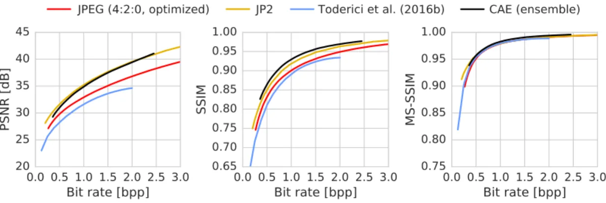
Figure 4: Comparison of different compression algorithms with respect to PSNR, SSIM, and MS- SSIM on the Kodak PhotoCD image dataset. We note that the blue line refers to the results of Toderici et al. (2016b) achievedwithoutentropy encoding.
we used an initial learning rate of10−3and continuously decreased it by a factor ofτκ/(τ+t)κ, wheretis the current number of updates performed,κ=.8, andτ= 1000. Scales were optimized for 10,000 iterations. For even more fine-grained control over the bit rates, we interpolated between scales optimized for nearby rate-distortion tradeoffs.
3.3 NATURAL IMAGES
We trained compressive autoencoders on 434 high quality images licensed under creative commons and obtained from flickr.com. The images were downsampled to below1536×1536pixels and stored as lossless PNGs to avoid compression artefacts. From these images, we extracted128× 128 crops to train the network. Mean squared error was used as a measure of distortion during training. Hyperparameters affecting network architecture and training were evaluated on a small set of held-out Flickr images. For testing, we use the commonly used Kodak PhotoCD dataset of 24 uncompressed768×512pixel images3.
We compared our method to JPEG (Wallace, 1991), JPEG 2000 (Skodras et al., 2001), and the RNN- based method of (Toderici et al., 2016b)4. Bits for header information were not counted towards the bit rate of JPEG and JPEG 2000. Among the different variants of JPEG, we found that optimized JPEG with 4:2:0 chroma sub-sampling generally worked best (Appendix A.2).
While fine-tuning a single compressive autoencoder for a wide range of bit rates worked well, opti- mizing all parameters of a network for a particular rate distortion trade-off still worked better. We here chose the compromise of combining autoencoders trained for low, medium or high bit rates (see Appendix A.4 for details).
For each image and bit rate, we choose the autoencoder producing the smallest distortion. This increases the time needed to compress an image, since an image has to be encoded and decoded multiple times. However, decoding an image is still as fast, since it only requires choosing and running one decoder network. A more efficient but potentially less performant solution would be to always choose the same autoencoder for a given rate-distortion tradeoff. We added 1 byte to the coding cost to encode which autoencoder of an ensemble is used.
Rate-distortion curves averaged over all test images are shown in Figure 4. We evaluated the differ- ent methods in terms of PSNR, SSIM (Wang et al., 2004a), and multiscale SSIM (MS-SSIM; Wang et al., 2004b). We used the implementation of van der Walt et al. (2014) for SSIM and the implemen- tation of Toderici et al. (2016b) for MS-SSIM. We find that in terms of PSNR, our method performs
3http://r0k.us/graphics/kodak/
4We used the code which was made available onhttps://github.com/tensorflow/models/
tree/2390974a/compression. We note that at the time of this writing, this implementation does not include entropy coding as in the paper of Toderici et al. (2016b).
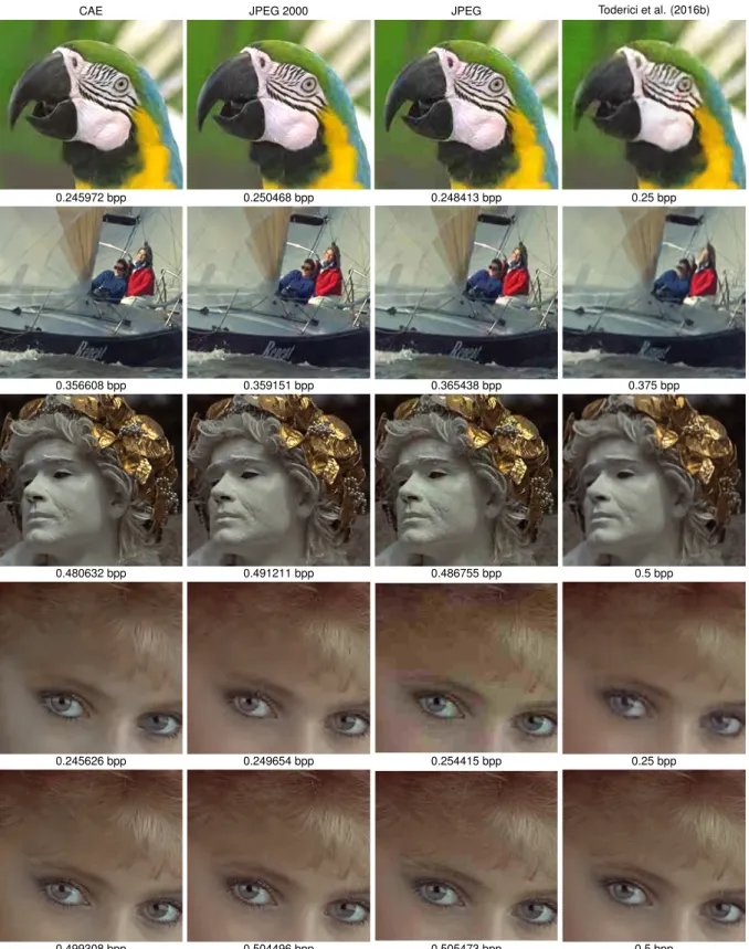
CAE JPEG 2000 JPEG Toderici et al. (2016b)
0.245972 bpp 0.250468 bpp 0.248413 bpp 0.25 bpp
0.356608 bpp 0.359151 bpp 0.365438 bpp 0.375 bpp
0.480632 bpp 0.491211 bpp 0.486755 bpp 0.5 bpp
0.245626 bpp 0.249654 bpp 0.254415 bpp 0.25 bpp
0.499308 bpp 0.504496 bpp 0.505473 bpp 0.5 bpp
Figure 5: Closeups of images produced by different compression algorithms at relatively low bit rates. The second row shows an example where our method performs well, producing sharper lines than and fewer artefacts than other methods. The fourth row shows an example where our method struggles, producing noticeable artefacts in the hair and discolouring the skin. At higher bit rates, these problems disappear and CAE reconstructions appear sharper than those of JPEG 2000 (fifth row). Complete images are provided in Appendix A.6.
0.25 0.375 0.5 Bit rate [bpp]
1 2 3 4 5
Mean Opinion Score± 95% CI
**
Lossless * Toderici et al., 2016b JPEG (4:2:0, optimized) JPEG2000 CAE
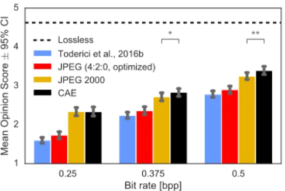
Figure 6: Results of a mean opinion score test.
similar to JPEG 2000 although slightly worse at low and medium bit rates and slightly better at high bit rates. In terms of SSIM, our method outperforms all other tested methods. MS-SSIM produces very similar scores for all methods, except at very low bit rates. However, we also find these re- sults to be highly image dependent. Results for individual images are provided as supplementary material5.
In Figure 5 we show crops of images compressed to low bit rates. In line with quantitative results, we find that JPEG 2000 reconstructions appear visually more similar to CAE reconstructions than those of other methods. However, artefacts produced by JPEG 2000 seem more noisy than CAE’s, which are smoother and sometimes appear G´abor-filter-like.
To quantify the subjective quality of compressed images, we ran amean opinion score(MOS) test.
While MOS tests have their limitations, they are a widely used standard for evaluating perceptual quality (Streijl et al., 2014). Our MOS test set included the 24 full-resolution uncompressed originals from the Kodak dataset, as well as the same images compressed using each of four algorithms at or near three different bit rates:0.25,0.372and0.5bits per pixel. Only the low-bit-rate CAE was included in this test.
For each image, we chose the CAE setting which produced the highest bit rate but did not exceed the target bit rate. The average bit rates of CAE compressed images were0.24479,0.36446, and 0.48596, respectively. We then chose the smallest quality factor for JPEG and JPEG 2000 for which the bit rate exceeded that of the CAE. The average bit rates for JPEG were0.25221,0.37339and 0.49534, for JPEG 20000.24631,0.36748and0.49373. For some images the bit rate of the CAE at the lowest setting was still higher than the target bit rate. These images were excluded from the final results, leaving 15, 21, and 23 images, respectively.
The perceptual quality of the resulting273images was rated byn= 24non-expert evaluators. One evaluator did not finish the experiment, so her data was discarded. The images were presented to each individual in a random order. The evaluators gave a discrete opinion score for each image from a scale between1(bad) to5(excellent). Before the rating began, subjects were presented an uncompressed calibration image of the same dimensions as the test images (but not from the Kodak dataset). They were then shown four versions of the calibration image using the worst quality setting of all four compression methods, and given the instruction “These are examples of compressed images. These are some of the worst quality examples.”
Figure 6 shows average MOS results for each algorithm at each bit rate. 95% confidence intervals were computed via bootstrapping. We found that CAE and JPEG 2000 achieved higher MOS than JPEG or the method of Toderici et al. (2016b) at all bit rates we tested. We also found that CAE significantly outperformed JPEG 2000 at0.375bpp(p <0.05) and0.5bpp(p <0.001).
5https://figshare.com/articles/supplementary_zip/4210152
4 D
ISCUSSIONWe have introduced a simple but effective way of dealing with non-differentiability in training au- toencoders for lossy compression. Together with an incremental training strategy, this enabled us to achieve better performance than JPEG 2000 in terms of SSIM and MOS scores. Notably, this perfor- mance was achieved using an efficient convolutional architecture, combined with simple rounding- based quantization and a simple entropy coding scheme. Existing codecs often benefit from hard- ware support, allowing them to run at low energy costs. However, hardware chips optimized for convolutional neural networks are likely to be widely available soon, given that these networks are now key to good performance in so many applications.
While other trained algorithms have been shown to provide similar results as JPEG 2000 (e.g.
van den Oord & Schrauwen, 2014), to our knowledge this is the first time that an end-to-end trained architecture has been demonstrated to achieve this level of performance on high-resolution images.
Anend-to-endtrained autoencoder has the advantage that it can be optimized for arbitrary metrics.
Unfortunately, research on perceptually relevant metrics suitable for optimization is still in its in- fancy (e.g., Dosovitskiy & Brox, 2016; Ball´e et al., 2016). While perceptual metrics exist which correlate well with human perception for certain types of distortions (e.g., Wang et al., 2004a; La- parra et al., 2016), developing a perceptual metric which can be optimized is a more challenging task, since this requires the metric to behave well for a much larger variety of distortions and image pairs.
In future work, we would like to explore the optimization of compressive autoencoders for different metrics. A promising direction was presented by Bruna et al. (2016), who achieved interesting super- resolution results using metrics based on neural networks trained for image classification. Gatys et al. (2016) used similar representations to achieve a breakthrough in perceptually meaningful style transfer. An alternative to perceptual metrics may be to use generative adversarial networks (GANs;
Goodfellow et al., 2014). Building on the work of Bruna et al. (2016) and Dosovitskiy & Brox (2016), Ledig et al. (2016) recently demonstrated impressive super-resolution results by combining GANs with feature-based metrics.
ACKNOWLEDGMENTS
We would like to thank Zehan Wang, Aly Tejani, Cl´ement Farabet, and Luke Alonso for helpful feedback on the manuscript.
R
EFERENCESD. F. Andrews and C. L. Mallows. Scale mixtures of normal distributions. Journal of the Royal Statistical Society, Series B, 36(1):99–102, 1974.
J. Ball´e, V. Laparra, and E. P. Simoncelli. End-to-end optimization of nonlinear transform codes for perceptual quality. InPicture Coding Symposium, 2016.
J. Bruna, P. Sprechmann, and Y. LeCun. Super-resolution with deep convolutional sufficient statis- tics. InThe International Conference on Learning Representations, 2016.
S. Dieleman, J. Schluter, C. Raffel, E. Olson, S. K. Sonderby, D. Nouri, D. Maturana, M. Thoma, E. Battenberg, J. Kelly, J. De Fauw, M. Heilman, D. Moitinho de Almeida, B. McFee, H. Weide- man, G. Takacs, P. de Rivaz, J. Crall, G. Sanders, K. Rasul, C. Liu, G. French, and J. Degrave.
Lasagne: First release, 2015. URLhttp://dx.doi.org/10.5281/zenodo.27878.
A. Dosovitskiy and T. Brox. Generating images with perceptual similarity metrics based on deep networks, 2016. arXiv:1602.02644.
L. A. Gatys, A. S. Ecker, and M. Bethge. Image style transfer using convolutional neural networks.
InProceedings of the IEEE Conference on Computer Vision and Pattern Recognition, 2016.
I. Goodfellow, J. Pouget-Abadie, M. Mirza, B. Xu, D. Warde-Farley, S. Ozair, A. Courville, , and Y. Bengio. Generative adversarial nets. InAdvances in Neural Information Processing Systems 27, 2014.
GoToVan. Canada day parade, 2014. URLhttps://www.flickr.com/photos/gotovan/
14579921203.
K. Gregor, I. Danihelka, A. Graves, and D. Wierstra. Towards conceptual compression, 2016.
arXiv:1601.06759.
K. He, X. Zhang, S. Ren, and J. Sun. Deep residual learning for image recognition, 2015.
arXiv:1512.03385.
D. Kingma and M. Welling. Auto-encoding variational bayes. In International Conference on Learning Representations, 2014.
D. P. Kingma and J. Ba. Adam: A Method for Stochastic Optimization. In The International Conference on Learning Representations, 2015.
V. Laparra, J. Ball´e, and E. P. Simoncelli. Perceptual image quality assessment using a normalized Laplacian pyramid. InSPIE, Conf. on Human Vision and Electronic Imaging, XXI, 2016.
Y. LeCun, L. Bottou, Y. Bengio, and P. Haffner. Gradient-based learning applied to document recognition. 86(11), 1998.
C. Ledig, L. Theis, F. Huszar, J. Caballero, A. Aitken, A. Tejani, J. Totz, Z. Wang, and W. Shi.
Photo-Realistic Single Image Super-Resolution Using a Generative Adversarial Network, 2016.
arXiv:1609.04802.
Y. Ollivier. Auto-encoders: reconstruction versus compression, 2015. 1403.7752.
W. B. Pennebaker and J. L. Mitchell. JPEG still image data compression standard. Springer, 3rd edition, 1993.
J. Portilla, V. Strela, M. J. Wainwright, and E. P. Simoncelli. Image denoising using scale mixtures of gaussians in the wavelet domain.IEE Trans. Image Process., 12(11):1338–1351, 2003.
D. E. Rumelhart, G. E. Hinton, and R. J. Williams. Learning representations by back-propagating errors.Nature, 323(6088):533–536, 1986.
W. Shi, J. Caballero, F. Huszar, J. Totz, A. Aitken, R. Bishop, D. Rueckert, and Z. Wang. Real-time single image and video super-resolution using an efficient sub-pixel convolutional neural network.
InIEEE Conf. on Computer Vision and Pattern Recognition, 2016.
A. Skodras, C. Christopoulos, and T. Ebrahimi. The JPEG 2000 still image compression standard.
Signal Processing Magazine, 18(5):36–58, 2001.
R. C. Streijl, S. Winkler, and D. S. Hands. Mean opinion score (MOS) revisited: methods and applications, limitations and alternatives.Multimedia Systems, pp. 1–15, 2014.
D. Del Testa and M. Rossi. Lightweight Lossy Compression of Biometric Patterns via Denoising Autoencoders.IEEE Signal Processing Letters, 22(12), 2016.
Theano Development Team. Theano: A Python framework for fast computation of mathematical expressions, 2016. arXiv:1605.02688.
L. Theis and M. Bethge. Generative Image Modeling Using Spatial LSTMs. InAdvances in Neural Information Processing Systems 28, 2015.
L. Theis, A. van den Oord, and M. Bethge. A note on the evaluation of generative models. InThe International Conference on Learning Representations, 2016.
G. Toderici, S. M. O’Malley, S. J. Hwang, D. Vincent, D. Minnen, S. Baluja, M. Covell, and R. Suk- thankar. Variable rate image compression with recurrent neural networks. InThe International Conference on Learning Representations, 2016a.
G. Toderici, D. Vincent, N. Johnston, S. J. Hwang, D. Minnen, J. Shor, and M. Covell. Full resolution image compression with recurrent neural networks, 2016b. arXiv:1608.05148v1.
A. van den Oord and B. Schrauwen. The student-t mixture as a natural image patch prior with application to image compression. Journal of Machine Learning Research, 15(1):2061–2086, 2014.
A. van den Oord, N. Kalchbrenner, and K. Kavukcuoglu. Pixel recurrent neural networks. In Proceedings of the 33rd International Conference on Machine Learning, 2016a.
A. van den Oord, N. Kalchbrenner, O. Vinyals, L. Espeholt, A. Graves, and K. Kavukcuoglu. Con- ditional Image Generation with PixelCNN Decoders, 2016b. arXiv:1606.05328v2.
S. van der Walt, J. L. Sch¨onberger, J. Nunez-Iglesias, F. Boulogne, J. D. Warner, N. Yager, E. Gouil- lart, and T. Yu. scikit-image: image processing in Python.PeerJ, 2, 2014.
G. K. Wallace. The JPEG still picture compression standard. Communications of the ACM, 34(4):
30–44, 1991.
Z. Wang, A. C. Bovik, H. R. Sheikh, and E. P. Simoncelli. Image quality assessment: from error visibility to structural similarity.IEEE Transactions on Image Processing, 13(4):600–612, 2004a.
Z. Wang, E. P. Simoncelli, and A. C. Bovik. Multiscale structural similarity for image quality assessment. InConference Record of the Thirty-Seventh Asilomar Conference on Signals, Systems and Computers, volume 2, pp. 1398–1402, 2004b.
R. J. Williams. Simple statistical gradient-following algorithms for connectionist reinforcement learning.Machine Learning, 8(3-4):229–256, 1992.
A A
PPENDIXA.1 GRADIENT OF CLIPPING
We redefine the gradient of the clipping operation to be constant, d
dˆxclip0,255(ˆx) := 1. (14)
Consider how this affects the gradients of a squared loss, d
dˆx(clip0,255(ˆx)−x)2= 2(clip0,255(ˆx)−x) d
dˆxclip0,255(ˆx). (15) Assume thatxˆis larger than 255. Without redefinition of the derivative, the error signal will be 0 and not helpful. Without any clipping, the error signal will depend on the value ofx, even thoughˆ any value above 255 will have the same effect on the loss at test time. On the other hand, using clipping but a different signal in the backward pass is intuitive, as it yields an error signal which is proportional to the error that would also be incurred at test time.
A.2 DIFFERENT MODES OFJPEG
We compared optimized and non-optimized JPEG with (4:2:0) and without (4:4:4) chroma sub- sampling. Optimized JPEG computes a Huffman table specific to a given image, while unoptimized JPEG uses a predefined Huffman table. We did not count bits allocated to the header of the file format, but for optimized JPEG we counted the bits required to store the Huffman table. We found that on average, chroma-subsampled and optimized JPEG performed better on the Kodak dataset (Figure 7).
A.3 COMPRESSION VS DIMENSIONALITY REDUCTION
Since a single real number can carry as much information as a high-dimensional entity, dimensional- ity reduction alone does not amount to compression. However, if we constrain the architecture of the encoder, it may be forced to discard certain information. To better understand how much information is lost due to dimensionality reduction and how much information is lost due to quantization, Fig- ure 8 shows reconstructions produced by a compressive autoencoder with and without quantization.
The effect of dimensionality reduction is minimal compared to the effect of quantization.
JPEG (4:2:0)
JPEG (4:4:4) JPEG (4:2:0, optimized)
JPEG (4:4:4, optimized)
0.0 0.5 1.0 1.5 2.0 2.5 3.0 Bit-rate [bit/px]
20 25 30 35 40 45
PSNR [dB]
0.0 0.5 1.0 1.5 2.0 2.5 3.0 Bit-rate [bit/px]
0.65 0.70 0.75 0.80 0.85 0.90 0.95 1.00
SSIM
0.0 0.5 1.0 1.5 2.0 2.5 3.0 Bit-rate [bit/px]
0.75 0.80 0.85 0.90 0.95 1.00
MS-SSIM
Figure 7: A comparison of different JPEG modes on the Kodak PhotoCD image dataset. Optimized Huffman tables perform better than default Huffman tables.
A Original B Dim. reduction C Rounding
Figure 8: To disentangle the effects of quantization and dimensionality reduction, we reconstructed images with quantization disabled. A: The original uncompressed image. B: A reconstruction gen- erated by a compressive autoencoder, but with the rounding operation removed. The dimensionality of the encoder’s output is3×smaller than the input. C: A reconstruction generated by the same compressive autoencoder. While the effects of dimensionality reduction are almost imperceptible, quantization introduces visible artefacts.
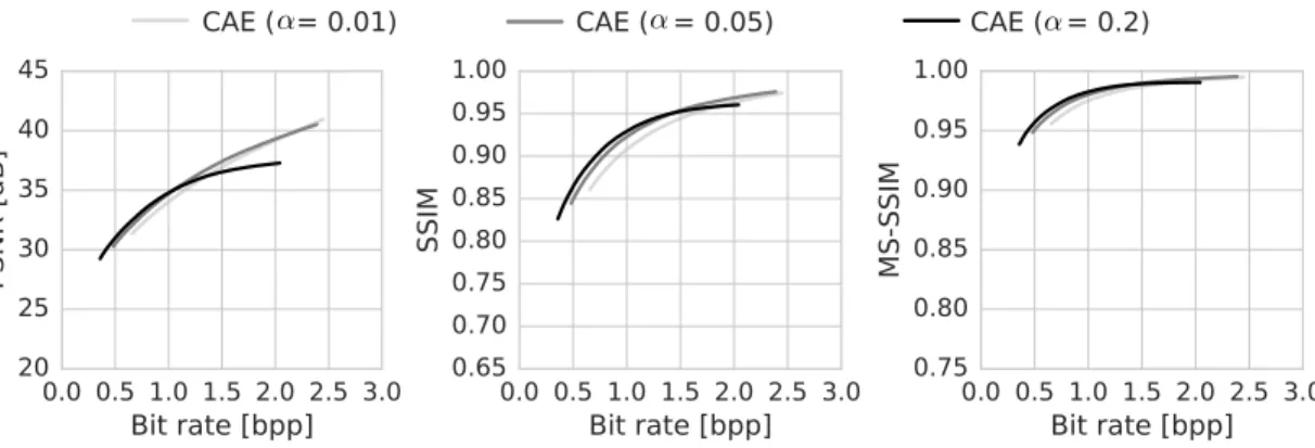
A.4 ENSEMBLE
CAE (
↵= 0.01)
CAE (
↵= 0.05)
CAE (
↵= 0.2)
0.0 0.5 1.0 1.5 2.0 2.5 3.0 Bit rate [bpp]
20 25 30 35 40 45
PSNR [dB]
0.0 0.5 1.0 1.5 2.0 2.5 3.0 Bit rate [bpp]
0.65 0.70 0.75 0.80 0.85 0.90 0.95 1.00
SSIM
0.0 0.5 1.0 1.5 2.0 2.5 3.0 Bit rate [bpp]
0.75 0.80 0.85 0.90 0.95 1.00
MS-SSIM
Figure 9: Comparison of CAEs optimized for low, medium, or high bit rates.
To bring the parameter controlling the rate-distortion trade-off into a more intuitive range, we rescaled the distortion term and expressed the objective as follows:
−α
N lnq([f(x)◦λ] +u) + 1−α
1000·M · ||x−g([f(x)◦λ]/λ)||2. (16) Here,N is the number of coefficients produced by the encoder andM is the dimensionality ofx (i.e., 3 times the number of pixels).
The high-bit-rate CAE was trained with α = 0.01and 96 output channels, the medium-bit-rate CAE was trained withα= 0.05and 96 output channels, and the low-bit-rate CAE was trained with α= 0.2and 64 output channels.
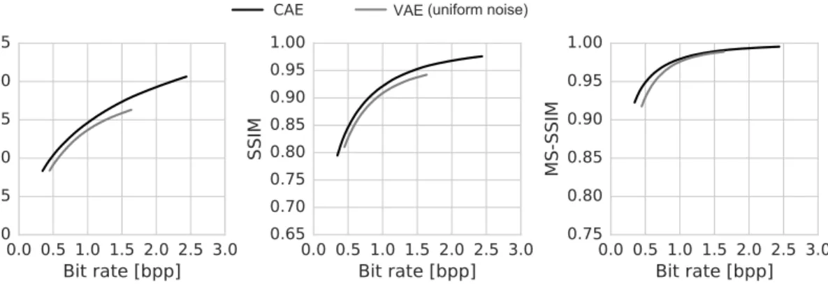
A.5 COMPARISON WITHVAE
VAE(uniform noise)
0.0 0.5 1.0 1.5 2.0 2.5 3.0 Bit rate [bpp]
20 25 30 35 40 45
PSNR [dB]
0.0 0.5 1.0 1.5 2.0 2.5 3.0 Bit rate [bpp]
0.65 0.70 0.75 0.80 0.85 0.90 0.95 1.00
SSIM
0.0 0.5 1.0 1.5 2.0 2.5 3.0 Bit rate [bpp]
0.75 0.80 0.85 0.90 0.95 1.00
MS-SSIM
Figure 10: An alternative to our approach is to replace the rounding function with additive uni- form noise during training (Ball´e et al., 2016). Using mean-squared error for measuring distortion, optimizing rate-distortion this way is equivalent to training a variational autoencoder (Kingma &
Welling, 2014) with a Gaussian likelihood and uniform encoder (Section 2.4). Using the same train- ing proecedure autoencoder architecture for both approaches (here trained for high bit-rates), we find that additive noise performs worse than redefining derivatives as in our approach. Rounding-based quantization is used at test time in both approaches.
A.6 COMPLETE IMAGES
Below we show complete images corresponding to the crops in Figure 5. For each image, we show the original image (top left), reconstructions using CAE (top right), reconstructions using JPEG 2000 (bottom left) and reconstructions using the method of (Toderici et al., 2016b) (bottom right).
The images are best viewed on a monitor screen.