Potential Output, the Natural Rate of Unemployment, and the Phillips Curve in a Multivariate Structural Time Series Framework

(1)

IHS Economics Series Working Paper 33

June 1996

Potential Output, the Natural Rate of Unemployment, and the Phillips Curve in a Multivariate Structural Time Series Framework

Franz Hahn

Gerhard Rünstler

(2)

Impressum Author(s):

Franz Hahn, Gerhard Rünstler Title:

Potential Output, the Natural Rate of Unemployment, and the Phillips Curve in a Multivariate Structural Time Series Framework

ISSN: Unspecified

1996 Institut für Höhere Studien - Institute for Advanced Studies (IHS) Josefstädter Straße 39, A-1080 Wien

E-Mail: o ce@ihs.ac.atﬃ Web: ww w .ihs.ac. a t

All IHS Working Papers are available online: http://irihs. ihs. ac.at/view/ihs_series/

This paper is available for download without charge at: https://irihs.ihs.ac.at/id/eprint/913/

(3)

Institut für Höhere Studien (IHS), Wien Institute for Advanced Studies, Vienna

Reihe Ökonomie / Economics Series No. 33

Potential Output, the Natural Rate of

Unemployment, and the Phillips Curve in a Multivariate Structural Time Series

Framework

Franz Hahn, Gerhard Rünstler

(4)

Potential Output, the Natural Rate of

Unemployment, and the Phillips Curve in a Multivariate Structural Time Series

Framework

Franz Hahn, Gerhard Rünstler

Reihe Ökonomie / Economics Series No. 33

June 1996

Franz Hahn

Austrian Institute for Economic Research P.O. Box 91

A-1103 Vienna, Austria Phone: ++43-1-798-2601/255 Fax: ++43-1-798-9386 e-mail: hahn@wsr.ac.at Gerhard Rünstler Department of Economics Institute for Advanced Studies Stumpergasse 56

A-1060 Vienna, Austria Phone: ++43-1-59991-151 Fax: + ++43-1-59991-163 e-mail: ruenstle@ihssv.wsr.ac.at

Institut für Höhere Studien (IHS), Wien

Institute for Advanced Studies, Vienna

(5)

The Institute for Advanced Studies in Vienna is an independent center of postgraduate training and research in the social sciences. The Economics Series presents research done at the Economics Department of the Institute for Advanced Studies. Department members, guests, visitors, and other researchers are invited to contribute and to submit manuscripts to the editors. All papers are subjected to an internal refereeing process.

Editorial Main Editor:

Robert M. Kunst (Econometrics) Associate Editors:

Christian Helmenstein (Macroeconomics) Arno Riedl (Microeconomics)

(6)

Abstract

We propose a bivariate structural time series framework to decompose GDP and the unemployment rate into their trend, cyclical, and irregular components. We implement Okun’s law by a generalised version of the common cycles restriction allowing for a phase shift between the two cycles and add a price-wage block to the system. We estimate by maximum likelihood Phillips curve-type equations, where the particular cycles enter the wage and price equations in levels though the trends are modelled as non-stationary stochastic processes. The extended models provide an improved estimate of the current cyclical position, compared to univariate estimates and the HP filter.

Keywords

Structural time series model, trends and cycles, Pillips curve

JEL-Classifications

C22, E30

(7)

Comments

This work is based on a study performed for the Austrian Ministry of Finance; The authors would like to thank to R. Kunst, K. Pichelmann, G. Thury, and M. Wüger for valuable comments and suggestions.

(8)

I H S — Hahn, Rünstler / Potential Output, the Natural Rate of Unemployment — 1

1. Introduction

The decomposition of macroeconomic time series into their long-run trend and cyclical components has become a matter of lasting concern. Among many uses one important application is the assessment of the fiscal and monetary policy stance from the cyclical position of GDP and the unemployment rate. It has recently gained renewed attention for the goal of cyclical adjustment of government budget balances in the course of the consolidation efforts of EU member states (Giorno et. al., 1995; European Commission, 1995b, Barrell et.

al., 1994). The traditional theoretical foundations for the dichotomy between trend and cyclical components lie in the neo-classical synthesis and aggregate demand-supply models, respectively. The long-run trend in GDP is determined by a production function, while cyclical deviations occur due to price- and wage rigidities translating demand shocks into output fluctuations. Price and wage behaviour is traditionally described by Tobin’s wage-price mechanism giving rise to the well-known unemployment-inflation trade-off. At potential output and the natural rate of unemployment, respectively, there occurs no inflationary pressure from the labour market.

There are numerous methods for the extraction of trend and cyclical components (see, e.g.

Canova, 1993). Among the currently most widely used are non-parametric smoothing techniques, i.e., the Hodrick-Prescott (HP) filter (Hodrick and Prescott, 1980), the Beveridge- Nelson-decomposition (e.g., King et. al., 1991; Evans and Reichlin, 1994; Karras, 1994;

Sefton, 1995), and the production function approach (e.g., Torres and Martin, 1990; Giorno et. al., 1995). These methods differ widely in the utilisation of economically motivated restrictions as outlined above. While smoothing techniques are atheoretical by their nature, the production function approach makes explicit use of the close co-movement of GDP and unemployment cycles and the property of inflation neutrality of potential GDP. Potential output is defined as the outcome of a production function, i.e., PO = q^PO f(K, L^PO), where the factor inputs and total factor productivity are at their potential levels. Total factor productivity at potential output q^PO is found by smoothing techniques, while potential employment L^PO is calculated from the smoothed labour supply and an estimate of the unemployment rate that is consistent with non-accelerating inflation (e.g., Layard, Nickell and Jackman, 1991). The third approach, the multivariate Beveridge-Nelson-decomposition, based on vector autoregressions, uses the information contained in the co-movement of GDP with various cyclical indicators and/or common trend restrictions in order to decompose GDP into a random walk and a stationary component. However, there are clear limitations to imposing restrictions related to the above cyclical relationships. In particular, as the VARs are specified in first differences, Phillips curve type relationships relating prices and wages to cycles in levels cannot be modelled explicitly.

(9)

2 — Hahn, Rünstlerr / Potential Output, the Natural Rate of Unemployment — I H S

From an econometric viewpoint, smoothing techniques and the production function approach suffer from several shortcomings. As concerns the HP filter, it has been criticised for various deficiencies (e.g., King and Rebelo, 1993), the most important being the arbitrariness of the smoothing parameter and its tendency to produce spurious cycles (Harvey and Jäger, 1992;

Boone and Hall, 1995). Since the HP filter is also used in the production function approach (Giorno et. al., 1995) for smoothing labour supply and total factor productivity, its shortcomings also apply to a somewhat less extent to the latter.¹ Moreover, as a general feature, smoothing techniques based on two-sided symmetric moving averages of past and future observations give rise to a substantial so-called end-point bias, i.e., biased estimates at the end of the sample (Barrell et. al., 1994). For policy purposes, however, the estimate of the current cyclical position is certainly the most important outcome of the whole exercise.

The present paper proposes an approach that allows for explicitly modelling cyclical relationships in levels and estimation within a maximum likelihood framework. It is based on a multivariate extension of structural time series (STS) models, advocated in a series of papers by Harvey (Harvey, 1985, 1989; Harvey et. al. 1986; Harvey and Koopman, 1992;

Harvey and Jäger, 1993). STS models are designed to decompose a time series into several unobserved components, i.e., a non-stationary trend, a cycle, and an irregular term. The particular components are specified as separate parametric stochastic processes. This specific feature allows for imposing restrictions on the particular components. We construct a bivariate STS model for GDP and the unemployment rate and impose a close co-movement of the two cycles. We also add wage and price equations to the system with the cycles and provide a full maximum likelihood estimate of a Phillips curve in its traditional form, where prices and wages are related to the cyclical components in levels though the trends follow non-stationary processes. The wage-price block allows for a misspecification test for the property of inflation neutrality of the particular trends, as extracted by the model. After an outline of our approach we present results for Austrian quarterly data. We will compare estimates from the HP filter and univariate STS models with the multivariate approach.

1 Röger (1994) has pointed out that the application of the HP-Filter to all factor inputs is equivalent to its application to GDP itself. Moreover, work by the European Commission (1995a) indicates that traditional NAIRU estimates based on wage and price equations exhibit a high degree of uncertainty. with their confidence bounds up to ± 3 percentage points. Thus, in fact, the NAIRU estimates are often subject to judgemental revision.

(10)

2. Structural Time Series (STS) Models

The following model has been proposed by Harvey (1985) for the decomposition of a macroeconomic time series y into a non-stationary trend y^tr, a stationary cycle ϕ, and an irregular component ν.

(1) yt = yttr + ϕt + νt

The trend follows a so-called local linear trend, that is a random walk with stochastic drift µt

which, in turn, again is specified as random walk, i.e.,

(2) ∆yttr = µ_t-1 + ηt(1)

∆µt = ηt(2)

where ηt(1) and ηt(2) are white noise. This is an ARIMA(0,2,2) process. If σ12 = var(ηt(1)) = 0 the model reduces to a random walk with drift. If σ12 = 0, but σ22 = var(ηt(2)) > 0, the trend is still a process integrated of order 2, i.e., ∆² yttr = ηt(2). Such a trend tends to be relatively smooth compared to a random walk, with a more or less slowly changing slope.

The cyclical component ϕt is specified as a so-called stochastic cycle,

(3)  ϕ_t  =

ρ

 cos

λ

^sin

λ

  ϕ_t-1 + η_t⁽^ϕ⁾

 ϕ_t*   -sin

λ

^cos

λ

  ϕ_t-1* η_t^(ϕ)* , with |

ρ

^{| < 1,}

which is derived from a dampened cosine wave of fixed length λ, subject to shocks η_t^(ϕ) and η_t⁽^ϕ⁾*. In its ARIMA form it turns out to be a stationary ARMA(2,1) process, whose AR- polynomial is restricted to have two conjugate complex roots thereby generating a cyclical impulse response to both innovations (Harvey, 1989). The whole model can be written in state-space form with the state vector ααt = (yttr, µt, ϕt, ϕt*)’, and the vector of innovations ηηt = (ηt(1), ηt(2), ηt(ϕ), ηt(ϕ)*)’. For identification, the restrictions E νtηt(i) = 0 and E ηt(i)ηt(j)

= 0, for i≠j, have to be imposed, thus giving a diagonal variance-covariance matrix cov(ηηt). Also, the restriction σϕ2 = var(ηt(ϕ)) = var(ηt(ϕ)*) is usually imposed. Finally, the set of hyperparameters (

ρ

,

λ

, σν2, cov(ηηt)) may be estimated by maximum likelihood (ML) using the Kalman filter.

Once the hyperparameters have been estimated, the Kalman filter gives the optimal filtered estimates ααt|t of the state vector ααt at time t, given past and current observations (y1,...,y_t).

The subsequent application of a smoothing algorithm provides optimal smoothed estimates ααt|T for ααt given all available observations (y1,..., yT).

It is also noteworthy that STS models encompass the HP filter. The HP filter can be characterised as the optimal estimator of the STS model y_t = y_t^tr + νt, composed of a smooth trend (σ12 = 0) and an irregular component, but without a cycle. The smoothing parameter τHP

(11)

is given as the ratio of the variances of the irregular component and the change in the slope, i.e., τHP = σν2/σ22. The HP filter estimate of the cycle is then nothing but the smoothed irregular component with the value of τHP imposed rather than estimated (Harvey and Jäger, 1993).

2.1. Possible Restrictions on Cyclical Components

The extension of the above univariate STS model to the multivariate case is straightforward.

The simplest case, in the context of a bivariate model for two series y_t and ur_t,

(4) y_t = y_t^tr + ϕt(y) + νt (y)

ur_t = ur_t^tr + ϕt(ur) + νt (ur)

would be the simultaneous estimation of the two equations, possibly allowing for correlations between corresponding innovations η_t^(y,i) and η_t^(ur,i). The bivariate model (4) can be easily stacked in one single state-space form. The literature so far suggests two ways to establish a link among different cyclical components. In the so-called similar cycles (SC) model the cycles ϕ_t^(y) and ϕ_t^(ur) are independent of each other with the only restriction that the cycle lengths are equal, i.e., λy = λur. The common cycles (CC) model incorporates only one cycle ϕ_t at which the particular series participate with different scaling parameters 1 and θ, i.e., ϕt(ur)

= θ ϕt(y). Both restrictions seem not entirely satisfactory for the purpose of modelling the business cycle. In the SC model there is no direct link between the cycles and nothing prevents them from moving rather independently with, for instance, very different turning points. On the other hand, the CC model obviously is incapable of modelling possible leads or lags between different cycles. However, it is well-known that the unemployment cycle generally follows the output one with a time lag of up to several quarters. We therefore use a generalisation of the common cycles model (GCC), proposed by Rünstler (1996), where the cyclical component of urt is also linked to ϕt* from equation (3).

(5) yt = yttr + ϕt + νt(y) t

urt = urttr + (θ ϕt + θ*ϕt*) + νt(ur)

This simple generalisation has the appealing interpretation that (θϕ_t + θ*ϕ_t*) follows (or leads) the original cycle ϕ_t with a constant phase shift ω = λ^-1 arctan(θ*/θ). Its variance relative to the variance of ϕ_t is given by the scaling factor ϑ² = θ² + θ*². More precisely, any linear combination (θϕ_t + θ*ϕ_t*) of ϕ_t and ϕ_t* follows the same autocorrelation function

corr (θϕ_t + θ*ϕ_t*, θϕ_t-s + θ*ϕ_t-s*) = ρ^s cos (λs),

independent of θ and θ*, while the crosscorrelations between ϕ_t and (θϕ_t-s + θ*ϕ_t-s*) are given by

(12)

corr (ϕ_t, θϕ_t-s + θ*ϕ_t-s*) = ρ^s (θ ² + θ* ²)^-1/2 (θ cos(λs) + θ* sin (λs)).

= ρ^s cos(λ(s - ω)).

Obviously, the crosscorrelation function reaches its local extremes at s - ω = k π/2 with the global maximum at s = ω. Thus ω gives the phase shift of (θϕ_t + θ*ϕ_t*) with respect to ϕ_t. Also, as there is a pair of shocks η_t⁽^ϕ⁾ and η_t⁽^ϕ⁾*, the relationship between the two cycles is not deterministic. The bivariate GCC model might be regarded as a restricted bivariate AR(1) process with conjugate complex roots. This can be seen from the fact that the two cyclical components, ϕt(y) andϕt(ur), are linear transformations of ϕ_t and ϕ_t*.

Tests of the SC and GCC restrictions can be conducted using likelihood ratio (LR) tests. The test of the SC restriction, H0: λy = λur, is straightforward with the LR-statistics following a χ₁² distribution. Testing for the GCC restriction amounts to testing for the presence of a further stochastic cycle (3), ψt, in the GCC model. For identification reasons it is sufficient to add ψt

to one of either equations.

(6) yt = yttr + ϕt + νt(y)

urt = urttr + (θ ϕt + θ*ϕt*) + ψt

As Harvey (1989) points out, the test for the presence of the cycle ψt is equivalent to imposing the restriction H₀: ρψ = 0 on the corresponding dampening factor. In this case ψt

becomes white noise. In general, the LR-test of H₀ is not feasible due to the complication that λψ is no longer identified under H0. In the context of testing the GCC restriction, however, λψ

might be set equal to the cycle length λ of ϕt. Also, since under H₀ ψt is not distinguishable from the irregular component ν_t^(ur), σ_ψ² is also unidentified. Thus, νt(ur) must be removed from the unrestricted model. Under H₀: ρψ = 0 equation (6) then nevertheless reduces to equation (5).²

2.2. Price and Wage Equations

Non-stationary trends, as extracted by the above methods, do not account for inflation neutrality. Since the technology for calculating the NAIRU requires an estimated relation between inflation and the unemployment rate, it is inextricably linked to dynamic Phillips curve equations for price and wage changes. We therefore add standard price and wage equations to the bivariate models, that is, we aim at estimating a model of the general structure

(7) y_t = y_t^tr + ϕ_t^(y) + ν_t^(y)

2 For the univariate model, Harvey (1989, p. 251) proposes an LM test for the presence of a further cyclical component in the series based on a regression of the periodigram on the elements of the spectral generating function.

(13)

ur_t = ur

t

tr + ϕ_t^(ur) + ν_t^(ur)

∆pt = a₁(L) ∆wt-1 + a₂(L) ∆pt-1 + a₃(L) ∆qt-1 + a₄ (s_t-k - µ) + β1 ϕ_t-l^(y)+ ε_t^(p)

∆wt = b₁(L) ∆wt-1 + b₂(L) ∆pt-1 + b₃(L) ∆qt-1 - b₄ (s_t-k - µ) - β2 ϕ_t-l^(ur)+ ε_t^(w),

where either of the above restrictions on cyclical co-movements might be imposed. The general specification of the price and wage equations follows Franz and Gordon (1994) and Pichelmann (1993). p, w, and q denote prices, wages, and labour productivity (in logs). The labour share of income s_t-k acts as an error-correction term accounting for the stationary long-run relationship between real wages and labour productivity. The constant µ enters the error-correction term thereby implying the absence of a linear trend component in prices and wages.

Estimates of the NAIRU, as used in the production function approach, combine the wage- price mechanism with structural labour market indicators and hysteresis effects (e.g., Coe, 1985; Franz and Gordon, 1994) in order to account for NAIRU changes and the resulting instabilities in the unemployment-inflation trade-off. There might remain, however, some doubt whether these structural indicators sufficiently capture changes in the NAIRU. In seeking for a Phillips curve type relationship it therefore seems a promising alternative way to extract the UR and GDP cycles by a less structural approach and insert them as explanatory variables in a wage-price block, as in equations (7).³ Strictly speaking, however, equations (7) do not impose inflation neutrality of y_t^tr and ur_t^tr in the sense of explicit orthogonality restrictions between prices or wages and the lagged trends. Therefore, they do not rule out possible longer-term trade-offs between inflation and unemployment. A misspecification test for the property of inflation neutrality might be conducted by adding the changes in the slopes of the GDP and UR trends, ∆²y_t-k^tr and ∆²ur_t-k^tr, as explanatory variables to the price and wage equations.

3 Several other works have tried to combine price-wage equations with various ways of extracting the cyclical components in GDP and the unemployment rate. Cote and Hostland (1994) used the cyclical components, as obtained by the HP-Filter, as lagged explanatory variables in a system of price and wage equations. The smoothing parameters were chosen so that the likelihood of the wage-price block was maximised. Adams and Coe (1990), built on the production function approach, however estimated a parametric equation for total factor productivity and thereby avoided extensive smoothing.

(14)

3. Results

We use Austrian quarterly data with the estimation period ranging from 1966q1 to 1994q3. In order to circumvent numerical instabilities that occur when a diffuse prior is used for the initial state vector αα0 we applied the algorithm by Rosenberg (1973), which treats αα0 as non- stochastic and estimates its elements explicitly. αα0 can, however, be concentrated out of the likelihood function.⁴

As mentioned in section 1, the current estimate of the cycle, based on past and current observations only, is the relevant one for policy purposes. In evaluating the outcomes of different models it might therefore be more appropriate to regard the filtered instead of the smoothed estimate. The question remains, which benchmark one should choose for an evaluation of the former. One possible choice is the smoothed estimate itself, which has the particular advantage that each model is evaluated in itself. The smoothed estimate is by construction more efficient than the filtered one, as it is based on a larger information set.⁵ In fact, it will turn out that the smoothed estimates generally are rather similar across various models, while the filtered estimates differ more widely. We will thus present some statistics for the difference F_t-S_t of the filtered, F_t = ϕt|t, and smoothed estimates, S_t = ϕt|T, of the cycle, i.e., the standard deviation of their difference, standardised by that of the smoothed estimate, and their correlation (SF-indicators). Clearly, these indicators will not be emphasised for model selection,⁶ but are intended to give some evidence on the efficiency of the filtered estimate. Subsection 3.1 presents results for the HP filter and univariate STS models and compares them with bivariate models using the SC and GCC restrictions. In subsection 3.2 the preferred bivariate models are extended by a system of wage and price equations.

3.1. Bivariate STS Models for Austrian GDP and UR

We start with estimating univariate (UV) models for GDP and UR, as described in equations (1) to (3). For the unemployment rate both the variances of the irregular and the random walk components are insignificant so that there remains a smooth trend with slowly changing slope and a cycle with a length of 28.4 quarters. For GDP the unrestricted model yields a local linear trend and an irregular component, but no cycle. If a smooth trend

(σ12 = 0) is imposed the model finds a cycle of 13 quarters. This rather untypical feature of Austrian GDP has already been reported by Harvey and Jäger (1993). If, however, the two

4 Estimation of the various STS models was done using the optimisation procedures of GAUSS. Where possible, we also used the packages STAMP and STAMP II to verify the results. All data are from the Austrian Institute for Economic Research. GDP and UR have been seasonally adjusted with Census-X11.

5 To find the filtered estimate of the HP-filter, we applied the HP-filter repeatedly for each time span 1 to t, took the estimated cycle ϕt|t from the final observation, and, finally, combined these estimates to one series Ft.

6 Harvey (1989) has pointed out that the gain from smoothing generally rises with the variance of the innovations in the particular component. If therefore the estimate of the variance is biased, the SF-indicators might be misleading.

Since the filtered and smoothed components are identical for the starting and end points by construction, the statistics is computed for a time period of 69q1 to 91q4.

(15)

univariate models are estimated simultaneously with smooth trends and the introduction of a correlation γ between the two pairs of cyclical innovations as a further parameter (model BV), a GDP cycle with a length of 25.9 quarters is extracted.⁷ The correlation γ between cyclical innovations is estimated with -0.63. The application of the SC restriction λy = λur in the model BV then gives a cycle length of 27.4 quarters. The restriction is easily accepted by the LR- test (Table 2). We also test whether the GDP cycle remains in the SC model, if the random walk component in the GDP trend is reintroduced (model SCRW). Contrarily to the univariate model, the random walk component virtually disappears and the cycle remains.

Consequently, a smooth trend in GDP is accepted by the LR-test (Table 2). Finally, we apply the GCC restriction (5), that is, we impose one generalised common cycle for GDP and UR.

Okun’s law states as a rule of thumb that a 3% deviation of GDP from its potential is equivalent to a 1% change in the unemployment rate. The GCC model estimates Okun’s coefficient 1/ϑ with 3.7, while the UR cycle lags the GDP one with 2.6 quarters. For the test of the GCC restriction, the GCC model extended with a second cycle ψt in the UR equation, imposing λ_ψ = λ, is compared with one extended by an irregular component in the UR equation (see equation (6)). This test rejects the GCC model at a significance level of 10 % (Table 2).

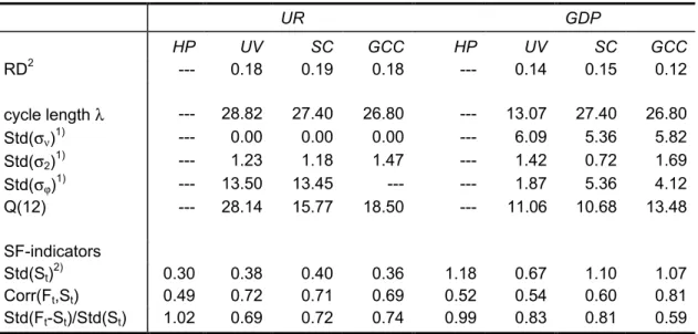
The results for the various STS models, all estimated with a smooth trend, are summarised in Table 1. As a benchmark, Table 1 also presents HP filter estimates with the usual smoothing parameter of τHP = 1600. Generally, apart from the univariate GDP model, the key parameters of the models correspond quite closely. The SF-indicators exhibit improved values for the SC and GCC models compared to the HP filter with the GCC model outperforming the SC one. The higher degree of correspondence between the smoothed and filtered estimates is also reflected in the graphs of the particular cyclical components, as shown in Fig. 1 to 3. In order to visualise the effect of the GCC restriction, Fig. 4 also shows the smoothed estimate of the UR cycle, reversed and standardised to the same variance as the GDP cycle.

7 More specifically, we comprise equations (4) in one single state-space form and introduce the covariances E(ηt(y,ϕ)ηt(ur,ϕ)) = E(ηt(y,ϕ)*ηt(ur,ϕ)*) as off-diagonal elements in cov(ηηt). All other off-diagonal elements of cov(ηηt) are restricted to zero.

(16)

Table 1: HP filter and STS models

UR GDP

HP UV SC GCC HP UV SC GCC

RD² --- 0.18 0.19 0.18 --- 0.14 0.15 0.12

cycle length λ --- 28.82 27.40 26.80 --- 13.07 27.40 26.80

Std(σ_ν)¹⁾ --- 0.00 0.00 0.00 --- 6.09 5.36 5.82

Std(σ2)¹⁾ --- 1.23 1.18 1.47 --- 1.42 0.72 1.69

Std(σ_ϕ)¹⁾ --- 13.50 13.45 --- --- 1.87 5.36 4.12

Q(12) --- 28.14 15.77 18.50 --- 11.06 10.68 13.48

SF-indicators

Std(St)²⁾ 0.30 0.38 0.40 0.36 1.18 0.67 1.10 1.07 Corr(Ft,St) 0.49 0.72 0.71 0.69 0.52 0.54 0.60 0.81 Std(Ft-St)/Std(St) 1.02 0.69 0.72 0.74 0.99 0.83 0.81 0.59 Note: RD² denotes the ratio of explained to total variance of the differenced series.

σν , σ2 , and σϕ denotestandard deviations of the irregular component and the innovations in the slope and the cycle.

Q(12) is the Ljung-Box statistics for autocorrelation in prediction errors (χ122 ) St and Ft denote smoothed and filtered estimates of the cycles.

1) values for UR multiplied by 100, for GDP by 1000.

2) values for GDP multiplied by 100.

While the near-rejection of the GCC restriction might stem from an under-parameterisation of the bivariate process for GDP and UR cycles, a more likely reason seems the sharp rise in the unemployment rate between 1981 and 1983. The models might tend to fix the UR trend somewhat too smooth in this period and attribute some part of the trend to the cyclical component in the unemployment rate. As a consequence, in the GCC model the size of the GDP cycle is then overestimated also.⁸ In turn, potential output growth rates exhibit somewhat higher volatility, compared to the SC model. The rise in the unemployment rate in this period might also be the reason for some significant autocorrelations in the prediction errors for the unemployment rate that appear in all models (see the statistics Q(12) in Table 1).

8 In order to address this point, we added a dummy variable to the UR trend allowing for two break points, i. e.,

∆²urttr = dt + ηt(ur,2), with the dummy dt set to 1 for some t, (e. g., 1981q2) and to -1 for some t+k (e. g., 1982q3).

For a reasonable range of different break points the dummy is highly significant and the GCC restriction is easily accepted (see Harvey and Koopman (1992) for the detection of outliers in STS models).

(17)

Table 2: Likelihood Ratio-Tests⁹

H1 H0 LR df p Correlation among cycl. shocks BV UV 19.85 1 <.001

SC restriction BV SC 0.03 1 .86

RW in GDP trend SC_RW SC 0.12 1 .72

GCC restriction GCC 3.52 1 .06

phase shift ω GCC CC 6.91 1 .01

3.2. Price and Wage Equations

The order of integration of prices and wages is a matter of debate in the relevant literature (e.g., Baillie and Chung, 1996). While augmented Dickey-Fuller (ADF) tests cannot reject the hypothesis that prices and wages are integrated of order two also for Austrian data, for the purpose of modelling Phillips curve type relationships there are nevertheless arguments for using equations in first differences.¹⁰ We will present results for equations in both first and second differences. The specification of the particular equations is based on SUR estimates using the filtered cycles, as obtained from ML-estimation, as explanatory variables. Since the system is recursive, this two-step estimation procedure provides consistent parameter estimates (and therefore good starting values for ML-estimation), though the standard errors are biased (Pagan, 1984). The wage equation in first differences is of standard kind. It is difficult to find a reasonably parsimonious price equation for Austria, however.¹¹ In equations in second differences, the only link between prices and wages is given in the wage equation by the labour share of income both in levels and first differences. This specification may be interpreted in terms of Johansen’s (1995) second-order co-integration. Table 3 presents final ML-estimates for two models, i.e., the GCC model extended by the wage equation in first differences (GCC_∆w) with the GDP cycle as explanatory variable, and the SC model extended by equations in second differences (SC_∆2wp).

9 The distribution of the LR-test of SC against SCRW is given by 1/2 χ12 (see Harvey, 1989).

10 Both specifications are used in the literature. As examples for equations in first differences see Adams and Coe (1990), Franz and Gordon (1994), and Coe (1985). For equations in second differences see Cote and Hostland (1994).

11 p, w, and q have been seasonally adjusted by forming fourth differences. While, in the wage equation, consumer prices (∆pc) appear to have higher explanatory power than the GDP deflator (∆p), the latter enters the equation through the labour share of income. The data also support a specification where ∆²pct-1 is used as a proxy for surprises in inflation (Layard, Nickell and Jackman, 1991). The failure in finding a parsimonious price equation has to do with the high dependency of Austrian on German prices. However, for several reasons we refrained from using German prices a explanatory variables.

(18)

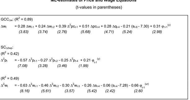
ML-estimates of Price and Wage Equations (t-values in parentheses)

GCC∆w: (R² = 0.89)

∆wt = 0.28 ∆wt-1 + 0.24 ∆wt-2 + 0.39 ∆²pct-1 + 0.51 ∆pct-4 + 0.28 ∆qt-4 - 0.21 (st-8 - 7.30) + 0.31 ϕ t-1(y) (3.83) (3.74) (2.76) (5.68) (4.71) (5.24) (2.98)

SC∆2wp: (R² = 0.42)

∆²pt = - 0.57 ∆²pt-1 - 0.27 ∆²pt-2 - 0.25 ∆²pt-4 + 0.21 ϕ_t-1^(y) (7.08) (3.28) (3.46) (1.99)

(R² = 0.49)

∆²wt = - 0.63 ∆²wt-1 - 0.46 ∆²wt-2 - 0.30 ∆²wt-3 - 0.26 ∆st-4 - 0.06 (st-4 -7.28) - 0.66 ϕ_t-1^(ur) (8.16) (5.61) (3.57) (5.42) (2.42) (2.60

Table 3: Bivariate STS Models with Price and Wage Equations GCC∆w SC∆2wp

UR GDP UR GDP

RD² 0.18 0.12 0.20 0.15

cycle length λ 27.86 25.56

std(σ_ν)¹⁾ 0.00 5.75 0.00 5.38

std(σ2)¹⁾ 1.14 1.75 1.15 0.71

std(σϕ)¹⁾ --- 4.19 13.54 5.42

Q(12) 28.17 14.64 22.17 11.64

Std(S_t)²⁾ 0.42 1.27 0.33 1.15

Corr(F_t,S_t) 0.90 0.92 0.81 0.70

Std(Ft-St)/Std(St) 0.43 0.40 0.57 0.52 Note: for notation see Table 1

1) values for UR multiplied by 100, for GDP by 1000

2) values for GDP multiplied by 100

The coefficients of the cycles in price and wage equations are significant at the 5% level in all cases. As concerns the SC_∆2wp model, it is worth noting that, indeed, while GDP and UR cycles are significant in the price and wage equation respectively, this does not hold the other way round. While the smoothed estimates are affected only slightly, both models exhibit a higher correspondence of smoothed and filtered cycles, compared to the respective model without the wage-price block (Fig. 6). In particular, contrarily to the bivariate models, the 1979 boom is now largely detected already from the filtered estimate of the GCC∆w model. The

(19)

equations seem reasonably stable. CUSUM statistics do not indicate instabilities in either model at the 10% significance level (Fig. 7). We also added a random walk component to the wage equation in the GCC_∆w model, thereby allowing the constant term to change over time, but did not find evidence for time-variation. Finally, we tested for inflation neutrality in the GCC_∆w model as outlined in section 2.2. The changes in the slopes of the GDP and UR trends, ∆²y_t-k^tr and ∆²ur_t-k^tr, were added to the wage equations at lags 1 to 4. The LR-statistics (χ42) yield insignificant values of 0.79 and 6.43 for GDP and UR trends, respectively. Thus the property of inflation neutrality of the particular trends is not rejected though the higher value for the unemployment rate indicates that there might exist possible longer-term trade-offs between unemployment and real wages.

4. Conclusions

Each approach to decompose a series into its long-run trend and cyclical components necessarily needs a set of identifying restrictions. For STS models these are basically given by assumptions on the nature of the stochastic processes underlying the particular components, together with orthogonality restrictions. The above results suggest that the implementation of economically motivated restrictions is feasible in multivariate STS models and that it might improve the estimate of the current cycle.¹² While the univariate STS model for GDP supported a local linear trend plus noise model, the utilisation of the cyclical co- movement of GDP and the unemployment rate revealed a pronounced cycle and a smooth trend. Moreover, we found reasonably stable relationships between price and wage inflation and the cycle. In sum, we imposed the basic cyclical relationships as used in the production approach, however with estimation and testing in a maximum likelihood framework.

More generally, the results appear promising with respect to the applicability of multivariate STS models for the investigation of cyclical relationships. While vector autoregressions may be regarded as an approximation to STS models (Harvey, 1989), the latter have the advantage of providing more direct ways for modelling cyclical relationships. Moreover, since first differencing removes a major part of business cycle frequencies from the data, STS models might in some cases also provide tests of higher power.¹³ The higher flexibility of STS models might be illustrated by one further example, related to our work. Blanchard and Quah (1989) used GDP and the unemployment rate in a bivariate VAR and identified the trend

12 In fact, the finding that the utilisation of cyclical co-movements improves estimates of the GDP cycle is a rather general one. It is well-known that the Beveridge-Nelson decomposition gives reasonable results only in the multivariate case. Also, Adams and Coe (1990) reported a considerable improvement of their cyclical estimates when the information contained in price and wage movements was exploited in a full systems estimation..

13 From the gain function of the first difference filter it is evident that it attaches a weight of less than 0.5 to frequencies of around 20-25 quarters. At the same the variance of short term frequencies is increased with a factor of up to four. As, e. g., Baxter (1994) has pointed out and demonstrated with an empirical example, first differencing might therefore distort relationships at business cycles frequencies to a considerable extent.

(20)

component by some variant of the BN-decomposition. The generalised common cycles restriction is clearly similar with respect to the underlying rationale of utilising cyclical co- movements. However, the Blanchard and Quah (1989) approach requires UR to be stationary, while the STS approach does not. The latter might therefore be also applied to those European countries with high unemployment rates.

Finally, for our data the bivariate STS models support a smooth GDP trend with slowly changing slope. Such a trend is integrated of order 2. While this seemingly contradicts the results of unit root tests, various work has provided evidence for the view that it might be, in fact, consistent with them. Harvey and Jäger (1993) have shown by a simulation study that augmented Dickey Fuller tests are very unlikely to detect a possible second unit root. On the other hand, Perron (1989) has found that a unit root in US GDP is rejected, if one single appropriate break point is introduced in the deterministic trend component. In sum, this suggests that indeed a smooth trend might be a reasonable specification and that, in turn, the specification of the GDP trend as a random walk might provide overly volatile estimates.

(21)

References

Adams, C. and Coe, D. (1990), ‘A systems approach to estimating the natural rate of unemployment and potential output for the United States’, IMF Staff Papers 37 (4), 232- 293.

Baillie, R. and Chung, C. (1996), ‘Analysing inflation by the fractionally integrated ARFIMA- GARCH model’, Journal of Applied Econometrics 11, 23-40.

Barrell, R, Morgan, D., Sefton, J. and in’t Veld, J. (1994): The cyclical adjustment of budget balances, NIESR report series 8, National Institute for Economic and Social Research, London.

Baxter, M. (1994), ‘Real exchange rates and real interest rate differentials’, Journal of Monetary Economics 33, 5-37.

Blanchard, O. and Quah, D. (1989), ‘The dynamic effects of aggregate demand and supply disturbances’, American Economic Review 79, 655-673.

Boone, L. and Hall. S. (1995), ‘Signal extraction and estimation of a trend: a monte carlo study’, paper presented at the EEA conference, Prague 1995.

Canova, F. (1993), ‘Detrending and business cycle facts’, CEPR Discussion Paper 782.

Coe, D. (1985), ‘Nominal wages, the NAIRU, and wage flexibility’, OECD Economic Studies 5, 87-126.

Cote, D. and Hostland, D. (1994), ‘Measuring potential output and the NAIRU as unobserved variables in a systems framework’, in Bank of Canada, Economic Behaviour and Policy Choice under Price Stability, 357-411.

European Commission (1995b), ‘The commissions services’ method for the cyclical adjustment model of government budget balances’, European Economy 60, 35-90.

European Commission (1995a), ‘The composition of unemployment from an economic perspective’, European Economy 59, 125-145.

Evans, G. and Reichlin, L. (1994), ‘Information, forecasts and measurement of the business cycle’, Journal of Monetary Economics, 33(2), 233-254.

(22)

Franz, W. and Gordon, J. (1994), ‘German and American wage and price dynamics:

differences and common themes’, European Economic Review 37, 719-754.

Giorno, C.; Richardson, P.; Roseveare, D.; van den Noord, P. (1995), ‘Potential output, output gaps and structural budget balances’, OECD Economic Studies 24, 167-210.

Harvey, A. (1985), ‘Trends and cycles in macroeconomic time series’, Journal of Business and Economic Statistics 3, 216-227.

Harvey, A. (1989), ‘Forecasting, Structural Time Series Models and the Kalman Filter’, Cambridge University Press, Cambridge

Harvey, A.; Henry, B.; Peters, S; Wren-Lewis, S. (1986), ‘Stochastic trends in dynamic regression models. an application to the employment-output equation’, Economic Journal 96, 975-985.

Harvey, A. and Jäger, A. (1993), ‘Detrending, stylized facts, and the business cycle’, Journal of Applied Econometrics 8(3), 231-247.

Harvey, A. and Koopman, S. (1992), ‘Diagnostic checking of unobserved components time series models’, Journal of Economic Dynamics and Control 17(1-2), 263-287.

Hodrick, R. and Prescott, E. (1980), ‘Post-war U.S. business cycles: an empirical investigation’, Carnegie-Mellon University, Discussion Paper no. 451.

Johansen, S. (1995), ‘A statistical analysis of cointegration for I(2) variables’, Econometric Theory 11(1), 25-59.

Karras, G. (1994), ‘Sources of business cycles in Europe: 1960-1988’, European Economic Review 38, 1763-1778.

King, R., Plosser, C, Stock, J. and Watson, M. (1991), ‘Stochastic trends and economic fluctuations’, American Economic Review 81, 819-839.

King, R. and Rebelo, S. (1993), ‘Low frequency filtering and real business cycles’, Journal of Economic Dynamics and Control 17, 207-231.

Layard, R., Nickel, S. and Jackman, R. (1991), ‘Unemployment - Macroeconomic Performance and the Labour Market’, Oxford University Press.

Pagan, A. (1984), ‘Econometric issues in the analysis of regressions with generated regressors’, International Economic Review 25(1), 221-246.

(23)

Perron, P. (1989), ‘The great crash, the oil price shock and the unit root hypothesis’, Econometrica 57(6), 1361-1401.

Pichelmann, K. (1993), ‘Die Bekämpfung der Arbeitslosigkeit in den OECD-Staaten aus österreichischer Sicht’, mimeo, Institute for Advanced Studies, Vienna.

Röger, K. (1994), ‘Output gaps based on a production function’, internal note, European Commission DG II.

Rosenberg, B. (1973), ‘Random coefficient models’, Annals of Economic and Social Measurement 2, 399-428.

Rünstler, G. (1996), ‘Common cycles in multivariate structural time series models’, IAS economic series, forthcoming, Institute for Advanced Studies, Vienna.

Sefton, J. (1995), ‘Output gaps and inflation: an approach using a multivariate Beveridge Nelson-decomposition’, NIESR discussion paper 87, National Institute for Economic and Social Research, London.

Torres, R. and Martin, J.P. (1990), ‘Potential Output in the seven major OECD countries’, OECD Economic Studies 14, 127-149.

(24)

Institut für Höhere Studien Institute for Advanced Studies Stumpergasse 56

A-1060 Vienna Austria

Phone: +43-1-599 91-145 Fax: +43-1-599 91-163