TiN films

TiN films

Dissertation

zur Erlangung des Doktorgrades der Naturwissenschaften (Dr. rer. nat.)

Fakult¨ at f¨ ur Physik Universit¨ at Regensburg

vorgelegt von Klaus Kronfeldner

aus Bogen

Durchgef¨ uhrt am

Institut f¨ ur Experimentelle und Angewandte Physik der Universit¨ at Regensburg

unter Anleitung von Prof. Dr. Christoph Strunk

November 2016

Das Promotionskolloquium fand statt am:

Pr¨ ufungsausschuss: Vorsitzender: Prof. Dr. Vladimir Braun

Erstgutachter: Prof. Dr. Christoph Strunk

Zweitgutachter: Prof. Dr. Ferdinand Evers

Weiterer Pr¨ ufer: Prof. Dr. Christian Back

1 Introduction 5 2 Fundamental ideas about the superconductor-insulator transition (SIT) 9

2.1 Superconductivity . . . . 9

2.1.1 Ginzburg-Landau equation . . . . 10

2.1.2 Bardeen-Cooper-Schrieffer theory . . . . 12

2.1.3 Josephson effect . . . . 13

2.2 Superconductivity in thin films . . . . 14

2.2.1 Berezinskii-Kosterlitz-Thouless transition . . . . 14

2.2.2 Superconducting fluctuations . . . . 15

2.2.3 Vortex-based resistive mechanisms . . . . 21

2.2.4 Phase slip centers and heating in superconducting thin films . . 23

2.3 Superconductor-insulator transition . . . . 30

2.3.1 Two-dimensional superconducting systems under the influence of disorder . . . . 30

2.3.2 Phenomenology of the disorder- and field-driven SIT . . . . 34

2.3.3 The SIT as a quantum phase transition (QPT) . . . . 38

2.3.4 Josephson-junction-array model . . . . 42

3 Materials and Methods 49 3.1 Sample Properties . . . . 49

3.2 Measurement Setup . . . . 54

4 Multiple crossovers of magnetoresistance isotherms 59 4.1 Phenomenological description of the three crossing points . . . . 62

4.1.1 Low temperatures (LT) . . . . 62

4.1.2 Medium temperatures (MT) . . . . 64

4.1.3 High temperatures (HT) . . . . 66

4.2 Scaling behaviour near the crossing points . . . . 67

4.2.1 The finite size scaling approach . . . . 67

4.2.2 Alternative scaling approach for the MT regime . . . . 68

4.2.3 Alternative scaling approach for the LT regime . . . . 69

4.2.4 Coexistence of superconducting and insulating behaviour in IV curves near to B

. . . . 71

5 Superconducting fluctuations above B

73

6 Test for long-ranged interactions with a screening top-gate 79 6.1 General characterization of the sample properties at low temperatures . 82 6.2 Experimental test for a screening effect due to a metallic top-gate . . . 83 7 Disorder driven Superconductor-Insulator transition in TiN 87

7.1 Heating phenomena at zero magnetic field for differently disordered sam- ples . . . . 87 7.2 Hysteretic jumps in insulating IV characteristics . . . . 98 7.3 R(T ) and critical temperature at zero magnetic field on approach of the

D-SIT . . . 103 8 Size-dependent superconductor-insulator transition 111 8.1 Size dependence of the superconducting transition at zero magnetic field 112 8.2 Size dependence of the magnetic-field-driven SIT . . . 118

9 Discussion 125

9.1 Multiple criticality vs. multiple crossovers - finding the point of the QPT125 9.2 Disorder driven SIT and the vortex BKT physics . . . 132 9.3 Duality of superconducting and insulating states . . . 134

10 Summary and Outlook 137

Bibliography 141

It is well known that the resistance of many bulk-metals sharply drops to zero below the critical temperature T

. In the case of disordered thin films, T

is lowered compared to the bulk critical temperature and additionally the decrease of the resistance below T

is broadened to a certain temperature range. The temperature at which the resistance vanishes completely is known as the Berezinskii-Kosterlitz-Thouless (BKT) transition.

This years Nobel price goes to Kosterlitz and Thouless particularly for the finding of the vortex-antivortex binding-unbinding transition [1, 2] based on the preceding publications of Berezinskii [3, 4]. This award demonstrates the importance of the physics in two dimensional superconductors for today’s science.

However, disordered metallic thin films that can form a superconducting phase at low temperatures are by no means fully described by the physics of the BKT transition.

At high temperatures the conductivity σ can be described by the Drude expression

σ = ne

τ /m, (1.1)

where m is the mass of the electrons, n is the charge carrier density, −e is the electron charge and τ is the scattering time. Upon lowering temperature localization effects occur. The electrons get more and more localized due to coherent backscattering and disorder-enhanced electron-electron interactions [5]. Above T & T

, superconducting fluctuations lower the resistance R. Within the mean-field theory of superconduct- ing fluctuations the resistance would drop to zero at T

. But in the BKT phase, where unbound vortex-antivortex pairs can freely move across the superconducting thin film, the resistance stays finite. Finally at T

, the BKT transition temper- ature, the resistance vanishes completely and the vortex-antivortex pairs are bound together. Between the temperature regions where either electron localization or su- perconducting fluctuations or BKT physics dominate the temperature dependence of the resistance, continous descripitions of the R(T ) dependence under the influence of multiple effects are necessary. It is a tough challenge to identify the regions in the temperature dependence of the resistance that are dominated by different effects.

In some materials, such as titanium nitride (TiN) or indium oxide, a highly insulating state occurs upon increasing disorder or magnetic field B . Instead of a decrease of the resistance at low temperatures, an increase is observed. This transition is called superconductor-insulator transition (SIT). This increase of the resistance is supposed to be caused by a localization of Cooper pairs instead of a localization of electrons.

Measurements of the local density of states near the disorder driven SIT (D-SIT) lead

to this conclusion [6].

The SIT is considered to be a second order quantum phase transition which is also called a continuous quantum phase transition. Continuous quantum phase transitions are driven by the change of a single parameter in the Hamiltonian of the system. The superconducting ground state is formed by a condensate of Cooper pairs and excita- tions in form of vortices. The insulating state is can be visualised by a condensate of vortices and the excitations are hopping Cooper pairs [7]. Either disorder or magnetic field is the parameter that induces the phase transition. The change from a Cooper pair condensate to a vortex condensate is suggested by a duality transformation where con- ductivity is replaced by resistivity. Based on general properties of continous quantum phase transitions at finite temperatures, the theory of finite size scaling was adapted to the SIT [7, 8]. A signature of a superconductor-insulator quantum phase transition are critical values for disorder and magnetic field, at which the resistance is temperature independent. Such a plateau in the R(T ) dependence is accompanied by a crossing point in the magnetoresistance isotherms. Crossing points in the R(B) isotherms are extensively discussed in the context of a quantum phase transition. Though, the found apparent intersection points are not an unambiguous evidence for a quantum phase transition. Superconducting fluctuations can cause approximate crossing points in the magnetoresistance isotherms [9]. Multiple crossing points are already found in Refs.

[10, 11]. There a finite size scaling analysis was pursued and to each crossing point in the R(B) isotherms a different type of the quantum phase transition was attributed.

Artificial Josephson junction arrays consist of superconducting islands coupled by Josephson weak links. Two competing energy scales deterimine the conductivity of the array. On the one side the Josephson energy E

favours charge transport, on the other side the charging energy E

forms an energy barrier the Cooper pairs have to overcome to move. The increase of the ratio E

/E

induces a SIT. As both energy scales are tunable by the geometry and E

can be tuned by an applied magnetic field, Josephson junction arrays offer a more controllable access to the SIT than disordered thin films. From the measured fluctuation of the local superconducting energy gap across a TiN film [6], the formation of superconducting islands that are embedded in a normalconducting matrix is likely to lead to the SIT in TiN. The similarity of such a natural array to artificial Josephson junction arrays, motivated the explanation of the SIT in TiN in terms of a competing E

and E

.

Dual to the vortex BKT on the superconducting side of the SIT, the charge BKT was postulated in the insulating state of Josephson junction arrays. An Arrhenius law which describes a temperature activated R(T ) dependence was found to be to weak for the R(T ) curves presented in Refs. [12, 13]. The convex shape of the R(T ) dependence in the Arrhenius plot was attributed to the charge BKT. In TiN thin films a similar behaviour was found which was called “hyperactivated” [14] and the new highly insulating phase was called “superinsulator” [15].

In this thesis differently disordered samples of different lateral sizes were measured at

low temperatures and magnetic fields ranging from zero up to B = 17 T. A thorough

investigation of the disorder-driven as well as the magnetic field induced SIT was

pursued on the basis more than 700000 measurement files where most of these files

contain recorded current-voltage characteristics.

main results of this work are splitted into five chapters. Chapter 4 contains the three found crossing points in the magnetoresistance isotherms and phenomenological de- scriptions of the R(T, B) dependences in the three corresponding temperature regimes.

A finite size scaling analyis is included. In chapter 5 superconducting fluctuations ac- cording to the theory of Galitski and Larkin [16] are found to well describe the magne- toresistance isotherms at high magnetic fields. Tests for a electrostatic screening effect due to a metallic top-gate are discussed in chapter 6. In chapter 7 heating phenomena in the IV characteristics, the evolution of the critical temperature T

and the evolution of the BKT transition temperature T

are investigated in the vicinity of the D-SIT.

The application of a special measurement technique enabled to find a dual shape of the IV characteristics in the insulating state with interchanged current and voltage axes with respect to the superconducting IV characteristics. In chapter 8 the size de- pendence and the disorder dependence of both T

in the superconducting state and the activation energy in the field-driven insulating state are revealed. In the discussion in chapter 9 the results of chapters 4, 5, 6, 7, 8 are dicussed in a comprehensive way.

The results are discussed in the light of to recent publications. Chapter 10 summarizes

the obtained results and gives an outlook.

superconductor-insulator transition (SIT)

2.1 Superconductivity

In 1911 Heike Kamerlingh Onnes discovered superconductivity while he studied the resistivity of pure metals at low temperatures [17]. When he and his coworker van Holst measured the resistivity of a mercury sample, they noticed a sharp drop in resistance below 4.2 K. They found that below a characteristic critical temperature T

many materials became perfectly conducting. These superconducting samples were not only perfect conductors, they were perfect diamagnets as well, which was found by Meissner and Ochsenfeld in 1933 [18]. In the observed Meissner phase a magnetic field is expelled completely from the inside of a superconducting bulk of a Type I superconductor.

Within a penetration depth λ the magnetic field is screened exponentially from the interior of the superconductor. The penetration depth λ

can be derived from the London equations for electrical field E, magnetic field B and the density J

of the supercurrent

E = µ

λ

∂

∂t (j

) (2.1)

B = −µ

λ

curl(j

) (2.2)

where n

is the number density of superconducting electrons. The Maxwell equation curl H = j, where B = µµ

H with µ ≈ 1, combined with the second London equation 2.2 leads to

∇

B = B

λ

(2.3)

where the London penetration depth λ

is given by λ

=

r m

(2e)

µ

n

. (2.4)

The Meissner phase vanishes at a critical field B

above which the sample is nor-

mal conducting. The critical field is thermodynamically connected to the free energy difference between the normal and superconducting states:

f

(B = 0, T ) − f

(B = 0, T ) = B

2µ

(2.5)

The following introduction to the basics of superconductivity is taken from [19, 20].

2.1.1 Ginzburg-Landau equation

Based on Landau’s theory of second order phase transitions, Ginzburg and Landau expanded the free energy with respect to a complex order parameter ψ = |ψ|e

with the local density of superconducting electrons

n

= |ψ(x)|

(2.6) The free energy is then given by

f = f

+ α|ψ|

+ β

2 |ψ|

+ 1

2m |(−i ~ ∇ + 2eA) ψ|

+ 1

2µ

B

(2.7) with α(t) = α

(t − 1) around T

where t = T /T

and with the positive constants α

and β. If α is positive, the minimum free energy occurs at |ψ|

, which corresponds to the normal state. For α < 0 the minimum occurs at

|ψ|

= |ψ

| ≡ − α

β (2.8)

where ψ

is used because ψ reaches this value infinitely deep in the interior of the superconductor, where all surface currents and fields are screened. The Ginzburg- Landau differential equations are found by minimizing the free energy with respect to ψ and A:

αψ + β|ψ|

ψ + 1

2m (−i ~ ∇ + 2eA)

ψ = 0 (2.9) j

= ie ~

m (ψ

∇ψ − ψ∇ψ

) − 4e

m |ψ|

A (2.10)

Inserting |ψ|

= −α/β in Eq. 2.10, the second London equation 2.2 is obtained and the Ginzburg-Landau expression for the penetration depth λ is

λ

= s

mβ

4µ

e

|α| (2.11)

The Ginzburg-Landau coherence length ξ

is introduced as a the characteristic dis-

tance over which spatial changes in ψ occur:

ξ

= ~

p 2m|α| (2.12)

From the first Ginzburg-Landau equation 2.9, without a magnetic field, the spatial variation of ψ and accordingly n

on the boundary of a superconductor is:

ψ(x) ψ

= tanh x

√ 2ξ

(2.13)

Fig. 2.1: At the boundary between a normal metal and a superconductor the magnetic field B and the superconducting wave function spatially varies according to the Ginzburg-Landau theory (from [20]).

It is useful to introduce the dimensionless Ginzburg-Landau parameter κ = λ/ξ

. For κ < 1/ √

2 the material is a type I superconductor, for κ > 1/ √

2 it is a type II superconductor. In a type I superconductor no vortices can exist in the interior, the superconducting state is a Meissner state and the sample becomes normal conducting above B

(Eq. 2.5). In a type II there are two critical fields. Above B

supercon- ducting vortices penetrate the Meissner phase with a flux quantum φ

= h/2e. The so called Shubnikov phase holds up to a critical field B

which is determined by the maximum density of vortices. At B

the area per flux quantum is 2πξ

, therefore the critical field above which superconductivity vanishes is

B

= φ

2πξ

(2.14)

2.1.2 Bardeen-Cooper-Schrieffer theory

The superconducting state could be explained microscopically for the first time by Bardeen Cooper and Schrieffer [21] in 1957. Here just the basic concepts and the main results are given. A weak attractive interaction between electrons mediated by electron-phonon interaction leads to the formation of bound pairs of electrons. Within these pairs the electrons occupy states with equal but opposite momentum and spin.

These bosonic pairs are called Cooper pairs and they condense to a superconducting ground state in which the pair energy is lowered by the energy gap ∆ compared to the Fermi energy of the normal Fermi sea without electron-phonon interaction. The su- perconducting ground state quantum-mechanically forms a macroscopic wave function.

From this quantum-mechanical interpretation of superconductivity many features of superconducting materials could be explained and also predicted. The Cooper pair size ξ

could be estimated to be

ξ

= ~ v

π|∆| (2.15)

with v

the Fermi velocity. The minimum energy required to break a pair, creating two quasiparticle excitations is for T T

E

(T = 0) = 2∆(T = 0) = 3.528k

T

(2.16) with E

= 2∆ the energy gap which tends to zero for T → T

:

∆(T )

∆(0) ≈ 1.74

1 − T T

T ≈ T

(2.17)

From the BCS theory the behaviour of the penetration depth λ can be deduced for a number of important cases, such as thin films. In parallel magnetic field the super- current response of a nonlocal (BCS) thin-film (d λ) superconductor is equivalent to that of a local (London) superconductor with an effective penetration depth

λ

= λ

(ξ

/d)

(for d ξ

) (2.18) with film thickness d, the London penetration depth (Eq. 2.4) and ξ

is the modified Pippard coherene length. When a magnetic field is applied perpendicular to a thin film the penetration depth is modified to

λ

= λ

/d (2.19)

which is also known as the Pearl penetration depth. Werthamer, Helfand, and Ho-

henberg [22] evaluated the temperature dependence of the upper critical field H

of

type II superconductors based on a BCS model where Pauli spin paramagnetism and

spin-orbit impuritiy scattering is included.

ln 1 t =

1

2 + iλ

4γ

· ψ 1

2 +

¯ h +

λ

+ iγ

2t

+ 1

2 − iλ

4γ

· ψ 1

2 +

¯ h +

λ

− iγ

2t

− ψ 1

2

(2.20)

where ψ is the digamma function, γ

≡ [(α ¯ h)

− (

λ

)

]

, t = T /T

, ¯ h = 2eH(v

τ /6πT

), α = 3/2mv

τ and λ

= 1/3πT

τ

. With τ

= τ

+τ

and (τ

, τ

) are the scattering times for spin-independent and spin-orbit scattering respectively. H is the magnetic field and v

is the Fermi velocity. α includes the effect of Pauli spin paramagnetism and λ

includes spin orbit effects. T

is the highest temperature for which the Usadel-equations [23] have non-trivial solutions. The diffusion-like Usadel- equations are only valid for a superconductor of type II in the dirty limit.

With Eq. 2.20 it is possible to calculate t = T /T

at a known magnetic field H.

Since this field H is the critical field H

at the given t, H

(T ) can be obtained. For our TiN thin films H

(T ) can be approximated within 1% by (Tatyana Baturina, personal communication):

H

(T ) = H

(0) · cos π 2 ·

T T

!

(2.21)

2.1.3 Josephson effect

A weak link connecting two superconducting electrodes is called a Josephson junction.

The weak link can be a thin insulating layer, a thin normal metal layer or a short narrow constriction of in otherwise continuous superconducting material. In such geometries the ac- and dc-Josephson effects occur. In a Josephson junction a supercurrent I

flows which is driven by the phase difference ∆φ of the Ginzburg-Landau wave function in the two superconducting electrodes:

I

= I

sin ∆φ (2.22)

with I

the Josephson critical current, the maximum supercurrent through the junction.

Eq. 2.22 is the first Josephson equation. For an externally applied voltage V across the junction the ac-Josephson effect with an alternating current of amplitude I

and frequency ν = 2eV /h across the junction appears. The ac-Josephson effect is desribed by the second Josephson equation

d(∆φ)/dt = 2eV / ~ . (2.23)

2.2 Superconductivity in thin films

2.2.1 Berezinskii-Kosterlitz-Thouless transition

In two dimensional superconducting films (d ξ) even at zero magnetic field vor- tices spontaneously can be generated below the mean-field critical temperature T

. The energy cost of the creation of a single pancake vortex (field axis perpendicu- lar to the film-plane) of volume ∼ πξ

d is E

= (H

/2µ

)4πξ

d ln κ. With ξ(T ) = φ

/2 √

2H

(T )λ

(T ) from the Ginzburg-Landau theory and with Eq. 2.19 we obtain:

E

=

φ

4πλ

µ

ln

λ

ξ

(2.24) If the sample size with radius R in a simplified model is smaller than λ

, the logarithm in Eq. 2.24 is substituted by ln(R/ξ). In the Berezinskii-Kosterlitz-Thouless (BKT) phase vortex-antivortex pairs with opposite circulation sense are generated by thermal activation. For an intervortex separation of ∼ R

, the creation energy of such a pair of vortices is not double the value of E

, instead of the sample size R the length R

sets the total energy of the vortex-pair:

E

= 2 ·

φ

4πλ

µ

ln

R

ξ

(2.25) The energy hence increases with increasing distance of the vortices with ∼ ln(R

/ξ) which results in an attractive force between the vortex-antivortex pair. For R

∼ ξ the vortex cores are touching and the vortices annihilate each other. In thermal equilib- rium for temperatures T

< T < T

the annihilation and creation processes occur with the same frequency. Below T = T

, the vortex BKT transition temperature, no thermally activated unbinding of vortex-antivortex pairs appears. T

is deter- mined by the balance of entropy gain that results from the two rather independently moving vortices for T > T

compared to pair-like bound vortices for T < T

and the energy cost for creation of the vortex pair:

k

T

≈ φ

8πλ

µ

(2.26)

A current flow through the sample in the BKT phase leads to flux-flow resistance due to the movement of the unbound vortex-antivortex pairs, followed by a motion of the vortices in opposite directions until they disappear at opposite edges of the sample.

According to Halperin and Nelson the temperature dependence of the resistance in the BKT regime reads [24, 25]

R(T ) ∝ exp − b

(T /T

− 1)

!

(2.27)

where b is a constant of the order of unity. In the vortex BKT regime the resistance is linear as there is an equilibrium population of unbound vortices. Below T

there are no free vortices for zero driving current. The number of vortices that are created by a finite current I increases as I

just below T

. Therefore there is no linear resistance below T

, the voltage V rises with a powerlaw V ∼ I

with α(T

) ≈ 3 at T

. Beasley, Mooij and Orlando found a relationship between the BKT transition temperature and the sheet resistance in the normal state R

[26]:

T

T

·

f

T

T

= 0.561 π

8

~ e

1

R

(2.28)

where f T

T

= ∆(T )

∆(0) tanh

β∆(T )T

2∆(0)T

(2.29) However it is not always clear how to determine the resistance R

. A plot of R

vs.

T

/T

that is calculated with Eqs. 2.28 2.29 is shown in Fig. 9.3b. In [27] the sheet resistance at room temperature and the maximum resistance in the temperature dependence of the resistance at zero magnetic field are discussed to be taken for R

. In Ref. [28] the extrapolated zero-temperature value of the normal state resistance R

is argued to be a useful approximation for R

in Eq. 2.28. The extrapolated value of R

was obtained under usage of the phenomenological description of σ ∝ T

for T T

[29].

2.2.2 Superconducting fluctuations

In the BCS model right at the mean field critical temperature T

a finite amplitude of the order parameter forms. In contrast, the resistivity of thin films does not vanish until it is cooled below the vortex BKT transition temperature T

which can be estimated according to Eq. 2.26 (see chapter 2.2.1). For temperatures exceeding T

(B ) with B > B

(T ), superconducting fluctuations contribute to the conductivity of 2D films.

Additionally, above T

, electron localization effects have to be considered, such as weak localization and disorder enhanced interelectron interference due to the Aronov- Altshuler effect [5]. The weak localization effect concerns the diffusive motion of single electrons. An electron that is at time t = 0 at the place r = 0 takes part in the diffusion motion with Fermi velocity v

and mean free path l = v

τ , where 1/τ is the frequency of the elastic scattering events. The probability for the electron to be found at a position r after a time t τ is given by the classical expression

p(r, t) = (4πDt)

e

, r

=

d

X

1

x

, Z

p(r, t)dr = 1 (2.30)

where d is the dimension of the system and D = lv

/d is the diffusion coefficient. The

classical return probability for an electron in a 2D system to come back to the place

r = 0, within the characteristic time τ

for loosing the phase memory due to inelastic

scattering, is p(0, τ

) = (4πDτ

)

. For t < τ

an electron that passes the same place twice, interferes with itself. Since this interference is of a quantum mechanical nature, the probability for finding the electron at this place is double of that for a classical diffusive description. As a result of the interference, the conductivity is lowered. With growing disorder the mean free path l = v

τ

shrinks due to a smaller mean time τ between the elastic scattering events. In consequence the diffusion coefficient decreases and with that the classical return probability p(0, τ

) increases. The enhanced p(0, τ

) due to increasing disorder leads to a higher correction to conductivity originated from weak localization.

The Aronov-Altshuler effect in contrast, results from the interelectron interference of two different electrons that meet twice. The requirement for the constructive inter- ference of two electrons is the same phase of the wave functions for both electrons at a time t = 0. The characteristic time τ

within phase coherence of the two electrons which have the same phases at t = 0 is conserved, depends on the energy difference

∆ of the two electrons. Only electrons with energies around the fermi level E

take part in the diffusion motion with

E

− k

T . . E

+ k

T. (2.31) Under this condition the characteristic dephasing time is τ

' ~ /k

T . As a conse- quence the interelectron interference effect becomes stronger at lower temperatures.

The size of the interference region can be estimated to L

' l τ

τ

' v

~ τ

T

' r

~ D

T . (2.32)

The collision frequency of two electrons with diffusive motion is described as

~

τ

∼ 1

g

L

(2.33)

where g

∼ E

m

is the density of states at the fermi level, d is the dimension of the system and m is the electron mass. Since for a disordered system τ

τ, the collision of electrons does not directly make a noticeable contribution to conductivity.

However, the interelectron interaction in the diffusion channel reduces the density of states for around the fermi level to

∆g(T = 0, ) ∼ ( ~ D)

· ln τ

~

(2.34) for a two-dimensional system at zero temperature T . With increasing disorder, τ and D decrease and in consequence the reduction of the density of states ∆g is stronger.

For both weak localization and interelectron interference effects, the temperature

dependence of the correction to conductivity is logarithmic with

∆G

= ∆G

+ ∆G

= G

(αp + B) ln

k

T τ

~

= G

A ln

k

T τ

~

(2.35) where A = αp + B and G

= e

/(2π

~ ) ' (81 kΩ)

. The term with αp originates from the weak localization effect and the term with B from the interelectron interaction (see Eq. 2.41). B is of order unity. The parameter p is given by 1/τ

∝ T

and the parameter α is given by α = 1, −1/2, 0 for the potential, spin-orbit and spin scattering, respectively.

term expression

WL + AA ∆G

= G

A ln

k

T τ

~

AL ∆G

= e

16 ~ T T − T

DOS ∆G

= G

ln

ln(T

/T ) ln(k

T

τ / ~

MT ∆G

= G

β(T ) ln T τ

~

DCR ∆G

= 4

3 G

ln ln 1

T

τ − ln ln 1 T

Table 2.1: Corrections to conductivity for the diffusion channel (WL + AA) and for the Cooper channel. For the Cooper channel the Aslamazov-Larkin term (AL), the correc- tion to the conductivity due to the depression of the density of states (DOS), the Maki- Thompson contribution (MT) and the correction to the conductivity originated from the renormalization of the single particle diffusion coefficient (DCR) are listed. The calculated temperature dependences for the seperate corrections to conductivity as well as the total conductivity, where all the corrections are summed, are shown in Fig. 2.2a. The prefactor G

= e

/(2π

~) ' (81 kΩ)

is usually taken to be the maximum correction to conductivity due to fluctuations. It is connected to k

l = 1 which is a lower limit (and hence an upper limit for disorder) for the applicability of perturbative corrections to conductivity.

A differentiation of weak localization and the Aronov Altshuler effect is only possible under an applied magnetic field, where the correction to conductivity due to weak localization vanishes but the Aronov Altshuler contributions are not affected.

Superconducting fluctuations arise due to the interaction of electrons with nearly

opposite momenta, called Cooper channel. Terms of the following four types describe

the fluctuation conductivity [27]: 1) Aslamazov-Larkin (AL) term which is connected

with the direct conductivity of the fluctuating Cooper pairs. The AL contribution to conductivity is positive; 2) Due to the AL-type of fluctuations above T

, the number of normal electrons decreases. The density of states term (DOS) describes the decrease of the conductivity of the electrons according to the Drude expression Eq. 1.1; 3) The presence of fluctuations, the renormalization of the single-particle diffusion co- efficient leads to another correction to conductivity (DCR); 4) The Maki-Thompson term (MT) is connected with coherent scattering of electrons on impurities. The re- sulting contribution to conductivity can either be positive or negative, depending on the conventional pair breaking parameter δ = π ~ /(8k

T τ

).

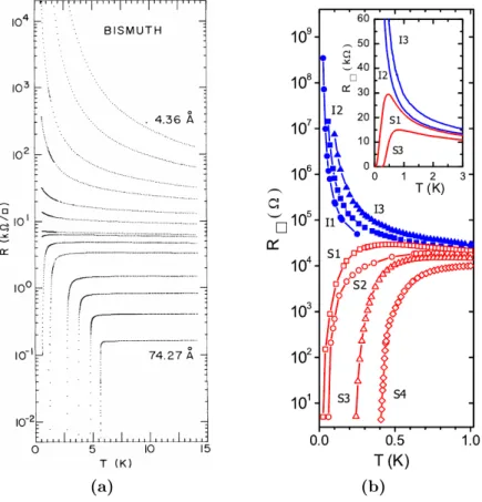
(a) (b)

Fig. 2.2: (a) Calculated temperature dependence of superconducting fluctuation contribu- tions to conductivity (in units of G

= e

/(2π

~ )) (image from [27] with theoretical expres- sions taken from [30]). The derived curves for AL, DOS, and DCR are universal functions of reduced temperature t = T /T

, the MT correction is presented for the convential pair break- ing parameters δ = 0.01 and δ = 0.05. The black solid lines are the sum of all contributions to superconducting fluctuations on a logarithmic temperature scale. The inset shows the same total sum on a logarithmic conductivity scale. (b) Measured resistance per square vs.

temperature for four differently disordered TiN film samples. Solid black lines correspond to

fits accounting for all the quantum contributions. The red dashed lines, marked as WL+ID,

are the separate contributions of the sum of weak localization and interparticle interaction to

the resistances of the samples S01 and S15. The blue dotted lines show the sum of corrections

due to superconducting fluctuations [27]).

In table 2.1 the contributions to conductivity from the diffusion channel as well as from the Cooper channel are listed. The Larkin factor β(T ) has the form [31]

β(T ) = π

4

X

m

(−1)

Γ

(|m|) − X

m≥0

Γ

(2m + 1) (2.36)

where m is an integer m = 0, ±1, ±2, ..., and Γ

(|m|) =

ln T

T

+ ψ 1

2 + |m|

2

− ψ 1

2

− ψ

1

2 + |m|

2

1 4πk

T τ

(2.37) with the digamma function ψ. For low temperatures ln(T /T

) 1 the expression for β(T, τ

) reduces to

β(T, τ

) = π

4

1

ln(T /T

) − δ (2.38)

where δ = π/(8k

T τ

is the Maki-Thompson pair breaking parameter.

In Fig. 2.2a the different contributions to conductivity for the four latter fluctuation types are calculated for given parameters. In Ref. [27] all the quantum contributions to conductivity mentioned in table 2.1 were taken into account for an anaysis of super- conducting fluctuations at zero magnetic field for a number of differently disordered TiN films. The theoretical expressions taken from Ref. [30] served as a comprehen- sive formula. The fit to measured R(T ) data is shown in Fig. 2.2b for the differently disordered TiN films.

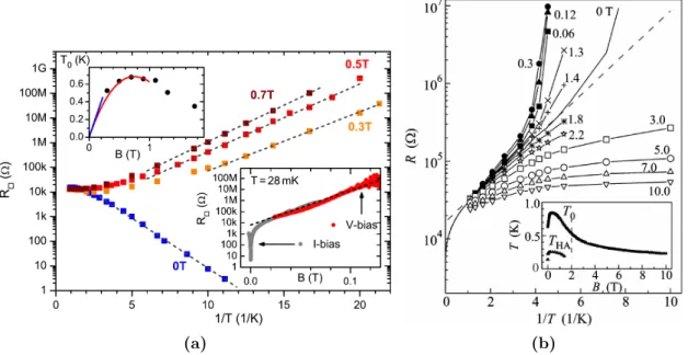
(a) (b)

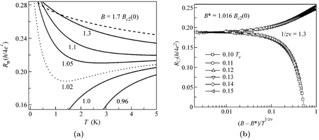
Fig. 2.3: (a) Fluctuating conductivity according to Eq. 2.39 as a function of magnetic field is plotted for four different temperatures (from [16]). Resistance per square (open symbols) vs. perpendicular magnetic field for a TiN sample deeply in the superconducting regime at various temperatures. Solid lines are plotted functions calculated on basis of Eq. 2.40 with B

(0) = 2.8 T and T

= 2 K (from [32]).

We now turn to the superconducting fluctuations at low temperatures T < T

above

the critical magnetic field B

. Galitski and Larkin evaluated the total correction to conductivity δσ for superconducting fluctuations above B

for T T

[16]. T

is the temperature at which an equilibrium concentration of Cooper pairs appears (the BCS transition temperature). Aslamazov-Larkin, Maki-Thompson and density of states contributions for the dirty case with T

τ 1 (where τ ist the scattering time) are concerned in the first (one-loop) approximation:

∆G

= 2e

3π

~

− ln r h − 3

2r + ψ(r) + 4[rψ

(r) − 1]

(2.39) where r = (1/2γ)h/t, γ = 1.781 is Euler’s constant, h = (B − B

(T ))/B

(0) and t = T /T

. B

(T ) = B

(0) · cos(π(T /T

)

/2) is an approximation of the Werthamer- Helfand B

(T ) [22] for TiN (Eq. 2.20). ψ is the digamma function with ψ(x) =

d

dx

ln(Γ(x)) =

, where Γ is the gamma function. ψ

is the trigamma function with ψ

(z) =

ln(Γ(z)). The total conductivity is calculated with

G(T, B) = G

+ ∆G

+ ∆G

. (2.40) with G

the normal state conductivity. ∆G

the correction to conductivity due to Aronov Altshuler type of interelectron interference [5]:

∆G

= G

B ln

k

T τ

~

(2.41) where B is a constant which depends on the Coulomb screening and it remains of the order of unity. In Fig. 2.3a the calculated magnetic field dependence of δσ for several values of t is depicted.

In Ref. [32] the magnetoresistance isotherms of TiN samples deeply in the supercon- ducting regime could be well described by the theory of superconducting fluctuations according to Eq. 2.40 (see Fig. 2.3b).

In subsequent works the result for the correction to conductivity of Eq. 2.39 was reproduced by Tikhonov, Schwiete and Finkelstein [33], based on the Usadel equation in the real-time formulation, and by Glatz, Varlamov and Vinokur [30], based on the perturbative first order fluctuation theory. Burmistrov, Gornyi and Mirlin [34]

evaluated a magnetoresistance behaviour that resembles Eq. 2.39. Their analysis is based on the renormalization group for a nonlinear sigma model. This approach is not restricted to the case of perturbative superconducting fluctuations that are small compared to the Drude conductivity. Though the latter three works reproduce the magnetoresistance above B

for low temperatures according to Eq. 2.39, the contributions to conductivity due to fluctuations in Ref. [34] differs from that in Refs.

[33, 30]. Tarasinski and Schwiete [35] generalized the results of Ref. [33] under usage

of a quasiclassical kinetic equation approach. They obtained an expression for the

correction to conductivity above B

similar to Eq. 2.39. Summarizing, Eq. 2.39 was

reproduced already several times [33, 30, 34, 35] with just slight modifications.

2.2.3 Vortex-based resistive mechanisms

Under an applied magnetic field which is perpendicular to the plane of the film, a superconducting disordered thin film with κ < 1/ √

2 is penetrated by vortices with a distance a

= (φ

/B)

. For an applied current through the superconducting film, the vortices move according to the Lorentz force, perpendicular to the current to the edges of the film. This movement induces an electric field which is parallel to the applied current and therefore acts like a resistive voltage. Pinning of the vortices to certain sites on the superconducting film can slow down the motion of the vortices. For strong pinning any substantial vortex motion is prevented and a supercurrent can flow up to a certain critical current, above which the Lorentz force overcomes the pinning forces.

For less strong pinning a variety of resistive mechanims due to vortex motion can be observed.

In a very simplified model Bardeen and Stephen estimated the flux-flow resistance, phenomenologically assuming a viscous drag coefficient η. The viscous force on a vortex with velocity v

is then ηv

. They found that η is related to the upper critical field H

and the normal state resistivity ρ

in the following way:

η ≈ φ

H

ρ

c

(2.42)

where c is the velocity of light in vaccum. For the flux-flow resistance ρ

they found ρ

ρ

≈ B H

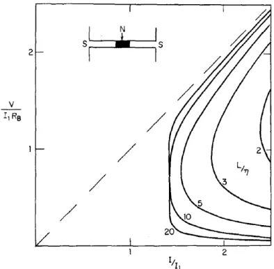
(2.43) Experimental data follows this linear dependence quite well, at least for small magnetic fields and low temperatures. Kim, Hempstead and Strnad [36] refined the theory of flux-flow resistance to explain the deviations from the linear dependence of Eq. 2.43 (see Fig. 2.4)

Fig. 2.4: ρ

/ρ

of a Nb-Ta specimen is shown as a function of magnetic field H at given

values of t = T /T

. H

(T ) is indicated by vertical arrows. The dashed line corresponds to

the Bardeen-Stephen flux-flow resistance (Eq. 2.43). For low temperatures and low magnetic

fields the linear dependence of Eq. 2.43 resembles the measured data. (from [36]).

Inui, Littlewood and Coppersmith [37] used a model of single vortex depinning to explain the experimentally observed temperature activated motion of vortices from homogeneous and densely distributed pinning centers. They treat the vortices inde- pendent of each other, with interaction included in the single-vortex dynamics. They justify this approach with the unusual softness of the flux lattice for localized deforma- tions, which occurs for large screening lengths and anisotropy. Inui et al. explicitly do not consider the possibility of collective pinning. For low temperatures they derived the barrier height for the temperature activated motion of vortices for two different types of field dependence:

V

≈

V

+ σ ln(H

/H), H H

, (2.44)

V

− π

γ/K

, H H

(2.45)

With a crossover field H

. H

and σ are some constants. γ ≈ dφ

H/128π

λ

where d is the coherence length perpendicular to the film. The logarithmic dependence in Eq.

2.44 results in a powerlaw of the magnetoresistance for a Arrhenius-like temperature activated resistance. This R ∝ B

behaviour has been seen many times [38, 39, 40, 41, 42, 43, 44, 45].

In [39, 40] a different explanation by the collective creep model is given for the logarithmic dependence of the activation energy from the magnetic field. In this model the motion of dislocations in a 2D flux line lattice of pinned vortices determines the temperature and field dependence of the resistance. In [39, 40] the authors refer to [46].

According to this paper, the size of a dislocation is R

' a

/ξ with the intervortex spacing a

= φ

/B and the coherence lenght ξ. Over this distance R

around the dislocations, the vortices of the flux line lattice are displaced by more than ξ and the vortices are shifted to some other minima of the random pinning potential. Outside this circle with radius R

the vortices are just slightly displaced within the same potential minima. The interaction of two dislocations with distance ρ is also logarithmic:

(ρ) =

ln ρ

a

with

= φ

d

64π

λ

(2.46)

The characteristic scale R

of flux line lattice regions, which are pinned independently from each other, is given by:

R

=

ξ

U

a

(2.47)

where

= dφ

/16π

λ

and U

is the characteristic energy of vortex interaction with disorder also called pinning energy. The displacements of vortices with a distance bigger than R

' R

+ R

decrease exponentially with increasing distance, so the logarithmic interaction between two dislocations is cut off at R

and the energy of one dislocation becomes finite:

˜

'

2 ln R

a

=

2 ln R

a

+ a

ξ

(2.48)

The authors in [39, 40] apply this model to samples with high disorder where they expect a very small R

≈ (1 − 2) · a

. For such a small R

, which is much smaller than the size of a dislocation R

, vortices outside of a radius R

from the dislocation stay in the same minima of the disorder potential. Thus, beyond the the size of the dislocation R

, the intrinsic disorder dominates the configuration of the flux lines. The longe-range logarithmic interaction between dislocations is cut off at a distance of R

from the center of each dislocation. For R

/a

< a

/ξ (collective pinning) the energy to create a single dislocation ˜

in Eq. 2.48 then takes the form

˜

'

2 ln R

a

=

2 ln a

ξ =

4 ln B

B . (2.49)

In the here described collective pinning regime, the pinning barriers that must be overcome to move free dislocations U

(a

/ξ)

is much less than the free energy barrier to create the dislocations. The activation energy is then determined by the energy barrier ˜

. When we put Eq. 2.49 into an Arrhenius law, a powerlaw in the R(B ) dependence appears:

R(T, B) = R

B

B

(2.50) with some R

and T

=

/4.

For an extensive review about vortices in high-temperature superconductors as well as 2D films, see [47].

2.2.4 Phase slip centers and heating in superconducting thin films

In 1974 Scocpol, Beasley and Tinkham succeded with an explanation of the low-bias [48] as well as the high-bias [49] behaviour of IV characteristics of superconducting thin- film microbridges. When the bias current applied to a long superconducting filament is increased above a critical current I

, the voltage increases not continuously but in a series of quite regular steps (see Fig. 2.5). This low-bias behaviour is interpreted by the model of phase-slip centers, called SBT model after the autors of Ref. [48]. For each voltage step in the IV characteristics an additial resistive center appears. These centers are called phase-slip centers (PSC). A superconducting microbridge is typically not perfectly homogeneous, which implies a spatial variation of I

. When the minimum critical current I

is exceeded, the superconducting order parameter collapses and the entire current must be carried as a normal current. This appearence of resistivity slows down the current flow below I

and allows superconductivity to reappear. The phase difference slips in the PSC at each cycle, when the order parameter goes to zero, by 2π.

The resulting current through the filament is an ac-supercurrent with an time average I ¯

= βI

and β ∼ 1/2. The rest of the applied current has to be carried as normal current which results in a voltage difference across the PSC:

V = 2Λ

ρ

A (I − βI

) (2.51)

with β ∼ 1/2, the charge relaxation distance Λ

, ρ the normal state resistivity and A the cross-sectional area of the filament.

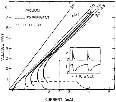
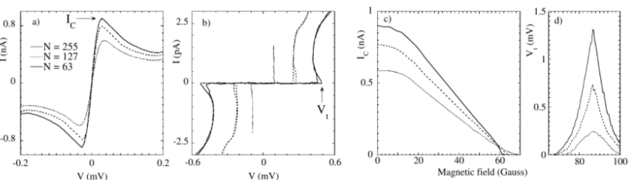
Fig. 2.5: Current-voltage characteristics for tin whisker crystals. Regular step structures are due to successive establishment of phase-slip centers. ∆T = T

− T (from [19])

In 2D films the resistive regions do not consist of phase slip centers, they consist of phase slip lines (PSL), where vortices flow in so called vortex rivers traversing the microbridge vertical to the applied current [50, 51, 52]. The IV characteristics for 2D films behave like for PSCs.

As each PSC makes the filament more resistive, for higher bias-currents dissipation heats up the sample significantly. In Ref. [49] a simple model for self-heating in super- conducting microbridges is presented. Two ways of heat conduction from disipative regions in the microbridge are concerned: Thermal heat conduction within the film to the leads which are at a bath-temperature T

and surface heat transfer from the film to the substrate in which the phonons have a temperature of T

, too. Obviously, due to the longest possible distance to the leads and the most inefficient heat transfer to those, the normal region (“hotspot”) starts to develop from the middle of the bridge.

The model makes several drastic assumptions for simplification. The bridge has a

length L, width w and thickness d with a normal region of length 2x

and resistivity

ρ placed in the center of the bridge. K

is the thermal conductivity in the normal-

conducting and superconducting regions, respectively, and is taken to be temperature

independent. α is the total heat-transfer coefficient per unit area of film for the heat-

transfer between superconducting film and substrate and is taken to be temperature

independent, too. The combination of heat conduction within the film to the leads and

from the film to the substrate leads to a characteristic thermal healing length η

, for

the normalconducting/superconducting regions respectively, given by η

=

K

d α

(2.52) Typical thermal healing length were found to be around 5 µm.

Fig. 2.6: Temperature distributions for a series of hotspot sizes in one-half of a long micro- bridge (L/η

= 11) with the assumption T = T

at the end of the film. The temperature distributions in the other half are axis-symmetrically to the center the same. The dots indicate the normalconducting/superconducting interface with T (±x

) = T

. (from [49])

For long bridges where the length of the bridges is much longer than the healing length η, the temperature distribution T (x) must satisfy the heat-flow equations

−K

d

T dx

+ α

d (T − T

) = I

W d

ρ (|x| < x

) (2.53)

−K

d

T dx

+ α

d (T − T

) =0 (|x| < x

) (2.54)

with I the current through the bridge and x = 0 at the middle of the bridge. The

boundary condition at the leads is T (±

L) = T

which includes the assumption that

the leads cool the boundary to the film perfectly to the bath temperature T

. At the

normalconducting/superconducting interface x

, T and K(dT /dc) have to match with

the boundary condition T (±x

) = T

. The temperature distribution is then given by T

(x) = T

+ (T

− T

)

K

K

coth x

η

× coth

2

L η

− x

η

(

1 − cosh x

η

cosh x

η

) (|x| < x

) (2.55)

T

(x) = T

+ (T

− T

)

sinh

2

L η

− x

η

sinh

2

L η

− x

η

(|x| > x

) (2.56) This self-consistent solution requires a current depending on the position of the super- conducting/normalconducting interface

I(x

) =

αW

d(T

− T

) ρ

"

1 + K

K

coth x

η

coth

2

η

− x

η

#

(2.57) and by Ohm’s law the sample dimensions and the normal state resistivity give the voltage

V (x

) = 2x

ρ

W d · I(x

) (2.58)

The temperature distributions for a series of hotspot sizes for a sample with L/η = 11 with the assumption η

= η

is displayed in Fig. 2.6. IV characteristics for several values of L/η, again with η

= η

, are shown in Fig. 2.7. R

= ρL/W d is the normal state resistance of the bridge. The model contains a characteristic current scale

I

=

αW

d(T

− T

) ρ

(2.59) which is the minimum current to generate a normalconducting hot-spot beglecting the heat conduction within the film.

As can be seen in Fig. 2.7, for long microbridges with L x

η the IV ap-

proaches a constant minimum current at I = (1 + K

/K

)

I

. A scheme of a long

superconducting microstrip with a normalconducting hotspot placed in the center of

the strip is displayed as an inset of Fig. 2.7. Experimental data of IV characteristics

for a 42 µm long and 3 µm wide microstrip is shown in Fig. 2.8. The dotted line,

which corresponds to the hotspot theory for long microbridges, resembles the mea-

sured data (solid and dashed lines) quite well. The theoretical parameters L, W, d, T

and T

are independently measured, ρ was estimated from the normal resistance of

the bridge, K

is estimated by the Wiedemann-Franz law for thermal conductivity

with K

=

π

(k

/e)

T ρ

and K

is taken to be a bit less than K

. Despite the

surface heat-transfer coefficient α is assumed to be constant within the hotspot theory,

it is the only fitting parameter which is varied for various bath temperatures. The

coefficient α in the hotspot theory can be regarded as a mean heat-transfer coefficient

across the bridge for a set bath temperature T

. It is found that current and voltage scaling parameters are proportional to (T

− T

)

, as expected from the theory.

Fig. 2.7: Theoretical IV characteristics for differently long microbridges. Current and voltage are calculated with Eqs. 2.57 and 2.58 respectively. (from [49])

A guidline for fitting is given: ρ adjusts the voltage scale, α/ρ adjusts the minimum current. K

/α and K

/α (and consequently η

and η

) adjust the curvature above and below the region of minimum current, respectively. For all the measured curves in [49] α was in the range 1.0 − 3.5 W/cm

K for glass and saphire substrates and samples which were in vaccum or immersed in a normal helium bath. Though α was taken to be a average coefficient across the bridge within the theory of the hotspot-model, it increases rapidly with increasing bath temperature T

.

A close look at the low-bias regime of the IV characteristics in Fig. 2.8 reveals a behaviour that is not expected from the hotspot theory. Most distinct this feature can be seen for 3.4 K. When the current exceeds the critical current I

, it does not switch immediately along the load line to the current predicted by the hotspot theory.

Instead, circuit-controlled relaxation oscillations occur.

Vernon and Pedersen [53] observed these relaxation oscillations while investigating Josephson junctions. They gave a simple explanation considering a Josephson junc- tion embedded in an external circuit consisting of a dc source with voltage V

in series with a resistor and an inductor. For a small bias-voltage (V

∆/(2e), with ∆ the superconducting energy gap) across the junction, a supercurrent gets accelerated with a time constant that is determined by the external circuit. When the current which is defined by the series resistor exceeds I

, the voltage across the junction jumps to

∆/(2e). The current hence is reduced below I

according to circuit-dependent time

scales. The repetition frequency raises with increasing bias-voltage with a maximum at a voltage of ∆/(2e).

Experimentally, a switching from a plateau-shaped relaxation oscillation region to a zero current region in the IV characteristics was observed, as expected for a small Josephson junction without quasiparticle tunneling below the gap energy of the junc- tion. For superconducting microbridges this switching occurs along the load line resis- tance to the current predicted by the hotspot theory. The waveform of the oscillating voltage and current due to relaxation oscillations is shown in the inset of Fig. 2.8.

Fig. 2.8: Experimentally obtained voltage-biased IV characteristics of a long tin microbridge measured at different bath temperatures T

. The solid and dashed curves are measured data, the dotted curves are based on the hotspot theory for long microbridges. The inset shows the time-evolution of voltage and current across the bridge which correspond to curcuit-controlled relaxation oscillations. (from [49])

The load line in the IV characteristics represents the response of the linear cir-

cuit, that is combined with a non-linear system. In the case here, the linear cir-

cuit is comprised by the series resistor and the superconducting bridge is the non-

linear system. A IV curve for a superconducting niobium nitride film is shown in

Fig. 2.9 from Ref. [54]. The measurement is voltage-biased with a series resistor of

R

= 10 Ω. The corresponding load line is indicated by the dashed red line with a

slope of V . / I. = −R

= −10 Ω. When the critical current I

is exceeded according to

a dc bias voltage V = R

· I

, the current not immediately drops to the relaxation

oscillation plateau, the maximum negative slope in the IV characteristics is deter-

mined by the slope of V . / I. = −R

= −10 Ω. The dashed blue line indicates a load line

originating from a series resistor of R

= 100 Ω. When the critical current is exceeded

under the R

= 100 Ω configuration, the IV curve switches across the load line with

a slope of V . / I. = −R

= −100 Ω to the hotspot plateau. The relaxation oscillation

plateau is not visible in this configuration.

Fig. 2.9: Experimentally obtained voltage-biased IV characteristics of a long microbridge measured at different bath temperatures T

. The solid and dashed curves are measured data, the dotted curves are based on the hotspot theory for long microbridges. The inset shows the time-evolution of voltage and current across the bridge which correspond to curcuit-controlled relaxation oscillations. (from [49])

In niobium nitride (NbN) extensive studies of phase slippages and the evolution of

a normalconducting hotspot were pursued (see e.g. [55]), also because the formation

of the hotspot in NbN can be used for single-photon detection in so called hot electron

bolometers [56, 57]

2.3 Superconductor-insulator transition

For a review about the superconductor-insulator transition read Refs. [58, 59, 60].

2.3.1 Two-dimensional superconducting systems under the influence of disorder

(a) (b)

Fig. 2.10: (a) Evolution of the temperature dependence of the resistance of amorphous Bismuth films deposited onto a Germanium layer. The R(T ) curves shown correspond to film thicknesses ranging from 4.36 to 74.27 nm (from [61]) (b) SIT for a series of TiN films with different resistances at room temperature, which was tuned by soft plasma etching.

(from [62])

The preceding sections of this work shed light on the theory of superconductivity and resistive mechanisms in superconductors. These resistive mechanisms raise the resis- tivity of superconducting samples maximally to about G

= 81 kΩ which is connected to k

l = 1. But for sufficiently disordered 2D films, the resistance increases with de- creasing temperature, contrary to what is expected for a superconducting sample. This phenomenon in called the disorder-driven superconductor insulator transition (D-SIT).

In 1989, Haviland et al. [61] first noticed that Bismuth films grown on Germanium

undergo a disorder-driven SIT (Fig. 2.10a). Since then, the D-SIT has been observed

in amorphous (e.g. indium oxide [63]), polycristalline (TiN) (Fig. 2.10b [62]), granular (lead grains [64]) and also high-T

superconductors [65, 66].

The question how the drop of resistance at low temperatures disappears with increas- ing disorder is still strongly discussed. Anderson showed that nonmagnetic impurities do not affect the superconducting transition temperature [67], but for strong enough disorder Anderson localization of electrons develops, forming a rather than a metal insulating state. Then a superconducting state can not be established, even in the presence of an attractive electron-electron interaction [68].

Finkel’stein [69] estimated the suppression of the superconducting order parameter by disorder, based on a perturbative microscopic description of homogeneously disor- dered systems under consideration of the competition between attractive and repulsive electron-electron interactions in the presence of disorder. The repulsive Coulomb in- teraction increases as disorder increases due to a reduced electron mobility caused by impurity scattering. Finkel’stein calculated the suppression of the critical temperature T

relative to the superconducting transition temperature in the bulk T

with the sheet resistance at room temperature R

taken as a measure for disorder in thin films:

T

T

= exp

− 1 γ

"

1 + (t

/2)

γ

− t

/4

·

1 − (t

/2)

γ

− t

/4

#

(2.60) where γ

= 1/ ln(k

T

τ / ~ ) < 0 and t

= (e

/2π

~ )R

= G

R

. For TiN it has been found that in the vicinity of the SIT Eq. 2.60 holds perfectly [70, 6] despite the predicted strong mesoscopic fluctuations which may develop in the critical region and lead to deviations from Eq. 2.60 [71]. For sufficiently high disorder the Coulomb repulsion between electrons is strong enough to break down Cooper pairing and destroy superconductivity.

In such a fermionic scenario the arising Anderson localization of electrons leads to

an insulating state. This at first sight offers a plausible explanation of the SIT, but the

degree of disorder to balance Coulomb repulsion and Cooper pairing (T

→ 0), is not

sufficient to localize normal carriers. This would result in a SIT with an intermediate

metallic state between the superconducting and insulating states. As can be seen

in Fig. 2.10b this obviously is not always the case, a sharp transition between the

superconducting and insulating regimes is observed.