Flavor effects on leptogenesis predictions

Flavor effects on leptogenesis predictions

Steve Blanchet and Pasquale Di Bari

Max-Planck-Institut f¨ ur Physik (Werner-Heisenberg-Institut) F¨ohringer Ring 6, 80805 M¨ unchen

August 11, 2006

Abstract

We show that flavor effects in leptogenesis reduce the region of the see-saw

parameter space where the final predictions do not depend on the initial conditions,

the strong wash-out regime. In this case the lowest bounds holding on the lightest

right-handed (RH) neutrino mass and on the reheating temperature for hierarchical

heavy neutrinos do not get relaxed compared to the usual ones in the one-flavor

approximation,

(T

)

3 (1.5)

10

GeV. Flavor effects can however relax

down to these minimal values the lower bounds holding for fixed large values of the

decay parameter

. We discuss a relevant definite example showing that, when the

known information on the neutrino mixing matrix is employed, the lower bounds

for

10 are relaxed by a factor 2-3 for light hierarchical neutrinos, without

any dependence on

and on possible phases. On the other hand, going beyond

the limit of light hierarchical neutrinos and taking into account Majorana phases,

the lower bounds can be relaxed by one order of magnitude. Therefore, Majorana

phases can play an important role in leptogenesis when flavor effects are included.

1 Introduction

The see-saw mechanism [1] is a simple and elegant way to understand neutrino masses and their lightness compared to all other fermions. At the same time, with leptogenesis [2], the see-saw offers an attractive model to explain the matter-antimatter asymmetry of the Universe. The asymmetry is produced in the decays of the very heavy RH neutrinos, necessary for the see-saw mechanism to work, generating a B − L asymmetry in the form of a lepton asymmetry partly converted into a baryon asymmetry by sphaleron processes if temperatures are larger than about 100 GeV [3].

Calculations have been typically performed within a one-flavor approximation, assum- ing that the final total B − L asymmetry is not sensitive to the dynamics of the individual B/3 − L

asymmetries. In this case it has been noticed [4, 5] that current neutrino mixing data favor leptogenesis to lie in a region of the parameter space where thermal equilibrium sets up prior to the freeze-out of the final asymmetry and therefore, if the temperature of the early Universe is large enough, the final asymmetry does not depend on the initial conditions.

For a hierarchical heavy neutrino spectrum, successful leptogenesis requires the mass of the lightest [6] or of the next-to-lightest [7] RH neutrino to be large enough, if the RH neutrino production occurs through scatterings in the thermal plasma. In this case there is also an associated lower bound on the initial temperature of the radiation-dominated regime in the early Universe, to be identified with the reheating temperature, T

, within inflation. Being independent of the initial conditions, these bounds are particularly rele- vant, since they appear as an intrinsic feature of leptogenesis.

Recently it has been pointed out that flavor effects can strongly modify leptogenesis

predictions [8, 9, 10, 11, 12, 13, 14]. In this work we investigate how the dependence

on the initial conditions and the lower bounds on the RH neutrino masses and on the

reheating temperature are modified when flavor effects are included. The calculations are

presented within the hierarchical limit for the spectrum of the heavy neutrino masses, and

more specifically in the lightest RH neutrino dominated scenario (N

DS), where the final

asymmetry is dominantly produced by the lightest RH neutrino decays. In the second

Section we set up the notation and the kinetic equations. In the third Section we analyze

how flavor effects modify the dependence on the initial conditions. In the fourth Section

we perform explicit calculations for a specific but significant example. In the Appendix

we discuss the role of ∆L = 1 scatterings, showing how they introduce just a correction

to the results.

2 General set-up

Adding to the Standard Model Lagrangian three RH neutrinos with a Yukawa coupling matrix h and a Majorana mass matrix M , a neutrino Dirac mass matrix m

= h v is generated, after electro-weak symmetry breaking, by the vev v of the Higgs boson. For M ≫ m

, the neutrino mass spectrum splits into 3 heavy Majorana states N

, N

and N

with masses M

≤ M

≤ M

, almost coinciding with the eigenvalues of M , and 3 light Majorana states with masses m

≤ m

≤ m

, corresponding to the eigenvalues of the neutrino mass matrix given by the see-saw formula,

m

= − m

1

M m

. (1)

Neutrino mixing experiments measure two mass-squared differences. In normal (inverted) neutrino schemes, one has

m

− m

= ∆m

(∆m

) , (2) m

− m

= ∆m

(∆m

− ∆m

) . (3) For m

≫ m

≡ p

∆m

+ ∆m

≃ 0.05 eV, one has a quasi-degenerate spectrum with m

≃ m

≃ m

, whereas for m

≪ m

≡ p

∆m

≃ 0.009 eV one has a fully hierarchical (normal or inverted) spectrum.

A lepton asymmetry can be generated from the decays of the heavy neutrinos into leptons and Higgs bosons and partly converted into a baryon asymmetry by the sphaleron (B − L conserving) processes at temperatures higher than about 100 GeV.

Below some temperature T

, muon and tauon charged lepton Yukawa interactions

become strong enough to break the coherent evolution of the lepton doublets quantum

states, the | l

i ’s, produced in RH neutrino decays and make them collapse into one of

the three-flavor eigenstates, the | l

i ’s, with probability |h l

| l

i|

. There is quite a large

uncertainty on the value of T

and two different results have been quoted by different

groups. One group [12] finds T

≃ 10

GeV, while other groups [8, 13] find T

≃

10

GeV. For temperatures 10

GeV ≃ T

& T & T

, only tauon charged lepton

Yukawa interactions are in equilibrium and in this case the quantum state is projected

on a two-flavor basis, where the eigenstates are given by the tauon flavor and by a linear

combination of muon and electron flavors. In the following we will always assume to

work in the three-flavor regime, with T . T

≃ 10

GeV. This is the most conservative

assumption since the deviations from the one-flavor approximation are in general even

larger than in a two-flavor regime. However, in specific contexts, we will also give the

results calculated in the two-flavor regime.

Flavor effects play a double role in leptogenesis. A first effect is that the wash-out is reduced. This happens because only the projections of the flavor lepton eigenstates onto the | l

i ’s interact with the Higgs. This effect can be accounted for introducing the flavor projectors [12]

P

= |h l

| l

i|

= Γ

Γ

, (4)

P

= |h ¯ l

| l

i|

= Γ

Γ

, (i = 1, 2, 3; α = e, µ, τ ) (5) where Γ

is the partial decay rate of the process N

→ l

+ H

and Γ

= P

α

Γ

is the total decay rate, such that P

α

P

= 1. Analogously Γ

is the partial decay rate of the process N

→ ¯ l

+ H with Γ

= P

α

Γ

, such that P

α

P

= 1.

A rigorous description of the asymmetry evolution has then to be performed in terms of the individual flavor asymmetries ∆

≡ B/3 − L

rather than in terms of the total asymmetry N

= P

α

N

, as usually done in the one-flavor approximation. The con- tribution of each decay to the N

’s is determined by the individual flavor CP asymmetry, defined as

ε

≡ − Γ

− Γ

Γ

+ Γ

. (6)

A second role played by flavor effects arises because the state | ¯ l

i is not the CP conjugated state of | l

i [12] and this yields an additional source of CP violation. This can be described in terms of the projector differences [12]

∆P

≡ P

− P ¯

, (7)

obeying P

α

∆P

= 0. Indeed writing P

= P

+ ∆P

/2 and P

= P

− ∆P

/2, where the P

≡ (P

+ P

)/2 are the tree level contributions to the projectors, one can see that

ε

= ε

P

+ ∆ P

2 , (8)

where the total CP asymmetries ε

≡ P

α

ε

. The three flavored CP asymmetries can be calculated using [15]

ε

= 1 8 π (h

h)

X

j6=i

Im

h

h

3 2 √ x

(h

h)

+ 1 x

(h

h)

. (9)

In the last years there has been an intense study of the relevant processes in leptogenesis

[16, 17, 18]. For our purposes it will be enough to describe the evolution of the asymmetries

just in terms of decays and inverse decays (after subtraction of the real intermediate

state contribution from ∆L = 2 processes) neglecting scatterings, spectator processes and thermal effects. In the Appendix we will discuss and justify this approximation. We will also neglect off-shell ∆L = 2 and ∆L = 0 processes since these are relevant only at higher temperatures. The kinetic equations, using z ≡ M

/T as the independent variable, are then given by [12, 19]

dN

dz = − D

(N

− N

) (10) dN

dz = X

i

ε

D

(N

− N

) − P

X

i

W

N

,

where the N

’s and the N

’s are the abundances per number of N

’s in ultra-relativistic thermal equilibrium. The equilibrium abundances are given by N

= z

K

(z

)/2, where we indicate with K

(z

) the modified Bessel functions. Introducing the decay parameters K

≡ e Γ

/H (T = M

), the ratios of the total decay widths to the expansion rate at T = M

, the decay terms D

can be written like [5]

D

≡ Γ

H z = K

x

z 1

γ

, (11)

where the h 1/γ

i ’s are the thermally averaged dilation factors and are given by the ratios K

(z

)/ K

(z

). Finally, the inverse decays wash-out terms are given by

W

(z) = 1

4 K

√ x

K

(z

) z

, (12) where x

≡ (M

/M

)

. The evolution of the N

’s can be worked out in an integral form,

N

(z) = N

e

Rz

zin dz^′W_i^ID(z^′)

+ X

i

ε

κ

(z) , (13) with the 9 efficiency factors given by

κ

(z; K

, P

) = − Z

z_in

dz

dN

dz

e

. (14) The total final B − L asymmetry is then given by N

= P

α

N

. Finally from this, assuming a standard thermal history and accounting for the sphaleron converting coefficient a

∼ 1/3, the final baryon-to-photon number ratio can be calculated as

η

= a

N

N

≃ 0.96 × 10

N

, (15) to be compared with the measured value [20]

η

= (6.3 ± 0.3) × 10

. (16)

Notice that the efficiency factors depend only on the P

but not on the differences ∆P

. Notice also that in the two-flavor regime, for T

& T & T

, the procedure for the calculation of the final asymmetry gets easily modified. The kinetic equations for the individual electron and muon asymmetries have to be replaced by one kinetic equation for the sum, N

≡ N

+N

, where the individual flavored CP asymmetries and projectors have also to be replaced by the their sum, namely ε

≡ ε

+ε

and P

≡ P

+P

[14].

The calculation is therefore somehow intermediate between the one-flavor approximation and the three-flavor regime.

The final asymmetry depends in general on all the unmeasured 14 see-saw parameters.

A useful parametrization is provided by the orthogonal see-saw matrix Ω [21], in terms of which one has m

= U √

D

Ω √

D

. In this way the decay parameters can be expressed as

K

= X

j

m

m

| Ω

| , (17) where m

≃ 10

eV is the equilibrium neutrino mass, and the tree level projectors as

P

= | P

j

√ m

U

Ω

|

P

j

m

| Ω

| . (18)

It will also prove useful to introduce the quantities K

≡ P

K

. The orthogonal matrix can in turn be decomposed as

Ω = R

(ω

) R

(ω

) R

(ω

) , (19) such to be parameterized in terms of three complex numbers, ω

, ω

and ω

, deter- mining the rotations in the planes 12, 13 and 23 respectively. In this way one has η

= η

(m

, U, M

, ω

). It is interesting that including flavor effects there is a poten- tial dependence of the final asymmetry also on the unknown parameters contained in the PMNS mixing matrix U [9, 12].

In the following we will assume a hierarchical heavy neutrino spectrum with M

, M

≫ M

. We will moreover assume no rotation in the plane 23, i.e. R

= 1. Under these

1Just in passing, we notice that it is straightforward to generalize, including flavor effects, a result obtained in [19] for the efficiency factors in the degenerate limit, obtained for (M3−M1)/M1 . 0.1, within the one-flavor approximation and forKⁱ ≫1, for alli. Indeed, in this case one can approximate dNi/dz^′ ≃dNi^eq/dz^′ in the Eq. (14) obtaining that κ^fiα ≃κ(Kα), where Kα ≡P

i Kiα. The function κ(x) is defined in the Eq. (25) and it approximates κ^f1α in the hierarchical limit when x = K1α. In the degenerate limit one has then just to replace K1α with the sumKα. Like in the hierarchical limit, the number of efficiency factors to be calculated reduces from 9 to 3, one for each flavor. If instead of a full degeneracy, one has just a partial degeneracy, with M3 ≫ M2 ≃ M1, then simply one has κ^f3α≪κ^f1α≃κ^f2α≃κ(K1α+K2α).

conditions both the total CP asymmetries ε

and ε

and the flavored CP asymmetries ε

and ε

, associated to the decays of the two heavier RH neutrinos, are suppressed

∼ (M

/M

)

. The dominant contribution to the final asymmetry comes then from the lightest RH neutrino and

N

≃ X

α

ε

κ

. (20)

It will prove important for our discussion that the CP asymmetries cannot be arbitrarily large. The total CP asymmetry is indeed upper bounded by [22, 6, 4]

ε

≤ ε(M

) β

f (m

, K

), (21) where ε(M

) ≡ 3 M

m

/(16 π v

), β

≡ m

/(m

+ m

) and 0 ≤ f (m

, m e

) ≤ 1 is a function that vanishes for K

= m

/m

and tends to unity for m

/(m

K

) → 0. On the other hand each individual flavor asymmetry ε

is bounded by [14]

| ε

| < ε(M

) q

P

m

m

max

[ | U

| ] (22) and therefore while the total CP asymmetry is suppressed when m

increases, the single flavor asymmetries can be enhanced. The existence of an upper bound on the quantity r

≡ ε

/ε(M

) independent of M

, imply, as in the case of one-flavor approximation, the existence of a lower bound on M

given by

M

≥ M

≃ N

a

16 π v

3

η

/m

κ

(K

) ξ

(K

) ≥ 4.2 × 10

GeV

κ

(K

) ξ

(K

) (at 3 σ C.L.) , (23) where we indicated with κ

(K

) the efficiency factor in the usual one-flavor approximation, corresponding to κ

with P

= 1. We also defined ξ

≡ P

α

ξ

, with ξ

≡ r

κ

(K

)

κ

(K

) . (24)

This quantity represents the deviation introduced by flavor effects compared to the one- flavor approximation in the hierarchical light neutrino case. We could then use r

≤ p P

m

/m

to maximize ξ

. Notice however that first, because of the bound on the total asymmetry, the r

’s cannot be simultaneously equal to p

P

and second in ξ

there are sign cancellations. Therefore, the bound (23) is more restrictive than this possible estimation and we prefer to keep it in this form, specifying ξ

in particular situations.

As usual, the lower bound on M

imply also an associated lower bound on T

&

M

/(z

(K

) − 2).

3 Dependence on the initial conditions

From the Eq. (14), extending an analytic procedure derived within the one-flavor ap- proximation [5], one can obtain simple expressions for the κ

’s. In the case of an initial thermal abundance (N

= 1) one has

κ

≃ κ(K

) ≡ 2 K

z

(K

)

1 − e

, (25)

where

z

(K

) ≃ 2 + 4 K

e

. (26) Notice that in the particularly relevant range 5 . K

. 100 this expression is well approximated by a power law [23],

κ

≃ 0.5

K

. (27)

In the case of initial vanishing abundance (N

= 0) one has to take into account two different contributions, a negative and a positive one,

κ

= κ

(K

, P

) + κ

(K

, P

) . (28) The negative contribution arises from a first stage when N

≤ N

, for z ≤ z

, and is given approximately by

κ

(K

, P

) ≃ − 2

P

e

e

1α0

2 NN1(zeq)

− 1

. (29)

The N

abundance at z

is well approximated by

N

(z

) ≃ N (K) ≡ N (K

) 1 + p

N (K

)

, (30) interpolating between the limit K

≫ 1, where z

≪ 1 and N

(z

) = 1, and the limit K

≪ 1, where z

≫ 1 and N

(z

) = N (K

) ≡ 3πK

/4. The positive contribution arises from a second stage when N

≥ N

, for z ≥ z

, and is approximately given by

κ

(K

, P

) ≃ 2 z

(K

) K

1 − e

K1α zB(K1α)NN1(zeq) 2

. (31)

Notice, from the Eq. (30), how N

(z

) is still regulated by K

and this because the RH

neutrino production is not affected by flavor effects, contrarily to the wash-out, which is

reduced and is regulated by K

.

These analytic expressions make transparent the two conditions to have independence on the initial conditions. The first is the thermalization of the N

abundance, such that, for an arbitrary initial abundance one has N

(z

) = 1. The second is that the asymmetry produced during the non-thermal stage, for z ≤ z

, has to be efficiently washed out such that κ

≪ κ

. They are both realized for large values of K

≫ 1.

More quantitatively, it is useful to introduce a value K

such that, for K

≥ K

, the final asymmetry calculated for initial thermal abundance differs from that one calculated for vanishing initial abundance by less than some quantity δ. This can be used as a precise definition of the strong wash-out regime. Let us consider some particular cases, showing how flavor effects tend to enlarge the domain of the weak wash-out at the expense of the strong wash-out regime.

3.1 Alignment

The simplest situation is the alignment case, realized when the N

’s decay just into one- flavor α, such that P

= P

= 1 and P

= P

= 0, implying ε

= ε

. Notice that we do not have to worry about the fact that the lightest RH neutrino inverse decays might not be able to wash-out the asymmetry generated from the decays of the two heavier ones, since we are assuming negligible ε

and ε

anyway. In this case the general set of kinetic equations (10) reduces to the usual one-flavor case and all results coincide with those in the one-flavor approximation [12]. In particular one has N

= ε

κ

.

In the considered case of alignment, one obtains K

≃ 3.5 for δ = 0.1, as shown in Fig. 1. The value of K

plays a relevant role since only for K

& K

one has leptogenesis predictions on the final baryon asymmetry resulting from a self-contained set of assump- tions. On the other hand for K

. K

leptogenesis has to be complemented with a model for the initial conditions.

In addition to that, one has to say that in the weak wash-out regime the calculation of the final asymmetry requires a precise description of the RH neutrino production, potentially sensitive to many poorly known effects. It is then interesting that current neutrino mixing data favor K

to be in the range K

∼ 10 . K

. K

∼ 50 [4, 5, 7], where one can have a mild wash-out assuring full independence of the initial condition, as one can see in Fig. 1, but still successful leptogenesis. In this case one can place constraints on the see-saw parameters not depending on specific assumptions for the initial conditions and with reduced theoretical uncertainties.

Since one has ξ

= 1, the general lower bound on M

(see Eq. (23)), like all other

quantities, becomes the usual lower bound holding in the one-flavor approximation. In

10^-1 10⁰ 10¹ 10² 10³

10^-1 10⁰ 10¹ 10² 10³

10^-5 10^-4 10^-3 10^-2 10^-1 10⁰

10^-5 10^-4 10^-3 10^-2 10^-1 10⁰

K_atm K_sol

N

N₁

=0 N

N₁

=1

κ

K

K

-1 10⁰ 10¹ 10² 10³

10^-1 10⁰ 10¹ 10² 10³

10⁸ 10⁹ 10¹⁰ 10¹¹ 10¹²

10⁸ 10⁹ 10¹⁰ 10¹¹ 10¹²

K

3x10⁹

K_atm K_sol

N

N₁

=1

K

N

N₁

=0

GeV

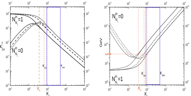
Figure 1: Efficiency factor (left panel) and lower bounds on M

(right panel) in the alignment (solid), in the semi-democratic (dashed lines) and in the democratic (short- dashed) cases.

the right panel of Fig. 1 we have plotted it both for N

= 1 and N

= 0. One can see that the κ

dependence on the initial conditions translates into a dependence of M

. The lowest model-independent values are then obtained for K

= K

≃ 3.5 and are given by

M

& 3 × 10

GeV and T

& 1.5 × 10

GeV . (32)

3.2 Democratic and semi-democratic cases

Let us now consider another possibility where P

= ¯ P

= 1/3 for any α and consequently

∆ P

= 0. From the Eq.’s (14) it follows that the three κ

, like also the three ε

, are all equal and thus the Eq. (20) simplifies into N

= ε

κ

, as in the usual one-flavor approximation. However now the wash-out is reduced by the presence of the projector, such that K

→ P

K

= K

/3. The result is that in the case of an initial thermal abundance the efficiency factor, as a function of K

, is simply shifted. The same happens for vanishing initial abundance in the strong wash-out regime. However, in the weak wash-out regime, there is not a simple shift, since the RH neutrino production is still depending on K

. A plot of κ

is shown in the left panel of Fig. 1 (dashed lines).

One can see how the reduced wash-out increases the value of K

to ∼ 10, approximately

1/P

≃ 3 larger, thus compensating almost exactly the wash-out reduction by a factor

∼ 3

(cf. (27)).

In this way the lowest bounds on M

in the strong wash-out regime, at K

= K

, are almost unchanged. On the other hand for a given value of K

≫ K

, the lower bounds get approximately relaxed by a factor 3 [13]. The lower bounds for the democratic case are shown in the right panel of Fig. 1 (dashed lines).

The semi-democratic case is an intermediate case between the democratic and the alignment. It is obtained when one projector vanishes, for example P

= 0, and the other two are one half and in this case K

∼ 7. The corresponding plot of the efficiency factor and of the lower bound on M

are also shown in Fig. 1 (short-dashed lines). These results also apply for T & T

in the two flavor regime, when the two projectors are equal, namely P

= P

= 1/2.

3.3 One-flavor dominance

There is another potentially interesting situation that motivates an extension of the pre- vious results to arbitrarily small values of P

. This occurs when the final asymmetry is dominated by one-flavor α and the Eq. (20) can be further simplified into

N

≃ ε

κ

, (33) analogously to the alignment case but with P

≪ 1. Notice that this cannot happen due to a dominance of one of the CP asymmetries, for example with ε

being close to its maximum value, Eq. (22), much larger than the other two strongly suppressed, simply because one has P

α

∆P

= 0. One has then to imagine a situation where the CP asymmetry ε

is comparable to the sum of the other two but K

≫ K

& 1 such that κ

≫ κ

. The dominance is then a result of the much weaker wash-out.

The analysis of the dependence on the initial conditions can then be again performed as in the previous cases calculating the value of K

for any value of P

. The result is shown in Fig. 2. The alignment case corresponds to P

= 1, the semi-democratic case to P

= 1/2 and the democratic case to P

= 1/3. Notice that the result is very close to the simple estimation K

(P

) = K

(1)/P

, that would follow if κ

were just depending on K

. In Fig. 3 we have plotted the values of the lower bounds on M

and T

for light hierarchical neutrinos, implying m

= m

in the Eq. (22). These can be obtained plugging ξ

= p

P

κ

(K

)/κ

(K

) ≤ 1 in the Eq. (23). They correspond to the lowest values in the strong wash-out regime, when K

≥ K

.

There are two possible ways to look at the results. As a function of P

they get

more stringent when P

decreases. This is clearly visible in the left panel of Fig. 3. In

10^-2 10^-1 10⁰

10^-2 10^-1 10⁰

10⁰ 10¹ 10² 10³

10⁰ 10¹ 10² 10³

P

1α

K

Figure 2: Value of K

, defining the strong wash-out regime for δ = 10% (solid line) and δ = 50% (dashed line).

particular, one can conclude that flavor effects cannot help to alleviate the conflict of the leptogenesis lower bound on the reheating temperature with the gravitino problem upper bound. On the other hand, flavor effects can relax the lower bound for fixed values of K

≫ 1. Indeed, for each value K

≫ 1, one can choose P

= K

(P

= 1)/K

such that K

= K

(P

), thus obtaining the highest possible relaxation in the strong wash-out regime. The result is shown in the right panel of Fig. 3. It is important to say that this relaxation is potential. A direct inspection is indeed necessary to determine whether it is really possible to achieve at the same time not only small values of P

, but also a ε

that is not suppressed compared to ε

.

In the next Section, we will consider a specific example that will illustrate what we have discussed on general grounds. At the same time it will help to understand which are realistic values for the projectors and their differences, given a specific set of see-saw parameters and using the information on neutrino mixing matrix we have from low-energy experiments.

4 A specific example

The previous results have been obtained assuming no restrictions on the projectors. More-

over, in the one-flavor dominance case, where there can be a relevant relaxation of the

usual lower bounds holding in the one-flavor approximation, we have assumed that the

10^-2 10^-1 10⁰

10^-2 10^-1 10⁰

10⁹ 10¹⁰ 10¹¹

10⁹ 10¹⁰ 10¹¹

GeV

M

1

T

reh

P

1α

10⁰ 10¹ 10²

10⁰ 10¹ 10²

10⁹ 10¹⁰ 10¹¹

10⁹ 10¹⁰ 10¹¹

GeV

M

1

T

reh

K

Figure 3: Lower bounds on M

and T

calculated choosing P

= K

(P

= 1)/K

such that K

= K

(P

) (thick lines) and compared with the usual bounds for P

= 1 (thin lines). In the left panel they are plotted as a function of P

, while in the right panel as a function of K

.

upper bound on ε

, see Eq. (22), is saturated independently of the value of the projector.

This assumption does not take into account that the values of the projectors depend on the different see-saw parameters, in particular on the neutrino mixing parameters, and that severe restrictions could apply. Let us show a definite example considering a particular case for the orthogonal matrix,

Ω = R

=



 

p 1 − ω

0 − ω

0 1 0

ω

0 p

1 − ω



  . (34)

This case is particularly meaningful, since it realizes one of the conditions (Ω

= 0) to saturate the bound (21) for ε

that is given by ε

= ε(M

) Y

m

/ m e

, with Y

≡ − Im[ω

] [7]. Moreover the decay parameter is given by

K

= K

| 1 − ω

| + K

| ω

| , (35) where K

≡ m

/m

and K

≡ m

/m

. The expression (18) for the projector gets then specialized as

P

= m

| U

|

| 1 − ω

|

+ m

| U

|

| ω

|

+ 2 √ m

m

Re[U

U

p

1 − ω

ω

]

m

| 1 − ω

| + m

| ω

| , (36)

while, specializing the Eq. (9) for ε

and neglecting the term ∝ x

, one obtains r

= Y

m

m e

| U

|

+ m

m

( | U

|

− | U

|

)

(37) + m

e m

r m

m

m

m

m

+ m

m

Im

ω

q

1 − ω

| 1 − ω

| − | ω

|

Re[U

U

] +

m

− m

m

Re

ω

q

1 − ω

| 1 − ω

| + | ω

|

Im[U

U

]

, where m

/m

= p

1 + m

/m

.

If we first consider the case of fully hierarchical light neutrinos, m

= 0, then P

= ε

ε

= | U

|

and ∆P

2 ε

= 0 . (38)

Neglecting the effect of the running of neutrino parameters from high energy to low energy [24], one can assume that the U matrix can be identified with the PMNS matrix as measured by neutrino mixing experiments. We will adopt the parametrization [25]

U =



 

c

c

s

c

s

e

− s

c

− c

s

s

e

c

c

− s

s

s

e

s

c

s

s

− c

c

s

e

− c

s

− s

c

s

e

c

c



 × diag(e

, e

, 1) , (39) where s

≡ sin θ

, c

≡ cos θ

and where we have used θ

= 0 − 0.17, θ

= π/6 and θ

= π/4. One then finds

P

. 0.03 , P

≃ P

≃ 1/2 . (40) This result implies a situation where the projector on the electron flavor is very small and the associated generated asymmetry as well, while the muon and tauon contributions are equal. Notice that even though there is a non-vanishing extra contribution to the muon and tauon CP asymmetries, they have equal absolute value but opposite sign. Therefore, since the projectors are equal as well, summing the kinetic equations (10) over α, one simply recovers the one-flavor approximation with the wash-out reduced by a factor 1/2.

This is a realization of the semi-democratic case that we were envisaging at the end of 3.2 where K

≃ 7. In this situation flavor effects do not produce large modifications of the usual results, essentially a factor 2 reduction of the wash-out in the strong wash-out regime with a consequent equal relaxation of the lower bounds (see dashed lines in Fig.

1). Notice moreover that the indetermination on T

is not relevant since the result in a

two-flavor regime, for T & T

, would be essentially the same.

0 0.1 0.2 0.3 0.4 0.5 0.6 0.7 0.8

10 100

K₁ e

µ τ

e µ τ

P⁰_1α r_1α

-0.5 0 0.5 1 1.5 2 2.5 3 3.5

10 100

K₁ e µ

τ ξ_1α

ξ₁

10⁹ 10¹⁰ 10¹¹ 10¹²

10 100

K₁

GeV

K_*

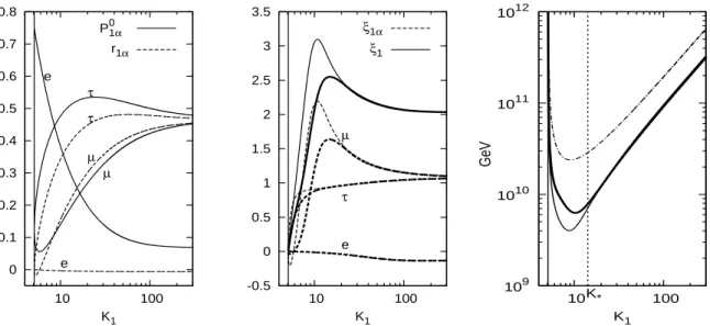
Figure 4: Dependence of different quantities on K

for m

/m

= 0.1 and real U . Left panel: projectors P

and r

; central panel: ξ

and ξ

as defined in Eq. (24) for thermal (thin) and vanishing (thick) initial abundance; right panel: lower bound on M

for thermal (thin solid) and vanishing (thick solid) abundance compared with the one- flavor approximation result (dash-dotted line).

Let us now consider the effect of a non-vanishing but small lightest neutrino mass m

, for example m

= 0.1 m

. In this case the results can also depend on the Majorana and Dirac phases. We will show the results for ω

purely imaginary, the second condition that maximizes the total CP asymmetry if m

≪ m

[7]. Notice that this is not in general the condition that maximizes r

for non-vanishing m

, however we have checked that, allowing for a real part of ω

, one obtains similar bounds within a factor O (1).

We have first considered the case of a real U . The results are only slightly sensitive to a variation of θ

within the experimentally allowed range 0 − 0.17. Therefore, we have set θ

= 0, corresponding to U

= 0, in all the shown examples. In the left panel of Fig. 4 we show the values of the projectors, the P

’s, and of the r

’s as a function of K

. One can notice how, while the electron projector and asymmetry are still strongly suppressed, now a difference between the tauon and the muon projectors and asymmetries arises. On the other hand for K

≫ 100 this difference tends to vanish and the semi-democratic case is recovered again.

In the cental panel we have also plotted the quantities ξ

(cf. (24)) and their sum ξ

,

where we recall that ξ

gives the deviation of the total asymmetry from a calculation in

the one-flavor approximation for hierarchical light neutrinos. One can see how now the

0 0.1 0.2 0.3 0.4 0.5 0.6 0.7 0.8

10 100

K₁ e

µ τ

e µ τ

P⁰_1α r_1α

0 1 2 3 4

10 100

K₁ e

µ

τ ξ_1α

ξ₁

10⁹ 10¹⁰ 10¹¹ 10¹²

10 100

K₁

GeV

K_*

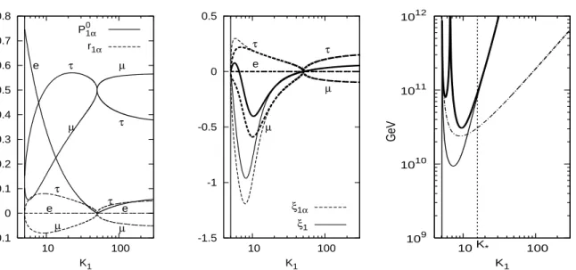
Figure 5: As in the previous figure but with one non vanishing Majorana phase: Φ

= π.

contribution to the total asymmetry from the muon flavor can be twice as large as from the tauon flavor. For K

≫ 100 the semi-democratic case is restored, the two contributions tend to be equal to the one-flavor approximation case and the total final asymmetry is about twice larger. Finally in the right panel we have plotted the lower bound on M

and compared them with the results in the one-flavor approximation (dash-dotted line). At K

≃ 14 the relaxation is maximum, a factor ∼ 3. For K

≫ K

the relaxation is reduced to a factor 2, as in the semi-democratic case.

Let us now study the effect of switching on phases in the U matrix, again for m

= 0.1 m

. The most important effect arises from one of the two Majorana phases, Φ

. In Fig. 5 we have then again plotted, in three panels, the same quantities as in Fig. 4 for Φ

= π. One can see how this further increases the difference between the muon and the tauon contributions and further relaxes the lower bound on M

. The effect is small for the considered value m

/m

= 0.1. However, considering a much larger value while keeping Φ

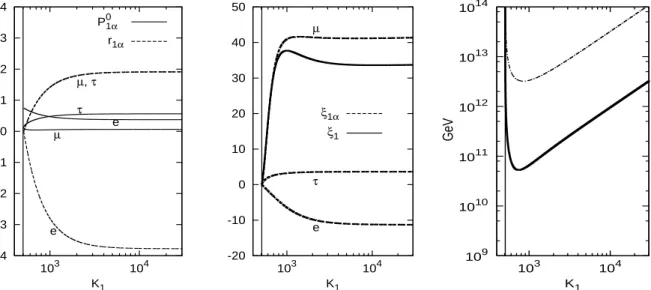
= π, the effect becomes dramatically bigger. In Fig. 6 we have plotted the same quantities as in Fig. 4 and Fig. 5 for m

/m

= 10. In the left panel one can see that now, for K

≫ K

, r

≃ r

≃ 2, much larger than in the previous case.

This means that the dominant contribution to the flavored CP asymmetries comes now

from the ∆P

term. At the same time, very importantly, P

≪ P

and in this way, as

one can see in the central panel, the dominant contribution to ξ

is given by ξ

. This

case thus finally realizes a one-flavor dominance case. The final effect is that the lower

bound on M

is about one and half order of magnitude relaxed compared to the one-flavor

-4 -3 -2 -1 0 1 2 3 4

10³ 10⁴

K₁ e

µ, τ

e τ µ

P⁰_1α r_1α

-20 -10 0 10 20 30 40 50

10³ 10⁴

K₁ e τ µ

ξ_1α ξ₁

10⁹ 10¹⁰ 10¹¹ 10¹² 10¹³ 10¹⁴

10³ 10⁴

K₁

GeV

Figure 6: Same quantities as in the previous two figures but with m

/m

= 10 and one non-vanishing Majorana phase: Φ

= π.

approximation.

In the left panel of Fig. 7 we have summarized the dependence on m

/m

of the lower bound on M

, plotting both the case with zero Majorana phase and the case with Φ

= π. One can see how without Majorana phase there is an increase in the relaxation of the lower bound and of the effect of the phase. In the right panel we have also shown the results in the two-flavor regime for T & T

. There is no remarkable difference but notice that now the dominance occurs in the τ flavor and that the maximum phase effect is for Φ

= − π.

Finally we wanted to study the interesting case of a real orthogonal matrix Ω, implying ε

= 0. If m

= 0 there is practically no produced asymmetry, since the ε

∝ ε

= 0. For a non vanishing m

and a non-real U however the ∆P

6 = 0 and consequently ε

6 = 0. In Fig. 8 we have shown the results for m

/m

= 0.1 and Φ

= π/2. We have again plotted the same quantities as in Fig. 4, 5 and 6 in three different panels. One can see that an asymmetry can be still produced, as emphasized in [12]. However successful leptogenesis is possible only in the weak wash-out regime. In the strong wash-out regime, for values M

. 10 T

. 10

GeV, there is a very small allowed region only for K

≃ 14 ≤ K

. 30.

This somehow means that, at least in the example we are considering and for small m

, flavor effects give a sub-dominant effect.

We can thus draw two remarkable conclusions. The first is that the relaxation of the

lower bounds compared to the one-flavor approximation is only O (1) for m

≪ m