Photoeffect IIA3

IIA3

Modul Atomic/Nuclear Physics

Photo effect

Using different experiments, it was at the end of the last century shown

that electrons can be freed from a metal by irradiating the surface with

light. This process is called photoelectric effect (photo-emission) and the

emitted electrons are photo-electrons. By means of the photon emission,

it is possible that P

’

constant can be determined.

Using different experiments, it was at the end of the last century shown that electrons can be freed from a metal by irradiating the surface with light. This process is calledphotoelectric effect (photo-emission)and the emitted electrons arephoto-electrons. By means of the photon emission, it is possible that PLANCK’Sconstant can be determined.

c

AP, Department of Physics, University of Basel, September 2016

1.1 Preliminary Questions

• Describe the photoelectric effect in their own words.

• Describe exactly how the energy of the photons is measured in the photocell.

• Why did the high-pressure mercury lamp have a (discrete) line spectrum?

1.2 Theory

1.2.1 Photo electrons

Looking for a source of electromagnetic waves was examined H

H

in 1887, with the discharge between two electrodes. He observed that the intensity of the discharge grew when the cathode was irradiated with ultraviolet light. The effect suggested the as- sumption that metal surfaces are irradiated with light, emit electrons. Shortly afterwards, W. H

and somewhat later P. L

could find evidence of electron emission of irradiated surfaces with zinc, potassium, rubidium and sodium.

In a metal, there are many electrons, that more or less move together freely through the crystal lattice. If not for high temperatures, but can not galvanize from the metal because they have too little energy due to the strong C

force to overcome forces at the surface. One possibility to give the electron more energy is to heat the metal. "Steaming" the electrons then from the top face out; they are then called thermal electrons. This type of electron emission (thermal emission) occurs in electron tubes. A second possibility is the field emission. Here, a strong external electric field electron challenges from the metal sucked. The emerging field electrons can be noticed by electric sparks in the air, as in spark plugs.

1.2.2 M

’s Observations

In 1914, A. M

examined the photoelectric effect again with the great care. Figure 1.1 shows a schematic representation of the experimental arrangement: to great confusion of his contemporaries, his observations were not explained with the classical rectangular wave theory of light (electrodynamics):

incoming photons

electrons

photo-cathode collector / anode

V₊

light current

Figure 1.1: Schematic representation of M

’

Setup

3

• Emission of electrons (i.e., the photoelectric current in the electrode j) grows, although, with the intensity of the incident on the metal surface light radiation; the kinetic en- ergy of the emitted electrons proves irrespective. After electrodynamics, the intensity I increases with the amplitude ~ _E of the light wave on the electron. Therefore, it is ex- pected, that with the electric power e ~ E, that the kinetic energy E

of the photo-electron increases with I, which is not confirmed from experiments.

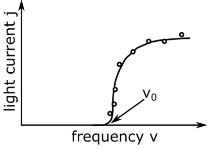
• In contrast, a characteristic dependence of electron emission from the frequency of the incident radiation is detected. Figure 1.2 shows this dependence. Apparently there is a minimum light frequency ν

(still dependent on the material) so that no matter how intense the radiation is, does not generate photo-electrons when the light frequency is lower than ν

. Also, this phenomenon is in contradiction to the classical wave theory of light. This namely means that the photoelectric effect occurs at each frequency, assum- ing that the intensity of the irradiated light strong is enough to beat electrons from the surface.

• In addition, the wave theory predicts that in low light radiation, a noticeable time elapse should be switching between the light and the engine where the electron has absorbed enough energy so that it can leave the metal. Experimentally, no such delay was noted.

li ght curr ent j

frequency ν ν ₀

Figure 1.2: Dependence of the electron emission from the frequency of the incident light

1.2.3 E

’

Declaration

In 1905, a decade before M

’

experiment, Albert Einstein proposed, having regard to the sightings of L

, a simple but revolutionary theory of the photoelectric rule effect as:

Φ is the energy that an electron needs to escape from a given metal. This electron absorbs light radiation energy E and it gains kinetic energy:

E

= E − ^Φ _(1.1)

Obviously, emission occurs only when it is greater than Φ . E

postulated analogously as put forward by M

P

, a quantum hypothesis in another context that the energy of

4

the light radiation from the electron is only in quanta of size:

E = h ν (1.2)

and can be absorbed. Here, ν is the frequency of light and h is P

’

constant. For the kinetic energy of the photo-electrons, it is obtained:

E

= h ν − ^Φ _{. (1.3)}

Not all electrons need as much energy Φ to get out of the metal. However, for each metal, there is a minimum energy Φ

, which is called the work function. Therefore, the maximum kinetic energy of a photo-electron is:

E

= h ν − Φ

. (1.4)

It follows that for frequency ν

=

/

, the maximum kinetic energy E

= 0 becomes; i.e. ν

is that minimum frequency of occurrence of the photoelectric effect. For frequencies ν smaller than ν

, it is h ν smaller than the minimum required work function Φ

and therefore, is no photo-emission on it.

5

1.3 Experiment

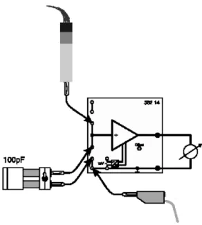
1.3.1 Equipment

Components Number

Optical system with a photocell 1

Electrometer amplifier 1

Measuring capacitor with a button 1

Multimeter 1

Coaxial measuring cable 1

Experimental leads 5

Power supply for high-pressure mercury lamp 1 1.3.2 Experimental Setup

a

c e f

i

j

k

l d

Figure 1.3: Compact arrangement of the optical system.

a) High-pressure mercury lamp, b) Slide,

c) Collecting lens (f=50mm), d) Gap,

e) Imaging lens (f=100mm), f) Vision prism with collar, g) Mirror,

h) Terminals of the test leads,

i) Guiding wire of the pivotable arm of the photocell, j) Collecting lens (f=50mm),

k) Photocell,

l) Window and dimmed slide

6

In the present experimental setup (see Figure 1.3), the light of a mercury high pressure lamp is spectrally dispersed. The individual lines of the spectrum (see Table 1.1) are successively di- rected onto a photo-cathode. The outgoing photo-electron is collected by an annular platinum anode.

The resulting photo current j, slowly charges the capacitor stronger on electrometer. This means that charges from the platinum anode migrate to the capacitor. For the relationship between charge Q and voltage V

across the capacitor with capacitance C gives:

V

= ^Q C

The voltage across the capacitor thus corresponds to the voltage between the anode and cath- ode photocell. This leads to an electric field in the cell, which the photo-current j counteracts.

The charges will flow more on the capacitor, the counter voltage is greater and the current is smaller. Finally, if the electric potential, which has overcome the electrons, becomes larger than their kinetic energy (eV ≥ _E

), then the current disappears (e is the electron charge).

In between, the critical reverse voltage V

and the frequency of the incident light exists so that the following linear relationship is:

E

= V

e = h ν − Φ

(1.5)

⇒ _V

= ^h

e ν − ^Φ

e (1.6)

With the experimentally determined frequency dependence of V

, the light quantity hypothe- ses are tested directly and the constant h is determined.

1.3.3 Implementation

Color and wavelength [nm] and frequency ν [10

Hz]

red 650 4.6

yellow 578 5.19

green 546 5.49

turquoise 493 6.08

blue 436 6.88

purple 405 7.41

Table 1.1: Main lines of the Hg-Lamp

• Put the capacitor switch to the input of the electrometer amplifier.

• Connect the coaxial cable to the optical system (h) as in Figure 1.3) and the inputs (large connector) or the ground (small plug) of the electrometer amplifier.

• Connect the two jack outputs of the optical system with a short experimental lead. Con- nect them now with another experiment lead to the ground of the electrometer amplifier.

• Connect the ground of the electrometer amplifier with another experimental lead to the ground on the power strip.

• Buckle the multimeter to the output of the electrometer amplifier.

7

Figure 1.4: Electrometer Amplifier

• Unlock the high pressure mercury lamp. Note that they can be very hot when in use!

• Adjust the optics so that the plane of the last condenser lens (k) in Figure 1.3) has clearly separated spectral lines visible.

• Swivel the threaded guide of the photocell to the first spectral line. Mark the shadow with a pen, which is visible in the observation window that shows the position of the photocell.

• During the measurement, rest the metal lid and the slide so the observation window can be closed.

1.3.4 Tasks for Evaluation

1. Formulate the photoelectric cell as described above to the first spectral line. Discharge the capacitor by pressing the button. Wait about a minute until the voltage has stabilized.

Now you can read the counter voltage V

off the multimeter. Note that this structure is very sensitive to inductive interference. This means that during the measurement you should not move the experiment leads.

2. Repeat the measurement for each of the remaining lines (at least five) and plot the data in the table.

3. Plot with plot V

and ∆ V

as a function of ν (see Table 1.1), create a linear fit, and deter- mine P

’

constant h. Find h from the slope of line, which is determined by Eq.

1.6. The elementary charge e is expected to be known.

4. . Compare the value with the tabulated value of precision measurement (a theoretical mathematical value does not exist!) and discuss the uncertainties of your fits.

8

1.4 Literature

• Paul A. Tipler, Physik für Naturwissenschaftler und Ingenieure, Spektrum

• Horst Stöcker, Taschenbuch der Physik, Verlag Harri Deutsch

9

10