–Monograph– ALBERTA DesignofAdaptiveFiniteElementSoftware:TheFiniteElementToolbox AlfredSchmidtandKunibertG.Siebert

(1)

Alfred Schmidt and Kunibert G. Siebert

Design of Adaptive Finite Element Software:

The Finite Element Toolbox ALBERTA

SPIN Springer’s internal project number, if known

– Monograph –

October 18, 2004

Springer

Berlin Heidelberg New York Hong Kong London

Milan Paris Tokyo

(2)

(3)

Preface

During the last years, scientific computing has become an important research branch located between applied mathematics and applied sciences and engineering. Nowadays, in numerical mathematics not only simple model problems are treated, but modern and well-founded mathematical algorithms are applied to solve complex problems of real life applications. Such applications are demanding for computational realization and need suitable and robust tools for a flexible and efficient implementation. Modularity and abstract concepts allow for an easy transfer of methods to different applications.

Inspired by and parallel to the investigation of real life applications, numerical mathematics has built and improved many modern algorithms which are now standard tools in scientiﬁc computing. Examples are adaptive methods, higher order discretizations, fast linear and non-linear iterative solvers, multi-level algorithms, etc. These mathematical tools are able to reduce computing times tremendously and for many applications a simulation can only be realized in a reasonable time frame using such highly eﬃcient algorithms.

A very flexible software is needed when working in both fields of scientific computing and numerical mathematics. We developed the toolboxALBERTA¹ for meeting these requirements. Our intention in the design of ALBERTAis threefold: First, it is a toolbox for fast and flexible implementation of efficient software for real life applications, based on the modern algorithms mentioned above. Secondly, in an interplay with mathematical analysis,ALBERTAis an environment for improving existent, or developing new numerical methods.

And ﬁnally, it allows the direct integration of such new or improved methods in existing simulation software.

Before havingALBERTA, we worked with a variety of solvers, each designed for the solution of one single application. Most of them were based on data structures speciﬁcally designed for one single application. A combination of diﬀerent solvers or exchanging modules between programs was hard to do.

1The original name of the toolbox was ALBERT. Due to copyright reasons, we had to rename it and we have chosenALBERTA.

(4)

Facing these problems, we wanted to develop a general adaptive ﬁnite element environment, open for implementing a large class of applications, where an exchange of modules and a coupling of diﬀerent solvers is easy to realize.

Such a toolbox has to be based on a solid concept which is still open for ex- tensions as science develops. Such a solid concept can be derived from a mathematical abstraction of problem classes, numerical methods, and solvers. Our mathematical view of numerical algorithms, especially finite element methods, is based on our education and scientific research in the departments for applied mathematics at the universities of Bonn and Freiburg. This view point has greatly inspired the abstract concepts of ALBERTAas well as their practical realization, reflected in the main data structures. The robustness and flexible extensibility of our concept was approved in various applications from physics and engineering, like computational fluid dynamics, structural mechanics, in- dustrial crystal growth, etc. as well as by the validation of new mathematical methods.

ALBERTAis a library with data structures and functions for adaptive finite element simulations in one, two, and three space dimension, written in the programming language ANSI-C. Shortly after finishing the implementation of the first version of ALBERTAand using it for first scientific applications, we confronted students with it in a course about finite element methods. The idea was to work on more interesting projects in the course and providing a strong foundation for an upcoming diploma thesis. Using ALBERTAin education then required a documentation of data structures and functions. The numerical course tutorials were the basis for a description of the background and concepts of adaptive finite elements.

The combination of the abstract and concrete description resulted in a manual forALBERTAand made it possible that it is now used world wide in universities and research centers. The interest from other scientists motivated a further polishing of the manual as well as the toolbox itself, and resulted in this book.

These notes are organized as follows: In Chapter 1 we describe the concepts of adaptive ﬁnite element methods and its ingredients like the domain discretization, ﬁnite element basis functions and degrees of freedom, numerical integration via quadrature formulas for the assemblage of discrete systems, and adaptive algorithms.

The second chapter is a tutorial for usingALBERTAwithout giving much details about data structures and functions. The implementation of three model problems is presented and explained. We start with the easy and straight forward implementation of the Poisson problem to learn about the basics of ALBERTA. The examples with the implementation of a nonlinear reaction-diﬀusion problem and the time dependent heat equation are more involved and show the tools of ALBERTAfor attacking more complex problems. The chapter is closed with a short introduction to the installation of the

(5)

Preface VII ALBERTAdistribution enclosed to this book in a UNIX/Linux environment.

Visit theALBERTAweb site http://www.alberta-fem.de/

for updates, more information, FAQ, contributions, pictures from diﬀerent projects, etc.

The realization of data structures and functions inALBERTAis based on the abstract concepts presented in Chapter 1. A detailed description of all data structures and functions of ALBERTAis given in Chapter 3. The book closes with separate lists of all data types, symbolic constants, functions, and macros.

The cover picture of this book shows the ALBERTAlogo, combined with a locally reﬁned cogwheel mesh [17], and the norm of the velocity from a calculation of edge tones in a ﬂute [4].

Starting first as a two-men-project,ALBERTAis evolving and now there are more people maintaining and extending it. We are grateful for a lot of substantial contributions coming from: Michael Fried, who was the first brave man besides us to useALBERT, Claus-Justus Heine, Daniel Köster, and Oliver Kriessl. Daniel and Claus in particular set up the GNU configure tools for an easy, platform-independent installation of the software.

We are indebted to the authors of the gltools, especially J¨urgen Fuhrmann, and also to the developers of GRAPE, especially Bernard Haasdonk, Robert Kl¨ofkorn, Mario Ohlberger, and Martin Rumpf.

We want to thank the Department of Mathematics at the University of Maryland (USA), in particular Ricardo H. Nochetto, where part of the documentation was written during a visit of the second author. We appreciate the invitation of the Isaac Newton Institute in Cambridge (UK) where we could meet and work intensively on the revision of the manual for three weeks.

We thank our friends, distributed all over the world, who have pointed out a lot of typos in the manual and suggested several improvements for ALBERTA.

Last but not least, ALBERTA would not have come into being without the stimulating atmosphere in the group in Freiburg, which was the perfect environment for working on this project. We want to express our gratitude to all former colleagues, especially Gerhard Dziuk.

Bremen and Augsburg, October 2004 Alfred Schmidt and Kunibert G. Siebert

(6)

(7)

Introduction

Finite element methods provide a widely used tool for the solution of problems with an underlying variational structure. Modern numerical analysis and im- plementations for finite elements provide more and more tools for the efficient solution of large-scale applications. Efficiency can be increased by using local mesh adaption, by using higher order elements, where applicable, and by fast solvers.

Adaptive procedures for the numerical solution of partial diﬀerential equa- tions started in the late 70’s and are now standard tools in science and engineering. Adaptive ﬁnite element methods are a meaningful approach for handling multi scale phenomena and making realistic computations feasible, specially in 3d.

There exists a vast variety of books about ﬁnite elements. Here, we only want to mention the books by Ciarlet [25], and Brenner and Scott [23] as the most prominent ones. The book by Brenner and Scott also contains an introduction to multi-level methods.

The situation is completely different for books about adaptive finite elements. Only few books can be found with introductory material about the mathematics of adaptive finite element methods, like the books by Verfürth [73], and Ainsworth and Oden [2]. Material about more practical issues like adaptive techniques and refinement procedures can for example be found in [3, 5, 8, 44, 46].

Another basic ingredient for an adaptive ﬁnite element method is the a posteriori error estimator which is main object of interest in the analysis of adaptive methods. While a general theory exists for these estimators in the case of linear and mildly nonlinear problems [10, 73], highly nonlinear problems usually still need a special treatment, see [24, 33, 54, 55, 69] for instance. There exist a lot of diﬀerent approaches to (and a large number of articles about) the derivation of error estimates, by residual techniques, dual techniques, solution of local problems, hierarchical approaches, etc., a fairly incomplete list of references is [1, 3, 7, 13, 21, 36, 52, 72].

(12)

Although adaptive ﬁnite element methods in practice construct a sequence of discrete solutions which converge to the true solution, this convergence could only be proved recently for linear elliptic problem [50, 51, 52] and for the nonlinear Laplacian [70], based on the fundamental paper [31]. For a mod- iﬁcation of the convergent algorithm in [50], quasi-optimality of the adaptive method was proved in [16] and [67].

During the last years there has been a great progress in designing ﬁnite element software. It is not possible to mention all freely available packages.

Examples are [5, 11, 12, 49, 62], and an continuously updated list of other available ﬁnite element codes and resources can for instance be found at

http://www.engr.usask.ca/~macphed/finite/fe_resources/.

Adaptive ﬁnite element methods and basic concepts of ALBERTA Finite element methods calculate approximations to the true solution in some ﬁnite dimensional function space. This space is built fromlocal function spaces, usually polynomials of low order, on elements of a partitioning of the domain (the mesh). An adaptive method adjusts this mesh (or the local function space, or both) to the solution of the problem. This adaptation is based on information extracted froma posteriori error estimators.

The basic iteration of an adaptive ﬁnite element code for a stationary problem is

• assemble and solve the discrete system;

• calculate the error estimate;

• adapt the mesh, when needed.

For time dependent problems, such an iteration is used in each time step, and the step size of a time discretization may be subject to adaptivity, too.

The core part of every ﬁnite element program is the problem dependent assembly and solution of the discretized problem. This holds for programs that solve the discrete problem on a ﬁxed mesh as well as for adaptive methods that automatically adjust the underlying mesh to the actual problem and solution.

In the adaptive iteration, the assemblage and solution of a discrete system is necessary after each mesh change. Additionally, this step is usually the most time consuming part of that iteration.

A general finite element toolbox must provide flexibility in problems and finite element spaces while on the other hand this core part can be performed efficiently. Data structures are needed which allow an easy and efficient implementation of the problem dependent parts and also allow to use adaptive methods, mesh modification algorithms, and fast solvers for linear and nonlinear discrete problems by calling library routines. On one hand, large flexibility is needed in order to choose various kinds of finite element spaces, with higher order elements or combinations of different spaces for mixed methods or systems. On the other hand, the solution of the resulting discrete systems may

(13)

Introduction 3 proﬁt enormously from a simple vector–oriented storage of coeﬃcient vectors and matrices. This also allows the use of optimized solver and BLAS libraries.

Additionally, multilevel preconditioners and solvers may proﬁt from hierarchy information, leading to highly eﬃcient solvers for the linear (sub–) problems.

ALBERTA[59, 60, 62] provides all those tools mentioned above for the ef- ﬁcient implementation and adaptive solution of general nonlinear problems in two and three space dimensions. The design of theALBERTAdata structures allows a dimension independent implementation of problem dependent parts.

The mesh adaptation is done by local reﬁnement and coarsening of mesh elements, while the same local function space is used on all mesh elements.

Starting point for the design of ALBERTAdata structures is the abstract concept of a finite element space defined (similar to the definition of a single finite element by Ciarlet [25]) as a triple consisting of

• a collection ofmesh elements;

• a set of local basis functions on a single element, usually a restriction of global basis functions to a single element;

• a connection of local and global basis functions giving global degrees of freedom for a ﬁnite element function.

This directly leads to the deﬁnition of three main groups of data structures:

• data structures for geometric information storing the underlying mesh together with element coordinates, boundary type and geometry, etc.;

• data structures for ﬁnite element information providing values of local basis functions and their derivatives;

• data structures for algebraic information linking geometric data and ﬁnite element data.

Using these data structures, the finite element toolboxALBERTAprovides the whole abstract framework like finite element spaces and adaptive strategies, together with hierarchical meshes, routines for mesh adaptation, and the com- plete administration of finite element spaces and the corresponding degrees of freedom (DOFs) during mesh modifications. The underlying data structures allow a flexible handling of such information. Furthermore, tools for numerical quadrature, matrix and load vector assembly as well as solvers for (linear) problems, like conjugate gradient methods, are available.

A speciﬁc problem can be implemented and solved by providing just some problem dependent routines for evaluation of the (linearized) diﬀerential op- erator, data, nonlinear solver, and (local) error estimators, using all the tools above mentioned from a library.

Both geometric and finite element information strongly depend on the space dimension. Thus, mesh modification algorithms and basis functions are implemented for one (1d), two (2d), and three (3d) dimensions separately and are provided by the toolbox. Everything besides that can be formulated in such a way that the dimension only enters as a parameter (like size of local coordinate vectors, e.g.). For usual finite element applications this results in

(14)

a dimension independent programming, where all dimension dependent parts are hidden in a library. This allows a dimension independent programming of applications to the greatest possible extent.

The remaining parts of the introduction give a short overview over the main concepts, details are then given in Chapter 1.

The hierarchical mesh

The underlying mesh is a conforming triangulation of the computational domain into simplices, i.e. intervals (1d), triangles (2d), or tetrahedra (3d). The simplicial mesh is generated by refinement of a given initial triangulation. Re- fined parts of the mesh can be de–refined, but elements of the initial triangulation (macro elements) must not be coarsened. The refinement and coarsening routines construct a sequence of nested meshes with a hierarchical structure.

InALBERTA, the recursive reﬁnement by bisection is implemented, using the notation of Kossaczk´y [44].

During refinement, new degrees of freedom are created. A single degree of freedom is shared by all elements which belong to the support of the corresponding finite element basis function (compare next paragraph). The mesh refinement routines must create a new DOF only once and give access to this DOF from all elements sharing it. Similarly, DOFs are handled during coarsening. This is done in cooperation with the DOF administration tool, see below.

The bisectioning refinement of elements leads naturally to nested meshes with the hierarchical structure of binary trees, one tree for every element of the initial triangulation. Every interior node of that tree has two pointers to the two children; the leaf elements are part of the actual triangulation, which is used to define the finite element space(s). The whole triangulation is a list of given macro elements together with the associated binary trees. The hierarchical structure allows the generation of most information by the hierarchy, which reduces the amount of data to be stored. Some information is stored on the (leaf) elements explicitly, other information is located at the macro elements and is transfered to the leaf elements while traversing through the binary tree. Element information about vertex coordinates, domain bound- aries, and element adjacency can be computed easily and very fast from the hierarchy, when needed. Data stored explicitly at tree elements can be reduced to pointers to the two possible children and information about local DOFs (for leaf elements). Furthermore, the hierarchical mesh structure directly leads to multilevel information which can be used by multilevel preconditioners and solvers.

Access to mesh elements is available solely via routines which traverse the hierarchical trees; no direct access is possible. The traversal routines can give access to all tree elements, only to leaf elements, or to all elements which belong to a single hierarchy level (for a multilevel application, e.g.). In order to perform operations on visited elements, the traversal routines call a subroutine

(15)

Introduction 5 which is given to them as a parameter. Only such element information which is needed by the current operation is generated during the tree traversal.

Finite elements

The values of a finite element function or the values of its derivatives are uniquely defined by the values of its DOFs and the values of the basis functions or the derivatives of the basis functions connected with these DOFs. We follow the concept of finite elements which are given on a single element S in local coordinates: Finite element functions on an elementS are defined by a finite dimensional function space ¯Pon a reference element ¯S and the (one to one) mapping λ^S : ¯S →S from the reference element ¯S to the element S. In this situation the non vanishing basis functions on an arbitrary element are given by the set of basis functions of ¯Pin local coordinatesλ^S. Also, derivatives are given by the derivatives of basis functions on ¯Pand derivatives ofλ^S.

Each local basis function on S is uniquely connected to a global degree of freedom, which can be accessed from S via the DOF administration tool.

ALBERTAsupports basis functions connected with DOFs, which are located at vertices of elements, at edges, at faces (in 3d), or in the interior of elements.

DOFs at a vertex are shared by all elements which meet at this vertex, DOFs at an edge or face are shared by all elements which contain this edge or face, and DOFs inside an element are not shared with any other element.

The support of the basis function connected with a DOF is the patch of all elements sharing this DOF.

For a very general approach, we only need a vector of the basis functions (and its derivatives) on ¯S and a function for the communication with the DOF administration tool in order to access the degrees of freedom connected to local basis functions. By such information every ﬁnite element function (and its derivatives) is uniquely described on every element of the mesh.

During mesh modifications, finite element functions must be transformed to the new finite element space. For example, a discrete solution on the old mesh yields a good initial guess for an iterative solver and a smaller number of iterations for a solution of the discrete problem on the new mesh. Usu- ally, these transformations can be realized by a sequence of local operations.

Local interpolations and restrictions during refinement and coarsening of elements depend on the function space ¯Pand the refinement of ¯S only. Thus, the subroutine for interpolation during an atomic mesh refinement is the efficient implementation of the representation of coarse grid functions by fine grid functions on ¯Sand its refinement. A restriction during coarsening is implemented using similar information.

Lagrange ﬁnite element spaces up to order four are currently implemented in one, two, and three dimensions. This includes the communication with the DOF administration as well as the interpolation and restriction routines.

(16)

Degrees of freedom

Degrees of freedom (DOFs) connect finite element data with geometric information of a triangulation. For general applications, it is necessary to handle several different sets of degrees of freedom on the same triangulation. For example, in mixed finite element methods for the Navier-Stokes problem, different polynomial degrees are used for discrete velocity and pressure functions.

During adaptive reﬁnement and coarsening of a triangulation, not only elements of the mesh are created and deleted, but also degrees of freedom together with them. The geometry is handled dynamically in a hierarchical binary tree structure, using pointers from parent elements to their children.

For data corresponding to DOFs, which are usually involved with matrix–

vector operations, simpler storage and access methods are more eﬃcient. For that reason every DOF is realized just as an integer index, which can easily be used to access data from a vector or to build matrices that operate on vectors of DOF data. This results in a very eﬃcient access during matrix/vector operations and in the possibility to use libraries for the solution of linear systems with a sparse system matrix ([29], e.g.).

Using this realization of DOFs two major problems arise:

• During reﬁnement of the mesh, new DOFs are added, and additional indices are needed. The total range of used indices has to be enlarged. At the same time, all vectors and matrices that use these DOF indices have to be adjusted in size, too.

• During coarsening of the mesh, DOFs are deleted. In general, the deleted DOF is not the one which corresponds to the largest integer index. Holes with unused indices appear in the total range of used indices and one has to keep track of all used and unused indices.

These problems are solved by a general DOF administration tool. During reﬁnement, it enlarges the ranges of indices, if no unused indices produced by a previous coarsening are available. During coarsening, a book–keeping about used and unused indices is done. In order to reestablish a contiguous range of used indices, a compression of DOFs can be performed; all DOFs are renumbered such that all unused indices are shifted to the end of the index range, thus removing holes of unused indices. Additionally, all vectors and matrices connected to these DOFs are adjusted correspondingly. After this process, vectors do not contain holes anymore and standard operations like BLAS1 routines can be applied and yield optimal performance.

In many cases, information stored in DOF vectors has to be adjusted to the new distribution of DOFs during mesh reﬁnement and coarsening.

Each DOF vector can provide pointers to subroutines that implements these operations on data (which usually strongly depend on the corresponding ﬁnite element basis). Providing such a pointer, a DOF vector will automatically be transformed during mesh modiﬁcations.

(17)

Introduction 7 All tasks of the DOF administration are performed automatically during refinement and coarsening for every kind and combination of finite elements defined on the mesh.

Adaptive solution of the discrete problem

The aim of adaptive methods is the generation of a mesh which is adapted to the problem such that a given criterion, like a tolerance for the estimated error between exact and discrete solution, is fulfilled by the finite element solution on this mesh. An optimal mesh should be as coarse as possible while meeting the criterion, in order to save computing time and memory requirements. For time dependent problems, such an adaptive method may include mesh changes in each time step and control of time step sizes. The philosophy implemented in ALBERTAis to change meshes successively by local refinement or coarsening, based on error estimators or error indicators, which are computed a posteriori from the discrete solution and given data on the current mesh.

Several adaptive strategies are proposed in the literature, that give criteria which mesh elements should be marked for reﬁnement. All strategies are based on the idea of an equidistribution of the local error to all mesh elements.

Babuˇska and Rheinboldt [3] motivate that for stationary problems a mesh is almost optimal when the local errors are approximately equal for all elements.

So, elements where the error indicator is large will be marked for reﬁnement, while elements with a small estimated indicator are left unchanged or are marked for coarsening. In time dependent problems, the mesh is adapted to the solution in every time step using a posteriori information like in the stationary case. As a ﬁrst mesh for the new time step we use the adaptive mesh from the previous time step. Usually, only few iterations of the adaptive procedure are then needed for the adaptation of the mesh for the new time step. This may be accompanied by an adaptive control of time step sizes.

Given pointers to the problem dependent routines for assembling and solution of the discrete problems, as well as an error estimator/indicator, the adaptive method for finding a solution on a quasi–optimal mesh can be performed as a black–box algorithm. The problem dependent routines are used for the calculation of discrete solutions on the current mesh and (local) error estimates. Here, the problem dependent routines heavily make use of library tools for assembling system matrices and right hand sides for an arbitrary finite element space, as well as tools for the solution of linear or nonlinear discrete problems. On the other hand, any specialized algorithm may be added if needed. The marking of mesh elements is based on general refinement and coarsening strategies relying on the local error indicators. During the following mesh modification step, DOF vectors are transformed automatically to the new finite element spaces as described in the previous paragraphs.

(18)

Dimension independent program development

Using black–box algorithms, the abstract deﬁnition of basis functions, quadrature formulas and the DOF administration tool, only few parts of the ﬁnite element code depend on the dimension. Usually, all dimension dependent parts are hidden in the library. Hence, program development can be done in 1d or 2d, where execution is usually much faster and debugging is much easier (because of simple 1d and 2d visualization, e.g., which is much more involved in 3d). With no (or maybe few) additional changes, the program will then also work in 3d. This approach leads to a tremendous reduction of program development time for 3d problems.

Notations. For a diﬀerentiable function f: Ω →R on a domain Ω⊂R^d, d= 1,2,3, we set

∇f(x) = (f_,x₁(x), . . . , f_,x_d(x)) = ∂

∂x₁f(x), . . . , ∂

∂x_df(x)

and

D²f(x) = (f_,x_k_x_l)_k,l=1,...d= ∂²

∂x_kx_lf(x)

k,l=1,...d

.

For a vector valued, diﬀerentiable function f = (f₁, . . . , f_n) : Ω → Rⁿ we write

∇f(x) = (f_i,x₁(x), . . . , f_i,x_d(x))_i=1,...,n = ∂

∂x₁f_i(x), . . . , ∂

∂x_df_i(x)

i=1,...,n

and

D²f(x) = (f_i,x_k_x_l)i=1,...,n k,l=1,...d =

∂²

∂x_kx_lf_i(x)

i=1,...,n k,l=1,...d

. ByL^p(Ω), 1≤p≤ ∞, we denote the usual Lebesgue spaces with norms

f_L^p_(Ω)=

Ω

|f(x)|^pdx _1/p

forp <∞ and

f_L^∞_(Ω)= ess sup

x∈Ω |f(x)|.

The Sobolev space of functionsu∈L²(Ω) with weak derivatives∇u∈L²(Ω) is denoted byH¹(Ω) with semi norm

|u|_H¹_(Ω)=

Ω

|∇u(x)|²dx _1/2

and norm

u_H¹_(Ω)=

u²_L2(Ω)+|u|²_H1(Ω)

_1/2 .

(19)

1 Concepts and abstract algorithms

1.1 Mesh reﬁnement and coarsening

In this section, we describe the basic algorithms for the local reﬁnement and coarsening of simplicial meshes in two and three dimensions. In 1d the grid is built from intervals, in 2d from triangles, and in 3d from tetrahedra. We restrict ourselves here to simplicial meshes, for several reasons:

1. A simplex is one of the most simple geometric types and complex domains may be approximated by a set of simplices quite easily.

2. Simplicial meshes allow local reﬁnement (see Fig. 1.1) without the need of non–conforming meshes (hanging nodes), parametric elements, or mixture of element types (which is the case for quadrilateral meshes, e.g., see Fig.

1.2).

3. Polynomials of any degree are easily represented on a simplex using local (barycentric) coordinates.

Fig. 1.1.Global and local reﬁnement of a triangular mesh.

First of all we start with the deﬁnition of a simplex, parametric simplex and triangulation:

Deﬁnition 1.1 (Simplex).

a) Let a₀, . . . , a_d ∈Rⁿ be given such that a₁−a₀, . . . , a_d−a₀ are linear in- dependent vectors inRⁿ. The convex set

(20)

Fig. 1.2. Local refinements of a rectangular mesh: with hanging nodes, conforming closure using bisected rectangles, and conforming closure using triangles. Using a conforming closure with rectangles, a local refinement has always global effects up to the boundary.

S= conv hull{a₀, . . . , a_d} is called a d–simplexinRⁿ. For k < dlet

S= conv hull{a₀, . . . , a_k} ⊂∂S

be ak–simplex with a₀, . . . , a_k ∈ {a₀, . . . , a_d}. ThenS is called a k–sub–

simplexofS. A0–sub–simplex is called vertex, a1–sub–simplex edgeand a2–sub–simplex face.

b) The standard simplex inR^d is deﬁned by

Sˆ= conv hull{aˆ₀= 0,ˆa₁=e₁, . . . ,aˆ_d=e_d}, wheree_i are the unit vectors inR^d.

c) Let F_S: ˆS → S ⊂ Rⁿ be an invertible, differentiable mapping. Then S is called a parametricd–simplex inRⁿ. The k–sub–simplices S of S are given by the images of the k–sub–simplices Sˆ of S. Thus, the verticesˆ a₀, . . . , a_d ofS are the points F_S(â₀), . . . , F_S(â_d).

d) For a d–simplexS, we deﬁne

h_S := diam(S) and ρ_S := sup{2r;B_r⊂S is ad–ball of radius r}, the diameter and inball–diameter ofS.

Remark 1.2.Everyd–simplexS inRⁿ is a parametric simplex. Deﬁning the matrixA_S ∈R^n×d by

A_S =

⎡

⎢⎢

⎣

... ... a₁−a₀· · · a_d−a₀

... ...

⎤

⎥⎥

⎦,

the parameterizationF_S: ˆS →S is given by

F_S(ˆx) =A_Sxˆ+a₀. (1.1) SinceF_S is affine linear it is differentiable. It is easy to check thatF_S: ˆS→S is invertible and thatF_S(â_i) =a_i,i= 0, . . . , dholds.

(21)

1.1 Mesh reﬁnement and coarsening 11

Deﬁnition 1.3 (Triangulation).

a) LetS be a set of (parametric)d–simplices and deﬁne Ω= interior

S∈S

S⊂Rⁿ.

We callSa conforming triangulationofΩ, iff for two simplicesS₁, S₂∈ S withS₁=S₂ the intersectionS₁∩S₂is either empty or a completek–sub–

simplex of bothS₁ andS₂ for some0≤k < d.

b) Let Sk,k≥0, be a sequence of conforming triangulations. This sequence is called (shape) regular, iff

sup

k∈N0

max

S∈Sk

max

x∈ˆ Sˆ

cond(DF_S^t(ˆx)·DF_S(ˆx))<∞ (1.2) holds, whereDF_S is the Jacobian ofF_S andcond(A) =AA⁻¹denotes the condition number.

Remark 1.4.For a sequenceSk,k≥0, of non–parametric triangulations the regularity condition (1.2) is equivalent to the condition

sup

k∈N0

max

S∈Sk

h_S ρ_S <∞.

In order to construct a sequence of triangulations, we consider the following situation: An initial (coarse) triangulationS0of the domain is given. We call it macro triangulation. It may be generated by hand or by some mesh generation algorithm ([63, 65]).

Some (or all) of the simplices are marked for reﬁnement, depending on some error estimator or indicator. The marked simplices are then reﬁned, i.e.

they are cut into smaller ones. After several refinements, some other simplices may be marked for coarsening. Coarsening tries to unite several simplices marked for coarsening into a bigger simplex. A successive refinement and coarsening will produce a sequence of triangulations S0,S1, . . .. The refinement of single simplices that we describe in the next section produces for every simplex of the macro triangulation only a finite and small number of similarity classes for the resulting elements. The coarsening is more or less the inverse process of refinement. This leads to a finite number of similarity classes for all simplices in the whole sequence of triangulations.

The refinement of non–parametric and parametric simplices is the same topological operation and can be performed in the same way. The actual children’s shape of parametric elements additionally involves the children’s pa- rameterization. In the following we describe the refinement and coarsening for triangulations consisting of non–parametric elements. The refinement of parametric triangulations can be done in the same way, additionally using given parameterizations. Regularity for the constructed sequence can be obtained

(22)

with special properties of the parameterizations for parametric elements and the ﬁnite number of similarity classes for simplices.

Marking criteria and marking strategies for reﬁnement and coarsening are subject of Section 1.5.

1.1.1 Reﬁnement algorithms for simplicial meshes

For simplicial elements, several refinement algorithms are widely used. The discussion about and description of these algorithms mainly centers around refinement in 2d and 3d since refinement in 1d is straight forward.

One example is regular refinement (“red refinement”), which divides every triangle into four similar triangles, see Fig. 1.3. The corresponding refinement algorithm in three dimensions cuts every tetrahedron into eight tetrahedra, and only a small number of similarity classes occur during successive refinements, see [14, 15]. Unfortunately, hanging nodes arise during local regular refinement. To remove them and create a conforming mesh, in two dimensions some triangles have to be bisected (“green closure”). In three dimensions, several types of irregular refinement are needed for the green closure. This creates more similarity classes, even in two dimensions. Additionally, these bisected elements have to be removed before a further refinement of the mesh, in order to keep the triangulations shape regular.

Fig. 1.3. Global and local regular reﬁnement of triangles and conforming closure by bisection.

Another possibility is to use bisection of simplices only. For every element (triangle or tetrahedron) one of its edges is marked as thereﬁnement edge, and the element is reﬁned into two elements by cutting this edge at its midpoint.

There are several possibilities to choose such a refinement edge for a simplex, one example is to use the longest edge; Mitchell [48] compared different approaches. We focus on an algorithm where the choice of refinement edges on the macro triangulation prescribes the refinement edges for all simplices that are created during mesh refinement. This makes sure that shape regularity of the triangulations is conserved.

In two dimensions we use thenewest vertex bisection (in Mitchell’s notation) and in three dimensions the bisection procedure of Kossaczk´y described in [44]. We use the convention, that all vertices of an element are given ﬁxed local indices. Valid indices are 0, 1, for vertices of an interval, 0, 1, and 2 for

(23)

1.1 Mesh refinement and coarsening 13 vertices of a triangle, and 0, 1, 2, and 3 for vertices of a tetrahedron. Now, the refinement edge for an element is fixed to be the edge between the vertices with local indices 0 and 1. Here we use the convention that in 1d the element itself is called “refinement edge”.

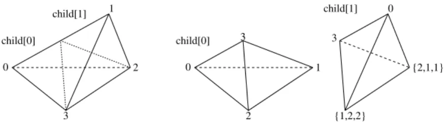
During refinement, the new vertex numbers, and thereby the refinement edges, for the newly created child simplices are prescribed by the refinement algorithm. For both children elements, the index of the newly generated vertex at the midpoint of this edge has the highest local index (2 resp. 3 for triangles and tetrahedra). These numbers are shown in Fig. 1.4 for 1d and 2d, and in Fig. 1.5 for 3d. In 1d and 2d this numbering is the same for all refinement levels. In 3d, one has to make some special arrangements: the numbering of the second child’s vertices does depend on the type of the element. There exist three different element types 0, 1, and 2. The type of the elements on the macro triangulation can be prescribed (usually type 0 tetrahedron). The type of the refined tetrahedra is recursively given by the definition that the type of a child element is ((parent’s type + 1) modulo 3). In Fig. 1.5 we used the following convention: for the index set{1,2,2}onchild[1]of a tetrahedron of type0we use the index1and for a tetrahedron of type 1and2the index 2. Fig. 1.6 shows successive refinements of a type 0 tetrahedron, producing tetrahedra of types 1, 2, and 0 again.

child[0] child[1]

0 1

1 0

0 1 0 1

2

child[0] child[1]

0

1

2 2 0

child[0] child[1]

Fig. 1.4.Numbering of nodes on parent and children for intervals and triangles.

1

0 2

3 child[0]

child[1]

0 1 child[0]

0

{2,1,1}

3 3

2 {1,2,2}

child[1]

Fig. 1.5.Numbering of nodes on parent and children for tetrahedra.

By the above algorithm the reﬁnements of simplices are totally determined by the local vertex numbering on the macro triangulation, plus a prescribed type for every macro element in three dimensions. Furthermore, a successive reﬁnement of every macro element only produces a small number of similarity

(24)

2 0 3

1 child[1]

0 2

3 1

child[0] 2 0

1 3 child[1]

0

2 1 3 child[0]

1 child[0]

1

0 2

3

Type 0:

Type 1:

Type 2:

Type 0:

0 2

3 1

child[0]

0 2

3 1

child[1]

0

2

3 child[1]

0

3

2

1

0 3

child[0] 2

1 3 0 2 child[1]

1 0

3 2 child[0]

1

0 3

2 child[1]

1

0 3 2

child[1]

1

0 3 2

child[0]

Fig. 1.6.Successive reﬁnements of a type 0 tetrahedron.

classes. In case of the “generic” triangulation of a (unit) square in 2d and cube in 3d into two triangles resp. six tetrahedra (see Fig. 1.7 for a single triangle and tetrahedron from such a triangulation – all other elements are generated by rotation and reflection), the numbering and the definition of the refinement edge during refinement of the elements guarantee that always the longest edge will be the refinement edge and will be bisected, see Fig. 1.8.

The refinement of a given triangulation now uses the bisection of single elements and can be performed eitheriteratively orrecursively. In 1d, bisection only involves the element which is subject to refinement and thus is a completely local operation. Both variants of refining a given triangulation are the same. In 2d and 3d, bisection of a single element usually involves other elements, resulting in two different algorithms.

For tetrahedra, the first description of such a refinement procedure was given by Bänsch using the iterative variant [8]. It abandons the requirement of one to one inter–element adjacencies during the refinement process and thus needs the intermediate handling of hanging nodes. Two recursive algorithms, which do not create such hanging nodes and are therefore easier to implement, are published by Kossaczký [44] and Maubach [46]. For a special class of

(25)

1.1 Mesh reﬁnement and coarsening 15 macro triangulations, they result in exactly the same tetrahedral meshes as the iterative algorithm.

In order to keep the mesh conforming during refinement, the bisection of an edge is allowed only when such an edge is the refinement edge for all elements which share this edge. Bisection of an edge and thus of all elements around the edge is theatomic refinement operation, and no other refinement operation is allowed. See Figs. 1.9 and 1.10 for the two and three–dimensional situations.

(0,0,0) (1,0,0)

(1,1,0) (1,1,1)

(1,0) (0,0)

(0,1)

0 1

2 0

1

2 3

Fig. 1.7.Generic elements in two and three dimensions.

(1,0) (0,0)

(0,1)

(0,0,0) (1,0,0)

(1,1,0) (1,1,1)

Fig. 1.8.Reﬁned generic elements in two and three dimensions.

Fig. 1.9.Atomic reﬁnement operation in two dimensions. The common edge is the reﬁnement edge for both triangles.

If an element has to be refined, we have to collect all elements at its refinement edge. In two dimensions this is either the neighbour opposite this edge or there is no other element in the case that the refinement edge belongs

(26)

Fig. 1.10. Atomic reﬁnement operation in three dimensions. The common edge is the reﬁnement edge for all tetrahedra sharing this edge.

to the boundary. In three dimensions we have to loop around the edge and collect all neighbours at this edge. If for all collected neighbours the common edge is the refinement edge too, we can refine the whole patch at the same time by inserting one new vertex in the midpoint of the common refinement edge and bisecting every element of the patch. The resulting triangulation then is a conforming one.

But sometimes the reﬁnement edge of a neighbour is not the common edge.

Such a neighbour isnot compatibly divisible and we have to perform first the atomic refinement operation at the neighbour’s refinement edge. In 2d the child of such a neighbour at the common edge is then compatibly divisible; in 3d such a neighbour has to be bisected at most three times and the resulting tetrahedron at the common edge is then compatibly divisible. The recursive refinement algorithm now reads

Algorithm 1.5 (Recursive reﬁnement of one simplex).

subroutine recursive refine(S, S) do

A:={S∈ S;S is not compatibly divisible with S} for all S ∈ A do

recursive refine(S, S);

end for

A:={S∈ S;S is not compatibly divisible with S} until A=∅

A:={S∈ S;S is element at the refinement edge of S} for all S∈ A

bisect S into S₀ and S₁ S :=S\{S} ∪ {S₀, S₁} end for

In Fig. 1.11 we show a two–dimensional situation where recursion is needed. For all triangles, the longest edge is the refinement edge. Let us as- sume that triangles A and B are marked for refinement. Triangle A can be refined at once, as its refinement edge is a boundary edge. For refinement of triangle B, we have to recursively refine triangles C and D. Again, triangle

(27)

1.1 Mesh refinement and coarsening 17 D can be directly refined, so recursion terminates there. This is shown in the second part of the figure. Back in triangle C, this can now be refined together with its neighbour. After this, also triangle B can be refined together with its neighbour.

C D

A B

Fig. 1.11.Recursive reﬁnement in two dimensions. Triangles A and B are initially marked for reﬁnement.

The reﬁnement of a given triangulationS where some or all elements are marked for reﬁnement is then performed by

Algorithm 1.6 (Recursive reﬁnement algorithm).

subroutine refine(S) for all S∈ S do

if S is marked for refinement recursive refine(S, S) end if

end for

Since we use recursion, we have to guarantee that recursions terminates.

Kossaczk´y [44] and Mitchell [48] proved

Theorem 1.7 (Termination and Shape Regularity). The recursive re- ﬁnement algorithm using bisection of single elements fulﬁlls

1. The recursion terminates if the macro triangulation satisﬁes certain cri- teria.

2. We obtain shape regularity for all elements at all levels.

Remark 1.8.

1. A first observation is, that simplices initially not marked for refinement are bisected, enforced by the refinement of a marked simplex. This is a necessity to obtain a conforming triangulation, also for the regular refinement.

2. It is possible to mark an element for more than one bisection. The natural choice is to mark ad–simplexS fordbisections. Afterdrefinement steps all original edges of S are bisected. A simplex S is refined k times by refining the childrenS₁andS₂k−1 times right after the refinement ofS.

(28)

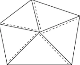
3. The recursion does not terminate for an arbitrary choice of refinement edges on the macro triangulation. In two dimensions, such a situation is shown in Fig. 1.12. The selected refinement edges of the triangles are shown by dashed lines. One can easily see, that there are no patches for the atomic refinement operation. This triangulation can only be refined if other choices of refinement edges are made, or by a non–recursive algorithm.

Fig. 1.12.A macro triangulation where recursion does not stop.

4. In two dimensions, for every macro triangulation it is possible to choose the reﬁnement edges in such a way that the recursion terminates (selecting the ‘longest edge’). In three dimensions the situation is more complicated.

But there is a maybe reﬁned grid such that reﬁnement edges can be chosen in such a way that recursion terminates [44].

1.1.2 Coarsening algorithm for simplicial meshes

The coarsening algorithm is more or less the inverse of the refinement algorithm. The basic idea is to collect all those elements that were created during the refinement at same time, i.e. the parents of these elements build a com- patible refinement patch. The elements must only be coarsened ifall involved elements are marked for coarsening and are of finest level locally, i.e. no element is refined further. The actual coarsening again can be performed in an atomic coarsening operation without the handling of hanging nodes. Infor- mation is passed from all elements onto the parents and the whole patch is coarsened at the same time by removing the vertex in the parent’s common refinement edge (see Figs. 1.13 and 1.14 for the atomic coarsening operation in 2d and 3d). This coarsening operation is completely local in 1d.

During refinement, the bisection of an element can enforce the refinement of an unmarked element in order to keep the mesh conforming. During coarsening, an element must only be coarsened if all elements involved in this operation are marked for coarsening. This is the main difference between refinement and coarsening. In an adaptive method this guarantees that elements with a large local error indicator marked for refinement are refined and no element is coarsened where the local error indicator is not small enough (compare Section 1.5.3).

(29)

1.1 Mesh reﬁnement and coarsening 19

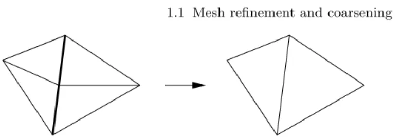
Fig. 1.13.Atomic coarsening operation in two dimensions.

Fig. 1.14.Atomic coarsening operation in three dimensions.

Since the coarsening process is the inverse of the refinement, refinement edges on parent elements are again at their original position. Thus, further refinement is possible with a terminating recursion and shape regularity for all resulting elements.

Algorithm 1.9 (Local coarsening).

subroutine coarsen element(S, S)

A:={S∈ S;S must not be coarsened with S} if A=∅

for all child pairs S₀, S₁ at common coarsening edge do coarse S₀ and S₁ into the parent S

S:=S\{S₀, S₁} ∪ {S} end for

end if

The following routine coarsens as many elements as possible of a given trian- gulationS:

Algorithm 1.10 (Coarsening algorithm).

subroutine coarsen(S) for all S∈ S do

if S is marked for coarsening coarsen element(S, S) end if

end for

Remark 1.11.Also in the coarsening procedure an element can be marked for several coarsening steps. Usually, the coarsening markers for all patch

(30)

elements are cleared if a patch must not be coarsened. If the patch must not be coarsened because one patch element is not of locally ﬁnest level but may coarsened more than once, elements stay marked for coarsening. A coarsening of the ﬁner elements can result in a patch which may then be coarsened.

1.1.3 Operations during reﬁnement and coarsening

The reﬁnement and coarsening of elements can be split into four major steps, which are now described in detail.

Topological reﬁnement and coarsening

The actual bisection of an element is performed as follows: the simplex is cut into two children by inserting a new vertex at the refinement edge. All objects like this new vertex, or a new edge (in 2d and 3d), or face (in 3d) have only to be created once on the refinement patch. For example, all elements share the new vertex and two children triangles share a common edge. The refinement edge is divided into two smaller ones which have to be adjusted to the respective children. In 3d all faces inside the patch are bisected into two smaller ones and this creates an additional edge for each face. All these objects can be shared by several elements and have to be assigned to them.

If neighbour information is stored, one has to update such information for elements inside the patch as well as for neighbours at the patch’s boundary.

In the coarsening process the vertex which is shared by all elements is removed, edges and faces are rejoined and assigned to the respective parent simplices. Neighbour information has to be reinstalled inside the patch and with patch neighbours.

Administration of degrees of freedoms

Single DOFs can be assigned to a vertex, edge, or face and such a DOF is shared by all simplices meeting at the vertex, edge, or face respectively.

Finally, there may be DOFs on the element itself, which are not shared with any other simplex. At each object there may be a single DOF or several DOFs, even for several ﬁnite element spaces.

During reﬁnement new DOFs are created. For each newly created object (vertex, edge, face, center) we have to create the exact amount of DOFs, if DOFs are assigned to the object. For example we have to create vertex DOFs at the midpoint of the reﬁnement edge, if DOFs are assigned to a vertex. Again, DOFs must only be created once for each object and have to be assigned to all simplices having this object in common.

Additionally, all vectors and matrices using these DOFs have automatically to be adjusted in size.