arXiv:1301.5183v3 [hep-ph] 6 Mar 2013
Wolfgang Ochs
Max-Planck-Institut f¨ur Physik, Werner-Heisenberg-Institut, F¨ohringer Ring 6, D-80805 M¨unchen, Germany
E-mail: ochs@mpp.mpg.de
Abstract. Calculations within QCD (lattice and sum rules) find the lightest glueball to be a scalar and with mass in the range of about 1000-1700 MeV. Several phenomenological investigations are discussed which aim at the identification of the scalar meson nonets of lowest mass and the super-numerous states if any. Results on the flavour structure of the light scalarsf0(500), f0(980) andf0(1500) are presented;
the evidence for f0(1370) is scrutinized. A significant surplus of leading clusters of neutral charge in gluon jets is found at LEP in comparison with MCs, possibly a direct signal for glueball production; further studies with more energetic jets at LHC are suggested. As a powerful tool in the identification of the scalar nonets or other multiplets, along with signals from glueballs we propose the exploration of symmetry relations for decay rates ofC= +1 heavy quark states likeχc orχb. Results from χc
decays are discussed; they are not in support of a tetra-quark substructure off0(980).
A minimal scenario for scalar quarkonium-glueball spectroscopy is presented.
1 Introduction 2
2 QCD expectations for glueballs 4
2.1 Quantum numbers . . . . 4
2.2 Lattice QCD. . . . 5
2.3 QCD sum rules . . . . 8
2.4 Conclusions from theory . . . 10
3 Experimental search strategies for glueballs 10 3.1 Quark-gluon constituent structure of hadrons from their decays . . . 10
3.2 Enhanced and suppressed glueball production . . . 15
3.3 Supernumerous states among q q ¯ nonets? . . . 16
4 Spectroscopy of scalar mesons: q¯ q nonets mixing with glueballs 17 4.1 Route 1: (q q) nonet - glueball mixing around 1500 MeV . . . 17 ¯
4.2 Route 2: light glueball around 1 GeV . . . 18
4.3 Route 3: two supernumerous states, broad glueball f
0(1200 − 1600) . . . 20
5 Properties of f
0(500)/σ - comparison with K
0∗(800)/κ 21
5.1 Results on f
0(500)/σ . . . 21
5.2 Comparing elastic ππ and Kπ scattering - a problem with the κ resonance 25 6 Intrinsic structure of f
0(980) 27 6.1 Mixing angle from various observables . . . 27
6.2 Final result on mixing angle . . . 30
6.3 Possible gluonic contribution . . . 30
7 Experimental evidence for f
0(1370) and f
0(1500) - a reassessment 31 7.1 Production in p¯ p annihilation . . . 31
7.2 Search in phase shift analysis of ππ scattering . . . 34
7.3 Decays of D and B into f
0mesons . . . 42
7.4 Decay of J/ψ → φ(1020)f
0, f
0→ ππ, K K ¯ . . . 50
7.5 Central production in hadron hadron collisions . . . 50
7.6 Flavour structure of f
0(1500) from its decays . . . 54
7.7 Production in γγ scattering . . . 56
8 Gluon rich processes in comparison 57 8.1 The Pomeron as an example for mixed gluon and quark components . . 58
8.2 Processes with identified gluons . . . 59
9 Leading systems in gluon jets 59 9.1 Rate of neutral clusters at LEP above Monte Carlo expectations . . . 60
9.2 Proposal for further measurements at the LHC . . . 62
10 [q q] ¯ multiplets and glueballs from symmetry relations: first results from χ
cdecays 65 10.1 Scalar multiplet according to route 2 . . . 65
10.2 Scalar multiplet according to route 1 - tetraquark expectations . . . 67
11 Summary and conclusions 67 11.1 Is there any experimental evidence for the existence of glueballs? . . . 67
11.2 Are there supernumerous states in the scalar sector? . . . 68
11.3 Are there hints towards a gluonic component in isoscalar mesons? . . . . 68
11.4 Future studies of symmetry relations in χ
cdecays . . . 68
11.5 A minimal scenario for scalar quarkonium-glueball spectroscopy . . . 69
List of reprinted figures 79
1. Introduction
The existence of “glueballs”, bound states of gluons, is a consequence of the
self-interaction of gluons within Quantumchromodynamics. Such states have been
considered to appear in analogy to q¯ q states in a quark-gluon theory of hadrons already in 1972 during the early development of QCD [1]. First specific scenarios for glueball spectroscopy on the basis of a quark-gluon field theory with hadrons as colour singlets have been developed by Fritzsch and Minkowski [2] assuming an analogy between massless gluons and photons. Much effort has been devoted during the last 40 years into the theoretical analysis as well as the experimental searches of this new type of hadrons.
While a consensus is reached about the existence and some properties of glueballs in a world without quarks, the details in the full theory are still controversial. Lattice QCD is a formulation of the quark-gluon gauge theory on a space-time lattice and it is suitable for describing hadronic phenomena in the non-perturbative regime with confined quarks. The theory starts directly from the QCD Lagrangian with no other parameters than quark masses and a mass scale. The lightest glueball has quantum numbers J
P C= 0
++and a mass around 1700 MeV in the theory without quarks but could become smaller in the full theory. Alternatively, information on the hadronic spectrum has been derived successfully from the “QCD sum rules”. In this approach some phenomenological input parameters (“condensates”) have to be determined from experiment but a wide spectrum of quantitative results in hadron physics has been established. The predictions from these two theoretical approaches on glueballs will be reported and summarized in section 2.
Most of our attention concerning glueballs is focussed on the scalar sector with J
P C= 0
++, as the lightest glueball is expected with these quantum numbers. The first aim of the experimental search is the identification of scalar nonets of q¯ q bound states (q = u, d, s) or other multiplets like those built from “tetraquarks”, according to the classification within flavour SU (3)
f lsymmetry. Glueballs will then show up as super-numerous states. Unfortunately, it is just this scalar sector whose identification is still “tentative” while the other multiplets are quite well established [3]. Therefore, additional strategies, like the study of “gluon rich” processes have attracted attention.
We present strategies following such investigations and describe different scenarios for a scalar quark-gluon spectroscopy in sections 3 and 4.
It turns out that the validity of such scenarios depends crucially on the existence of certain scalar states and their specific properties. Therefore, in the subsequent sections 5 - 7 we analyze in greater detail the experimental data on production and decay of the isoscalar states which could have a gluonic contribution mixed in and analyze their flavour structure. The Particle Data Group (PDG [4]) has listed the following isoscalar states with J
P C= 0
++below a mass of 2 GeV as ”established”:
f
0(500), f
0(980), f
0(1370), f
0(1500), f
0(1710). (1)
Special attention is paid to the reported evidence for f
0(1370) which is the cornerstone
for a particular scenario. This state comes along with f
0(1500) nearby in mass, so they
are discussed together. While attention is paid to data taken already long ago, we are
witnessing now the advent of high precision results from B factories as well as from the
Large Hadron Collider and fixed target experiments at CERN with remarkable future potential.
There are some pros and cons for the different scenarios but finally it is hard to claim an ultimate evidence for the existence of a glueball. In the search for a direct evidence of gluonic mesons the leading clusters in gluon jets have been scrutinized in several LEP experiments. As a result, gluon jets are found different indeed from the expectations of Monte Carlo programs without glueballs, otherwise very successful (section 9).
Finally in section 10, we propose a new tool for identifying flavour multiplets based on symmetry relations for decay rates in heavy quarkonium decays, in particular in states χ
c0, χ
c2. Violation of such symmetries are indicative of glueball production. First available results are promising and should allow for further tests of the existing scenarios.
The last section contains a summary and our preferred solution for scalar spectroscopy with glueball.
We focus here on questions related to glueball spectroscopy, so there is a large variety of experimental and theoretical works on the scalar sector which we do not address. There are recent reviews which include complementary material on various phenomenological and experimental issues [5] and on other theoretical [6] as well as experimental results [7].
2. QCD expectations for glueballs 2.1. Quantum numbers
In the first specific scenarios for glueball spectroscopy [2] it has been assumed that the counting of gluonic states is that obtained for free, massless gluons which have only two polarization states, so n gluons can form 2
ndifferent states. A simple case is met for the two-gluon channel. We consider the colour singlet states which correspond to the observable hadronic states. The colour averaged two-gluon systems carry the same quantum numbers as the two-photon systems. They have been studied by Landau [8] and Yang [9]; the general case is also addressed in a group theoretical analysis by Minkowski [10]. The results can be summarized as follows:
For a single photon there are two helicity states | λ
ai with λ
a= ± 1 corresponding to the right and left circular polarization states. For two photons in the cms system we consider one photon in +z direction, the other one in − z direction. The states with two photons (likewise two gluons in a colour singlet state) have spin J 6 = 1 (“Landau-Yang theorem”) and C-parity C = +1. Four helicity states | λ
aλ
bi are available from which states of definite parity can be formed
( | 11 i + | − 1 − 1 i ) ; | 1 − 1 i ; | − 11 i ; ( | 11 i − | − 1 − 1 i )
←→ + →← →→ ←← ←→ − →←
the first three states have parity P = +1 the last one has P = − 1. They form states of
definite J
P Cas can be found by studying the behaviour of these states under rotation
and parity P [9]
0
++, 2
++, 4
++. . .); 2
++, 4
++. . . ; 3
++, 5
++. . . ; 0
−+, (2
−+, 4
−+. . . (2) Here the states with J
P C= 2
++and descendants correspond to the states J
z= ± 2 above. Those states which are formed by “constituents” in a relative S wave are expected to be lowest in mass and are enclosed by a box in (2); the higher spin excitations correspond to even orbital wave functions.
Three gluon systems can have both C = +1 and C = − 1. For the ground states with relative S waves one finds [2]
C = +1 : J
P C= 1
++C = − 1 : J
P C= 1
+−, 1
−−, 3
−−. 2.2. Lattice QCD.
Because of “asymptotic freedom” QCD interactions become weak for short distances where they can be analyzed within perturbation theory at small coupling between quarks and gluons. This method fails at large distances where the interactions become strong.
Lattice QCD is a formulation of the theory on a space-time lattice and it is suitable for describing hadronic phenomena in the non-perturbative regime [11] (see [12] for an introduction and [13] for a recent review). Physical quantities can be computed from the QCD gauge and fermion actions S
Gand S
Fwith the quark masses m
qas parameters and a suitable mass scale.
The theory can be defined on a Euclidean space-time lattice with fermions on the lattice sites and gauge fields connecting the sites. The lattice spacing a acts as an ultraviolet cutoff which provides a gauge invariant regularization of QCD. Physical observables can be obtained from an average over the relevant configurations of quark and gluon fields according to the Boltzmann weight e
−SF−SGwithin a space time volume L
3T and the physical results are obtained ultimately by extrapolation to the continuum limit a → 0.
Hadron masses are calculated from 2-point correlation functions C
ij(t) for operators O
irelevant for the hadrons considered
C
ij(t) = 1 Z
Z dψ
Z d ψ ¯
Z
dUe
−SF−SGh 0 | O
i(t)
†O
j(0) | 0 i (3) in terms of a path integral over fermionic and gauge field variables ψ, ψ ¯ and U with normalization Z. The correlation functions decrease exponentially for large Euclidean times t
C
ij(t) = c
mic
mje
−Emt(4)
where the term with the lowest energy E
0dominates and determines the mass of the
ground state. All masses are obtained in units of lattice spacing a so that only ratios of
masses are predicted. In order to relate to absolute scales a suitable physical mass scale
++ −+ +− −−
PC
0 2 4 6 8 10 12
r
0m
G2++
0++
3++
0−+
2−+
0*−+
1+−
3+−
2+−
0+−
1−−
2−−
3−−
2*−+
0*++
0 1 2 3 4
mG (GeV)
Figure 1. Mass spectrum of glueballs (in GeV on r.h.s.) for different quantum numbersP C according to the quenched lattice calculations (figure from [18]).
has to be taken as input, such as the “string tension” or the “Sommer scale” 1/r
0∼ 400 MeV [14].
As examples of recent lattice calculations from first principles, we mention the results in full QCD on the conventional light hadron spectrum by the Budapest- Marseilles-Wuppertal Collaboration [15] who has calculated the masses of the baryon octet and decuplet states as well as the masses of some light mesons within a few percent of accuracy. Here the masses of π, K and Ξ particles have been used to fix the masses of light and strange quarks at their physical values as well as the overall mass scale. Another result, obtained by the “Hadron Spectrum Collaboration” [16] concerns the spectrum of lightest and the first excited isoscalar meson states which includes quark-annihilation contributions. Remarkably, the mixing pattern of these mesons is reproduced close to observations.
More difficult to compute is the spectrum of glueballs in full QCD, as these states are heavier and therefore need higher statistics, in particular the scalar states with vacuum quantum numbers have extra contributions difficult to disentangle. In full QCD there is a mixing of gluonic and fermionic degrees of freedom, correspondingly one inserts gluonic and fermionic operators for the relevant correlation functions. For sufficiently light quark (pion) masses the glueball can decay into a meson pair which has to be included in the consideration as well.
The spectrum of glueballs has been calculated at first within the pure (Yang-Mills)
gluon theory without quarks (“quenched approximation”). The lightest glueballs are
found for J
P C= 0
++, 2
++and 0
−+which correspond to the S wave ground states of the three different spin configurations listed in (2). Masses have been obtained by several groups in good agreement within around 10% by Bali et al. [17], by Morningstar and Peardon [18] and with a similar calculation but for larger lattices and volumes by Chen et al. [19] at a lattice spacing of around a = 0.1 − 0.2 fm (see Table 1). The results by Morningstar and Peardon [18] for states below ∼ 5 GeV are shown in figure 1. The three S wave states above are indeed the states of lowest mass, the lightest states formed by three gluons with J
P C= 1
+−and 1
−−for C = − 1 are found at around 3 GeV or higher.
Table 1. Glueball masses (in MeV) in quenched lattice approximation; an additional error of∼5 % should be added for the scale error of 1/r0= 410(20) MeV [18].
JP C Bali et al. [17] Morningstar et al. [18] Chen et al. [19]
0++ 1550 (50) 1730 (50) 1709 (49)
2++ 2270 (100) 2400 (25) 2388 (23)
0−+ 2330 (260) 2590 (40) 2557 (25)
The influence of dynamical q¯ q contributions in full QCD on the mass of flavour singlet gluonic mesons has been studied by Hart and Teper (UKQCD collaboration [20]). In this exploratory investigation the lattice spacing was around a ∼ 0.1 fm and the light quark masses about one half the strange quark mass; an extrapolation to physical limits was not possible. A significant suppression of the scalar glueball mass by the amount ∼ 0.84 ± 0.03 with respect to the quenched value was found. With increasing quark mass this suppression should disappear and pure gluo-dynamics be restored. As this effect was not observed, not even for quark masses twice the strange quark mass, no real significance has been attributed to this suppression effect. Furthermore, the spin 2 glueball did not show any substantial deviation from the quenched result.
A different conclusion has been reached by Hart et al. (UKQCD [21]) within a study using both gluonic and fermionic operators to create the flavour singlet states.
There have been N
f= 2 degenerate sea-quarks using a sample of a total of ∼ 1500 configurations. At comparable lattice spacing the mass of the lightest gluonic meson is reduced considerably with respect to the unquenched result from 1600 MeV to about 1000 MeV. The results on the two lightest 0
++mesons are interpreted in terms of a maximal mixing of the ¯ qq and gg states into the physical flavour singlet mesons around 1000 and 1600 MeV.
More recently, a study with higher statistics and including strange quarks has been
presented by Richards et al. (UKQCD [22]). They use measurements at pion masses
of 280 and 360 MeV and a spacing of a = 0.123 fm and a = 0.092 fm with 3000 and
5000 configurations respectively. In their analysis gluonic and ππ operators have been
included but no fermionic operators. This approach did not show any essential difference
between unquenched and quenched results for the lightest 0
++state. A mixing of the
glueball with the ¯ qq state as found in [21] has not been considered explicitly.
Similarly, for the 2
++and 0
−+states the results on the masses show little difference between quenched and unquenched calculations and the same conclusion has been drawn by the same collaboration (UKQCD) for glueballs of yet higher mass [23]. A summary of the unquenched calculations is presented in Table 2. It should be noted that the scale parameter r
0is different in quenched and unquenched calculations, but the values actually used in [18] and [22] differ by < 3%.
Table 2. Glueball masses from lattice QCD: listed are the ratios of masses from unquenched over quenched calculations.
JP C Hart and Teper [20] Hart et al. [21] Richards et al. [22]
0++ 0.84 (3) 0.63 1.03 (3)
2++ 1.03 (3) 0.98 (10)
0−+ 0.97 (2)
For the future studies a yet higher accuracy of the simulations is suggested in [22], also smaller quark masses should be used to allow for a more realistic decay of the glueball into two pions. Furthermore it is argued that a definitive calculation required a continuum extrapolation, and the inclusion of fermionic operators [23]. In that way the mixing problem between gg, ¯ qq and ππ states could ultimately be clarified.
2.3. QCD sum rules
An alternative approach to obtain information on the hadronic spectrum within QCD and on the glueball properties in particular is based on the “QCD sum rules” [24]
(see [25] for a pedagogical presentation and [26] for a recent review). It starts from a correlation function in Minkowski space involving gluonic or fermionic operators O
iaccording to the considered J
P Cquantum numbers which is evaluated in the deeply space like region
Π(Q
2) = i Z
d
4x e
iqxh 0 | T { O
1(x)O
2(0) }| 0 i (Q
2≡ − q
2≫ Λ
2QCD). (5) In an application of the operator product expansion the short distance contribution to the correlation function is calculated from QCD perturbation theory whereas the long distance contribution is given in terms of “vacuum condensates”. These parameters, ultimately, have to be determined from experiment, of special importance are the condensates of lowest dimension, the quark and gluon condensates h qq ¯ i and h
απsG
aµνG
aµνi . One can estimate the low energy hadronic spectrum by matching the correlator (5), as given by this expansion, with a dispersion relation of the type
Π(Q
2) = 1 π
Z
∞0
ds ImΠ(s)
(s + Q
2) ; (6)
in general, (6) has to be modified by subtractions depending on the high energy
behaviour of the absorptive part ρ(s) ≡ ImΠ(s) which adds terms with powers of Q
2in (6). The absorptive part can be represented as a sum over the low lying hadronic states and a continuum contribution, in the simplest case of one resonance as
ρ(s) = ρ
res(s) + θ(s − s
0) ImΠ
QCD(s), 1
π ρ
res= f
12δ(s − m
2res), (7) where s
0denotes the threshold of the QCD continuum. For better sensitivity to low Q
2of (6) one performs a “Borel transformation” which calculates the integral
L
(k)(τ) = 1 π
Z
∞0
dtt
ke
−tτImΠ(t) (8)
with index k = − 1, 0, 1, . . .. In this way a set of sum rules for index k is obtained.
The successful application of this formalism to a large variety of hadronic phenomena concerning conventional mesons and baryons has given a good confidence to this approach besides providing the necessary phenomenological parameters.
Consequently, this scheme has been applied to the analysis of glueballs as well.
It has been suggested that the valence gluons bound in a glueball couple much stronger to the vacuum fields, than, for example, the quarks in the ρ meson where a description in terms of mean vacuum fields is sufficient [27]. Ultimately, this strong coupling to vacuum fields leads to the higher mass scales for glueballs. Particularly strong effects from vacuum fields occur in spin zero systems of low energy, a problem which has been approached by the inclusion of instanton field configurations. Along this line of thought the radius of the 0
++glueball is only 0.2 fm to be compared with 0.5 fm for the ρ meson [28, 25].
The analysis of sum rules with lowest indices k = − 1, 0 (referred to as “subtracted”
[27] and “unsubtracted” [29] sum rules) by Narison and Veneziano [30] leads to a consistent solution including two gluonic scalar states with masses (see [31] for an update)
M
gb1∼ 0.9 − 1.1 GeV, M
gb2∼ 1.5 − 1.6 GeV (9) Furthermore, for the state around 1 GeV, the application of certain low energy sum rules predict a large width into ππ with [30, 31]
Γ(M
gb1→π+π−) ∼ 0.7 GeV. (10)
In an extension of this result a phenomenological scheme has been suggested for f
0(500 − 1000)/σ ‡ , f
0(980) and a sequence of isoscalar mesons heavier than 1 GeV realizing a mixing of q q ¯ and gluonic states as in (9) and a radial gluonic excitation [32].
An approach emphasizing the role of instantons by Forkel [33] suggests a solution of sum rules with a single scalar state at a mass of M
gb(0
++) ∼ 1.25 ± 0.2 GeV, in between the previous results (9). The same approach has also been applied to the pseudoscalar gluonium and gave the result M
gb(0
−+) = 2.2 ± 0.2 GeV, similar to the lattice predictions mentioned above.
‡ The higher mass 1000 MeV refers to the “Breit-Wigner” or “on-shell” mass which are more appropriate for sum rules (see section 5.1.1).
More recently, a sum rule study of the mixed scalar system of gluonium (gg) and quarkonium (q¯ q) has been presented by Harnett et al. [34] which also included instanton contributions. The analysis of the diagonal q¯ q and gg as well as the non-diagonal qg sum rules yields a consistent solution when using two mass states in (7) at approximately 1 GeV and 1.4 GeV, similar to (9). In this solution the couplings of the two hadronic states to q q ¯ and gg “constituents” is comparable, corresponding to a near maximal mixing, with a slight preference of the heavier state to couple to gg. This would imply that there is only one glueball and one quark-antiquark state in this scheme for the two hadronic states. The heavier mass state could be related to f
0(1500) and the lower mass state to either f
0(500 − 1000)/σ or f
0(980), both higher and lower mass states being mixed of gg and q q. ¯
2.4. Conclusions from theory
There is a general agreement in that the lightest gluonic state has quantum numbers J
P C= 0
++. One state is located around 1.4-1.7 GeV. A second state is suggested in sum rules and in certain unquenched lattice calculations near 1 GeV. In these analyses there is a strong, almost maximal mixing of the hadronic states near 1 and 1.6 GeV into the q q ¯ and gg components. This agreement between both approaches is striking but not universally accepted. In particular, the most recent lattice calculation does not find this low mass state, but, given the computational limitations, its existence cannot be excluded either. A definitive calculation requires a higher statistics, a continuum extrapolation and the inclusion of fermionic operators.
The next heavier states are expected with quantum numbers J
P C= 0
−+, 2
++and with masses & 2 GeV. States with other quantum numbers including exotic, i.e. non-q q ¯ ones, are expected for higher masses. Experimental analyses have been difficult so far in this mass region. Therefore, the search for the scalar gluonic states looks particularly promising despite the experimental and theoretical uncertainties.
3. Experimental search strategies for glueballs
In the following we will mainly focus on the scalar glueball which is expected to be the lightest one and which has been addressed in most research studies. The isoscalar states with J
P C= 0
++listed as ”established” by the PDG [4] below a mass of 2 GeV are already listed in (1). All these states have been considered as glueball candidates or mixed glueball/quarkonium states in some of the models or theories. First we discuss some conventional strategies for distinguishing glueballs.
3.1. Quark-gluon constituent structure of hadrons from their decays
The 2-body strong decays of an unstable hadron reflect its constituent structure. Under
SU (3)
f lsymmetry of the strong interactions a light quarkonic meson M (q¯ q
′) decays by
creation of quark anti-quark pairs from the vacuum with equal amplitudes
| 0 i → | u¯ u i + | d d ¯ i + | s¯ s i . (11) into a superposition of meson states M (q¯ q
i)M (q
iq ¯
′). A glueball can decay by creating q q ¯ pairs and form quarkonic mesons or by gluons and form gluonic mesons. An explicit model for such decays has been proposed in [35] and a similar approach in [36, 37] with small differences for glueballs. The role of OZI suppressed processes has been studied by Zhao [38].
The flavour symmetry can be broken in different ways.
• Strange quark suppression: because of the heavier strange quark mass the ratio ρ ≡ h s¯ s | V | 0 i / h d d ¯ | V | 0 i (12) of matrix elements for the creation of s¯ s versus u¯ u or d d ¯ is suppressed, i.e. ρ < 1.
Empirically, ρ ≥ 0.8 for established nonets, for tensor mesons ρ = 0.96 ± 0.04 is found in [35] using form factors, in [36] ρ = 0.7 − 0.9 without form factors.
• Form factors: they may provide momentum dependent effects, representing, for example, inelastic channels at higher momenta or the influence of angular momentum barriers. In [35] the choice is
| F
ij(~q) |
2= exp( − q
2/8β
2) (13) which multiplies the phase space and threshold factor
S
p(q) = q
2ℓ+1(14)
for angular momentum ℓ and momentum q = | ~q | with β = 0.4 GeV.
• Chiral effects: For the decay of a scalar glueball G the amplitude M (G → q q) ¯ ∝ m
q(quark mass m
q) according to a perturbative analysis using chiral symmetry which involves the intermediate process gg → q q ¯ [39]. In consequence, the decay branching ratio r
Kπ= B(G → K
+K
−)/B(G → π
+π
−) is enhanced over r
Kπ= 1 for flavour symmetry, whereas strange quark suppression would lead to r
Kπ< 1.
3.1.1. Quarkonium (q¯ q) decays. In our comparison with glueball decays we consider here mainly isoscalar quarkonium states | q q ¯ i which are generally mixed from non-strange
| n¯ n i =
√12| u¯ u + d d ¯ i and strange quark | s¯ s i components
| q q ¯ i = cos α | n¯ n i − sin α | s¯ s i . (15) Alternatively, the mixing can be described in terms of the SU(3)
f lsinglet and octet components | 1 i =
√13| u¯ u + d d ¯ + s¯ s i and | 8 i =
√16| u¯ u + d d ¯ − 2u¯ u i . The mixing angle α in the quark-flavour basis is related to the nonet mixing angle θ in the singlet-octet basis by
α = θ + arctan √
2 ≃ θ + 54.7
◦. (16)
For α = 0 (π/2) we obtain pure n¯ n (s¯ s) states (”ideal mixing”) as approximately found for the vector mesons ρ, ω,φ. The mixing of pseudoscalar mesons is written as
| η i = cos φ
ps| n¯ n i − sin φ
ps| s¯ s i , (17a)
| η
′i = sin φ
ps| n¯ n i + cos φ
ps| s¯ s i . (17b) According to a recent review [40], the different analyses from radiative decays of vector and pseudoscalar mesons yield values φ
ps≈ 42
◦(θ
ps≃ − 13
◦), not far away from the pure flavour singlet-octet states (θ = 0, − π/2 or φ
ps= 54.7
◦, − 35.3
◦‡ ). On the other hand, the possibility of a gluonic component of η
′remains ambivalent. Such a component can be added to η
′, for example, by introducing an additional mixing angle φ
Gps| η
′i = cos φ
Gps(sin φ
ps| n n ¯ i + cos φ
ps| s¯ s i ) + sin φ
Gps| gg i . (18) For the last term with Z
η′= sin φ
Gpsone finds typically | Z
η′|
2. 0.1 but larger values up to | Z
η′|
2. 0.5 are reported as well [40]. A more general approach with two mixing angles describing the mixing of meson states at the hadronic scale and also the mixing of decay constants at short distances is discussed in [41, 42]. Our analysis of χ
cdecays in the next subsection suggests that the conventional state mixing approach as above is appropriate in that case.
According to the model [35] the partial width Γ
ijof a quarkonium state into a pair of mesons M
iM
jis computed from
Γ
ij= γ
ij2× | F
ij(~q) |
2× S
p(~q) (19) with (13), (14); it depends on the above parameters α and ρ through the couplings
γ
ij2= c
ij| M
ij|
2(20) where M
ijis the decay amplitude and c
ijis a weighting factor for the different charge states. For an isoscalar (q q) decay these couplings ¯ γ
ij2are given in table 3 for r
G= 0 [35, 36]; the dependence of γ
ij2on α is shown in figure 2.
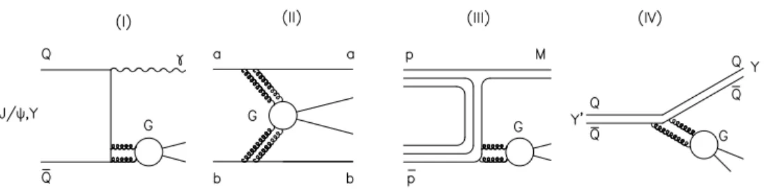
3.1.2. Glueball decays. Bound gg states (“gluonia”) decay through a two gluon intermediate state where several mechanisms can be envisaged [35] (see figure 3)
a) gb → gg → qq ¯ q ¯
′q
′→ M M
′(21a)
b) gb → gg → gggg → η(η
′) η(η
′) or → gb gb (21b) c) gb → gg → qq ¯ → qq ¯ q ¯
′q
′→ M M
′(21c) In the decay rates of these processes the ratio of amplitudes
R ≡ h s¯ s | V | g i / h d d ¯ | V | g i (22)
‡ Previously, a favoured value was quoted asφps= 37.4◦, θps=−17.3◦[3].
Figure 2. Couplings γij2 for isoscalar (q¯q) meson decays as function of mixing angle αas in (15) forSU(3)f l symmetry (ρ= 1) from table 3 with rG = 0 for φps= 37.4◦ (figure from [35]).
Figure 3. Processes contributing to gluonium decay (21a-21c) (figure from [35]).
Table 3. Couplings γij2 for decay of an I = 0 meson f0 with mixed (q¯q) and (gg) components [35, 36]; flavour mixing anglesαas in (15), φ≡φps as in (17a); glueball decay according to (21a) [35]; SU(3)f l breaking parameters ρ, R as defined in (12) and (22); weights cij included in γij2; decay couplings g2ij = g2γij2/4 for (qq) and¯ rG =p
3/(2 +R2)G/g for (gg) withg, Gfrom (24) (based on [36, 37]).
decay channel couplingsγij2 for|f0i= cosφG|q¯qi+ sinφG|ggi weights
ππ 3(cosα+rG)2 3
KK¯ (ρcosα−√
2 sinα+ 2rG)2 4
ηη (cosαcos2φ−√
2ρsinαsin2φ+rG(cos2φ+R2sin2φ))2 1 ηη′ 2 cos2φsin2φ(cosα+√
2ρsinα+rG(1−R2))2 2 η′η′ (cosαsin2φ−√
2ρsinαcos2φ+rG(sin2φ+R2cos2φ))2 1
appears for the q q ¯ production from a gluon, where R
2= 1 for SU (3)
f lsymmetry. For the decay of a mixed state
| f
0i = cos φ
G| q q ¯ i + sin φ
G| gg i (23) with | q q ¯ i mixed as in (15) and | gg i decaying as in (21a) into pairs of pseudoscalars we write the decay couplings as [37]
g
ij= g d
ijq¯q+ G d
ijgg; g = g
0cos φ
G, G = G
0sin φ
G. (24) The couplings γ
ij2for the decay of the mixed state with the factor g
2/4 taken out and with r
G= p
3/(2 + R
2) G/g are given in table 3. For the glueball decay with flavour symmetry (R = 1) one finds from the term with r
G∝ G the reduced partial widths γ
2ijγ
ij2(gb → ππ : K K ¯ : ηη : ηη
′: η
′η
′) = 3 : 4 : 1 : 0 : 1 (25) according to the statistical weights.
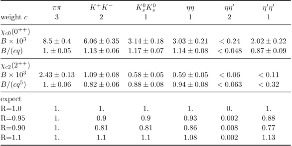
The two-gluon intermediate process also dominates the decays of scalar heavy quark, c¯ c, bound states with C parity C = +1 like χ
cin the perturbative analysis and one expects decay rates as in (25). An update of this test for spin J = 0, 2 charmonia χ
c0, χ
c2[35] is carried out in table 4. We list the measured branching ratios B into pairs of pseudoscalars according to the PDG [4], where recent contributions come from CLEO [43] and BES [44]. From the model (but without dynamical formfactor F
ij(q
2), i.e. β → ∞ ) one expects B ∝ c | M |
2q
2ℓ+1. In table 4 we also show B after division by cq
2ℓ+1, and after normalization to that value for the ππ decay. These data are to be compared with the model predictions for | M |
2= γ
2/c in table 3 for (gg), i.e. for g/G → 0, where recall g and G are given by (24). These expectations are given in table 4 as well for different values of the strange quark parameter R in (22). We observe, that the expectations from SU(3)
f lsymmetry (R = 1) are fulfilled for all decay processes of χ
c0,2within 10 - 20% (only the upper bound for χ
c2→ η
′η
′is a bit low). So there is no strong need for the additional gluonic processes (21b) affecting η, η
′; nor is there any strong need for dynamical form factors F
ij(q
2); the weakness of angular momentum barrier factors (of Blatt-Weisskopf type) may be due to the small radius of charmonium states of O(1/m
c).
Looking at the substructures at the 10% level we note that for the tensor state χ
c2the observed values for B/(cq
5) would prefer a slightly reduced R & 0.9. In case of the decays of the scalar χ
c0values of B/(cq) for kaons are slightly enhanced by 10- 20%. This effect could be a remote consequence of the chiral enhancement in scalar decays discussed above from the contribution of the intermediate process gg → q¯ q as considered for scalar glueballs in (21c) (the argument is also applicable for a decaying scalar c¯ c state). The effect can be simulated by choosing R > 1 and we give in the last line of table 4 the predictions for R = 1.1 which would fit the data for χ
c0generally better.
A modification of the SU (3)
f lsymmetry for decay rates (with R = 1 in table 4) is
expected in schemes which include state mixing at hadronic scales and mixing of decay
Table 4. Branching ratiosB of χc0(3415) (0++) and χc2(3556) (2++) into pairs of pseudoscalars; also B/(cq) or B/(cq5) resp. with charge weight c and momentum q after normalization to the value forππ(data as listed in [4]), together with the resp.
theoretical expectations |M|2 = γij2/c for process gg in table 3 for different strange quark parametersR (mixing angleφps≈37.4◦ forη, η′).
ππ K+K− Ks0Ks0 ηη ηη′ η′η′
weightc 3 2 1 1 2 1
χc0(0++)
B×103 8.5±0.4 6.06±0.35 3.14±0.18 3.03±0.21 <0.24 2.02±0.22 B/(cq) 1.±0.05 1.13±0.06 1.17±0.07 1.14±0.08 <0.048 0.87±0.09 χc2(2++)
B×103 2.43±0.13 1.09±0.08 0.58±0.05 0.59±0.05 <0.06 <0.11 B/(cq5) 1.±0.06 0.82±0.06 0.88±0.08 0.94±0.08 <0.063 <0.32 expect
R=1.0 1. 1. 1. 1. 0. 1.
R=0.95 1. 0.9 0.9 0.93 0.002 0.88
R=0.90 1. 0.81 0.81 0.86 0.008 0.77
R=1.1 1. 1.1 1.1 1.08 0.002 1.13
constants at short distances [42]; in that case the ratios of the χ
cdecay rates deviate considerably from unity, for example B (χ
c0→ ηη)/B(χ
c0→ π
0π
0) = 1.9 and the same follows for the ratio (η
′η
′)/(π
0π
0). The data appear to be closer to the conventional meson state mixing approach as seen in table 4.
The remarkable success of the simple scheme based on SU (3)
f lsymmetry with phase space correction for decays into the same nonets suggests further tests with other nonets in the search for extra gluonic states, as will be discussed in section 10.
3.2. Enhanced and suppressed glueball production
Not only the decay, also the production properties are characteristic for the intrinsic structure of a hadronic state [45, 46].
3.2.1. Gluon-rich processes. There are processes which provide a “gluon rich”
environment with enhanced probability for glueball production, see figure 4 for examples.
These processes have been extensively explored experimentally in the past [5, 7]. We give here a survey first over different processes and come back to specific problems later:
(i) Radiative J/ψ or Υ decay: In the perturbative approach the (c¯ c) or other heavy quarkonium J
P C= 1
−−bound states decay predominantly through (Q Q) ¯ → 3g.
Alternatively, the radiative decay (Q Q) ¯ → γ + (2g) is possible with formation of
an intermediate gluonium (gg) state ((Q Q) ¯ → γ + gb).
Figure 4. Processes favouring glueball G production, where J/ψ and Υ are respectively the lowest massc¯candb¯bmesons withJP C= 1−−.
(ii) Central production of mesons: In double diffractive high energy processes the incoming hadrons scatter with small momentum transfers and carry on the initial valence quarks. In Regge theory this process is dominated by “double Pomeron exchange”. If the Pomeron is viewed as a gluon dominated object then glueball production is enhanced in this reaction (pp → p gb p). The different contributing processes within QCD have been discussed in [47].
(iii) p¯ p annihilation: The annihilation of quarks may proceed through intermediate gluons and the formation of glueballs (p¯ p → gb + M ).
(iv) Decay of excited heavy quarkonium Y
(n)to ground state Y : In the example Y
(n)→ Y + X the hadrons X are emitted from intermediate gluons and therefore could be formed through an intermediate glueball.
(v) Decay of heavy quark b → sg: This QCD process (through “penguin” diagram) may hadronize involving a glueball according to B → Kgb [48].
(vi) Leading particle in gluon jet: In analogy to the fragmentation of the primary quark q of a q-jet into an energetic meson M (q¯ q
′) which carries q as valence quark, there may be the fragmentation of the primary gluon of a gluon jet into an energetic meson M (gg) which carries the initial gluon as valence gluon g → gb + X (section 9).
3.2.2. Suppression of glueballs in γγ processes. Having neutral constituents a glueball couples to photons only through loop processes and then it is suppressed in γγ reactions.
3.3. Supernumerous states among q q ¯ nonets?
Mesons with light quark constituents (u, d, s quarks) are classified in nonets of 3 × 3 states (octet+singlet). A well known example is the pseudoscalar nonet of lowest mass with π, K, η near flavour octet and η
′near singlet. It is the aim of meson spectroscopy to establish the appropriate classification of mesons. They should fit into nonets of q q ¯ states - possibly, there are also exotic states like tetra-quark qq q ¯ q ¯ or hybrid q qg ¯ states.
If there are glueballs in addition there should be supernumerous states which do not fit
into a nonet classification of the meson spectrum.
4. Spectroscopy of scalar mesons: q q ¯ nonets mixing with glueballs
In the scalar sector different schemes have been proposed for a spectroscopy with glueballs for the mesons below 2 GeV including the isoscalars of (1).
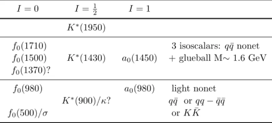
Table 5. Spectroscopy with glueballs, route 1: glueball near 1500 MeV.
I= 0 I= 12 I= 1 K∗(1950)
f0(1710) 3 isoscalars: q¯qnonet
f0(1500) K∗(1430) a0(1450) + glueball M∼1.6 GeV f0(1370)?
f0(980) a0(980) light nonet K∗(900)/κ? q¯q or qq−q¯¯q
f0(500)/σ orKK¯
4.1. Route 1: (q q) ¯ nonet - glueball mixing around 1500 MeV
Lattice QCD in quenched approximation predicts the lightest glueball in the mass range around 1600 MeV (see section 2.2). The discovery of the rather narrow f
0(1500) in p p ¯ annihilation by the Crystal Barrel Collaboration [49] and by GAMS [50] suggested at first the possibility of a gluonic state. A closer inspection of decay mechanisms and branching ratios led Amsler and Close [35] to propose a mixing scheme including f
0(1370) and f
0(1710) with a gluonic component as well § . In table 5 we list the meson states ordered according to mass and isospin. Between 1.0 and 1.9 GeV we find the states fitting into a q q ¯ nonet but with one supernumerous isoscalar which suggests the presence of a glueball.
With more experimental results available and with further development of models various mixing schemes for the three isoscalars have been proposed (for a further discussion, see [7]). As an example, we present the result [51] which includes data for γγ processes. The physical mass states f
0(m
i) are decomposed into the q¯ q and gg states or, alternatively, into the SU (3) eigenstates | 1 i = ( | u¯ u i + | d d ¯ i + | s¯ s i )/ √
3 and
| 8 i = ( | u¯ u i + | d d ¯ i − 2 | s¯ s i )/ √
6 and gluonium | gg i
| f
0(1370) i
| f
0(1500) i
| f
0(1710) i
=
0.86 0.13 − 0.50 0.43 − 0.61 0.61 0.22 0.76 0.60
.
| n n ¯ i
| s¯ s i
| gg i
=
0.78 0.39 − 0.50 0.00 0.75 0.61 0.62 − 0.49 0.60
.
| 1 i
| 8 i
| gg i
(26) One observes that in this scheme f
0(1500) is a mixture only of octet q q ¯ and glueball; the glueball component is distributed over all three f
0states (last column in mixing matrix) with about equal amounts. In alternative schemes either f
0(1500) can be dominantly gluonic [52] or f
0(1710) while f
0(1370) is near singlet [53, 52].
§ In the scheme [35] the existence of the heavy state (nowf0(1710)) actually has been predicted.
A possible problem with this mixing scheme are the doubts related to the very existence of f
0(1370). This resonance is included in global fits of parametric model amplitudes to a variety of channels but it is not seen in any model independent bin-by- bin phase shift analysis. The PDG under this entry does not provide any established result on branching ratios or ratios thereof - contrary to the well established nearby f
0(1500). We come back to this problem in more detail in section 7.
The light scalar mesons below 1 GeV can be grouped into another nonet (see table 5) which includes the broad states f
0(500)/σ and K
∗(800)/κ, besides the narrow f
0(980) and a
0(980). This meson nonet can been built from q q ¯ as usual, see, for example [54, 55, 56]. Alternatively, it can be given a substructure of diquarks (qq − q ¯ q) according ¯ to the scheme by Jaffe [57] within the MIT bag model where the nonet is constructed as the direct product of the anti-triplet of diquarks (ud, us, ds) and the triplet of anti- diquarks (¯ u d, ¯ u¯ ¯ s, d¯ ¯ s). This construction explains naturally the ordering in mass of the states where a
0, f
0have two, κ has one and σ has no s(¯ s) quark constituent
a
+= [su] [¯ s d], ¯ f
0/a
0= ([su] [¯ s u] ¯ ± [sd] [¯ s d])/ ¯ √
2, a
−= [sd] [¯ s¯ u]
κ
+= [su] [¯ u d], ¯ κ
0= [sd] [¯ u d], ¯ κ ¯
0= [ud] [¯ s d], ¯ κ
−= [ud] [¯ s u] ¯ (27) σ = [ud] [¯ u d] ¯
Various applications of the 4-quark model for the light scalars have been considered for decay and production processes, in particular with photons [58, 59]. A picture of these scalar mesons as a mixture of tetra-quark states (dominating in the light mesons) and heavy (q¯ q) states (dominating the heavier mesons) has been proposed in [60] based on an instanton induced effective Lagrangian theory. The mixing between the mass eigenstates f
0and σ and the ideally mixed states in (27) is typically assumed small to be consistent with the near mass degeneracy of f
0and a
0. For example, the corresponding mixing angle is | ω | < 5
◦in [60].
The light scalar mesons can be established by the motion of phase shifts through 90
◦in the appropriate two-body processes, except for the κ with a phase in Kπ-scattering staying below 40
◦(see section 5.2).
4.2. Route 2: light glueball around 1 GeV
The QCD results discussed above do not allow a definitive conclusion about the mass and properties of the lightest scalar glueball. A light glueball near 1 GeV is obtained from QCD sum rules; based on low energy theorems also a large width is suggested which points to f
0(500), sometimes also referred to as f
0(500 − 1000) according to the heavier Breit-Wigner mass of ∼ 1000 MeV (see below and section 5.1.1). A light glueball near 1000 MeV is also expected from certain lattice calculations [21] (see section 5.1.1), both states f
0(500 − 1000) or f
0(980) are possible candidates.
In view of the theoretical ambiguities at the end of the 90’s, a largely
phenomenological approach to light scalars including a glueball has been pursued by
Minkowski and Ochs [61] without reference to the above specific QCD results. General properties, especially mixing patterns are studied basing on an effective action for sigma variables [62]. The lightest q¯ q nonet is constructed from the list of well established resonant states, see table 6. In particular, the existence of f
0(1370) as an extra state has not been accepted: the peaks appearing in the ππ mass spectrum have been interpreted as caused by a broad object centered around 1 GeV interfering destructively with the narrow resonances f
0(980) and f
0(1500) (“red dragon” phenomenon). This broad object has been related to f
0(500): after separation of f
0(980) the ππ elastic phase shifts pass 90
◦near 1000 MeV and can be represented locally by a “Breit-Wigner” resonance. A typical fit for “f
0(1000)” yields (see also [63])
M
BW≈ 1000 MeV, Γ
BW≈ 700 MeV. (28)
The determination of the amplitude pole from the phase shifts is non-trivial and we come back to this question in section 5.1.1.
The lightest q¯ q nonet in that scheme includes the isoscalars f
0(980) and f
0(1500) with a mixing similar to η
′− η. This has been motivated by the observed decay rates J/ψ → ω, φ + X which project out the strange and non-strange quark components of X k and are found comparable for X = η
′and X = f
0(980). According to PDG [4] (in units of 10
−4):
B(J/ψ → ωη
′) = 1.82 ± 0.21; B(J/ψ → φη
′) = 4.0 ± 0.7 (29) B(J/ψ → ωf
0(980)) = 1.4 ± 0.5; B(J/ψ → φf
0(980)) = 3.2 ± 0.9 (30) We write the flavour mixing of these scalar mesons as
| f
0(980) i = sin φ
sc| n n ¯ i + cos φ
sc| s¯ s i , (31)
| f
0(1500) i = cos φ
sc| n n ¯ i − sin φ
sc| s¯ s i , (32) or inversely
| n¯ n i = sin φ
sc| f
0(980) i + cos φ
sc| f
0(1500) i (33)
| s¯ s i = cos φ
sc| f
0(980) i − sin φ
sc| f
0(1500) i . (34)
k It is assumed that the “singly disconnected diagram”, where the qq¯is produced in a single loop through one intermediate gluonic exchange, dominates over the “doubly disconnected diagrams” [40].
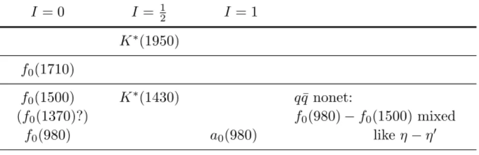
Table 6. Spectroscopy with glueballs, route 2: light glueball around 1 GeV.
I= 0 I=12 I= 1
K∗(1950) f0(1710)
f0(1500) K∗(1430) q¯qnonet:
(f0(1370)?) f0(980)−f0(1500) mixed
f0(980) a0(980) likeη−η′
(K∗(900)/κ?)
f0(500)/σ light glueball m∼1 GeV
For estimates, the flavour composition | u¯ u, d d, s¯ ¯ s i has been approximated by η
′, f
0(980) ↔ | 1, 1, 2 i / √
6; η, f
0(1500) ↔ | 1, 1, − 1 i / √
3. (35)
The octet formed from a
0(980), K
0∗(1430) and f
0′≡ f
0(1500) is found to follow the Gell-Mann-Okubo mass relation (using masses 984.7, 1412 and 1507 MeV)
m
2(f
0′) = m
2(a
0) +
43(m
2(K
0∗) − m
2(a
0)) (36)
2.271 = 0.970 + 1.365 = 2.335 [GeV
2] (37)
within a few percent.
The correspondence η
′↔ f
0(980) and η ↔ f
0(1500) is also characteristic of the
“Bonn quark model” [64, 65] and the model of Nambu-Jona-Lasinio type [66] which include instanton interactions with axial U(1) symmetry-breaking [67]; these models explain the reversed mass differences between the octet and singlet states in the scalar and pseudoscalar nonets.
The extra state f
0(500 − 1000) is then supernumerous and is taken as glueball. This identification is supported at first view by the observation of this state in all ”gluon rich”
processes (i)-(v), with the possible exception of J/ψ → γπ
0π
0which is difficult to select from background [68]. ¶ Other results within this scheme are presented in [61] and on the appearance in D, D
sand B decays in [70] and [48]. The κ meson is not required in this scheme. Further discussion follows in the subsequent sections on f
0′s.
4.3. Route 3: two supernumerous states, broad glueball f
0(1200 − 1600)
A global description of processes with mesonic final states ππ, K K, ηη, ηη ¯
′, 4π with J
P C= 0
++in the mass range 280 -1900 MeV in terms of a K matrix and also using a dispersion relation method has been presented by Anisovich et al. [71] (earlier work in [36, 37]). Data from ¯ pp, pn ¯ annihilation into three mesons and meson pair production in πp collisions have been included in a global fit. The appropriate mixing angle φ is determined for each resonance from their decays (following table 3) where the glueball decay is “flavour blind” with a modification from strange quark suppression. The two isoscalar states in a nonet are orthogonal in flavour space and the mixing angles of the respective states should fulfill
φ
(I)− φ
(II)= ± 90
◦. (38) The results of the fits suggested the classification of the isoscalar states as in table 7 with two q q ¯ nonets and one broad state f
0(1200 − 1600) (width Γ = 1100 ± 140) identified as glueball. Alternatively, one could exchange the roles of f
0(1300) and f
0(1200 − 1600) which are both near flavour singlet. The σ meson is another extra state and it is related to a confinement singularity of the q q ¯ potential.
¶ Preliminary data from BES-III suggest a contribution fromf0(500) centered at low masses around 500 MeV [69].
Table 7. Spectroscopy with glueballs route 3: two supernumerous states.
[f0(980), f0(1300)] [f0(1500), f0(1750)] qq¯nonets
f0(1200−1600) f0(500)/σ glueball, extra state
![Figure 1. Mass spectrum of glueballs (in GeV on r.h.s.) for different quantum numbers P C according to the quenched lattice calculations (figure from [18]).](https://thumb-eu.123doks.com/thumbv2/1library_info/4023854.1541955/6.918.278.606.128.511/figure-spectrum-glueballs-different-quantum-according-quenched-calculations.webp)
![Table 3. Couplings γ ij 2 for decay of an I = 0 meson f 0 with mixed (q¯ q) and (gg) components [35, 36]; flavour mixing angles α as in (15), φ ≡ φ ps as in (17a); glueball decay according to (21a) [35]; SU (3) f l breaking parameters ρ, R as defined in (1](https://thumb-eu.123doks.com/thumbv2/1library_info/4023854.1541955/13.918.218.771.979.1112/couplings-components-flavour-glueball-according-breaking-parameters-defined.webp)
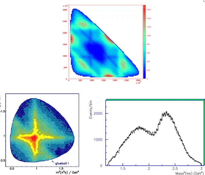
![Figure 5. Phase shifts of elastic scattering, Left: ππ phase shifts from Dispersion Relations [100] and from resonance fit to CM-I data [101] (f 0 (980) + background [102]); Middle: Kπ phase shifts (K 0 ∗ (1430) + background [103, 104]); Right: Kπ phase sh](https://thumb-eu.123doks.com/thumbv2/1library_info/4023854.1541955/26.918.123.767.136.340/figure-elastic-scattering-dispersion-relations-resonance-background-background.webp)
![Figure 7. Upper part left: Dalitz plot for p¯ p → π 0 ηη at √ s = 2.0 GeV (Crystal Barrel); right: mass 2 (ηη) spectrum (figures from [128])](https://thumb-eu.123doks.com/thumbv2/1library_info/4023854.1541955/33.918.139.719.134.406/figure-upper-dalitz-crystal-barrel-right-spectrum-figures.webp)