EQUATIONS AND SCALING
AT LOW LATITUDES
The governingequationsofatmospheric andoceanicmotionare intrinsically
complicated, a reection of the myriad of time and space scales they repre-
sent. Therefore, in order to study a specic phenomenon it is desirable to
simplify the equations by a scale analysis, removing those terms which are
unimportant for the phenomenon in question. The scaling to be described
here isincomplete,but isaimed atcomparing thedominantprocessesatlow
and higher latitudes. A scale analysis for midlatitude synoptic systems is
described in DM, Chapter 3.
2.1 The governing equations on a sphere
The basic equations for the motion of adry atmosphere are
Du
Dt
= rp+g ^ u+F; (2.1)
D
Dt
= ru; (2.2)
c
p D
Dt ln=
Q
T
; (2.3)
p=R T: (2.4)
The rst three represent the conservation of momentum, the conserva-
tion of mass and the conservation of energy (rst law of thermodynamics),
respectively; the lastisthe equation ofstate. The variables u,p, ,T and
andQrepresentthe(three-dimensional)uidvelocity,total pressure,density,
temperature, potentialtemperature, and diabaticheating rate,respectively;
F represents viscous and or turbulentstresses, and g isthe eective gravity.
The potentialtemperatureisrelatedtothetemperatureandpressure by the
formula=T(p
=p)
, wherep
= 1000 mband =0.2865.
Theshapeof theearthssurface isapproximatelyanoblatespheroid with
an equatorial radius of 6378 km and a polar radius of 6357 km. The sur-
face is close to a geopotential surface, i.e. a surface which is perpendicular
to the eective gravity (see DM, Chapter 3). As far as geometry is con-
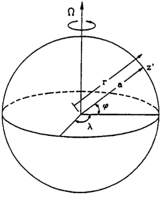
cerned the equations of motion can be expressed with suÆcient accuracy
in a spherical coordinate system (;;r), the components of which repre-
sent longitude, latitudeand radialdistance fromthe centre of the earth (see
Fig. 2.1). The coordinate system rotates with the earth at an angular rate
=jj=7:29210 5
rads 1
. Animportantdynamicalrequirementinthe
approximation to a sphere is that the eective gravity appears only in the
radial equation of motion, i.e. we regard spherical surfaces as exact geopo-
tentials so that the eective gravity has no equatorial component. Further
details are found inGill(1982; 4.12).
Alternatively,theequationsmaybewrittenincoordinates(;;z),where
is the longitude of a point, the latitude, and z is the height above the
earths surface (or more precisely the geopotential height). Note that r =
a +z, where a is the earths radius. Since the atmosphere is very shallow
compared with its radius (99% of the mass of the atmosphere liesbelow 30
km,whereas a=6367km),wemayapproximate rby aand replace@=@r by
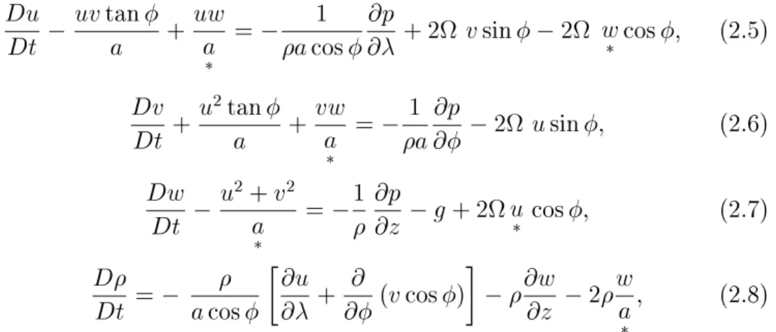
@=@z. In (;;z) coordinates, the frictionless forms of Eqs. (2.1) and (2.2)
are (Holton,1979, p 35)
Du
Dt
uvtan
a +
uw
a
=
1
acos
@p
@
+2 vsin 2 w
cos; (2.5)
Dv
Dt +
u 2
tan
a +
vw
a
= 1
a
@p
@
2 usin; (2.6)
Dw
Dt u
2
+v 2
a
= 1
@p
@z
g+2 u
cos; (2.7)
D
Dt
=
acos
@u
@ +
@
@
(vcos)
@w
@z 2
w
a
; (2.8)
whereu=a cos d
dt i+r
d
dt j+
dz
dt
k=ui+vj+wk. Hereu;vandwrepresentthe
eastward,northwardandverticalcomponentsofvelocity,and D
@
+ur,
Figure2.1: The (;;z) coordinatesystem
is the total-, or Lagrangian-,or material-derivative,following anairparcel.
The terms with an asterisk beneath them willbe referredto later.
2.2 The hydrostatic equation at low latitudes
In Chapter 1 we discussed the enormous diversity of motion scales which
exists inlowlatitudes. Weexplore nowtherange ofscales forwhich wemay
treat the motionas hydrostatic.
Tocarryoutascalingof(2.7)itisconvenienttodeneareferencedensity
and pressure,
0
(z) and p
0
(z), characteristic of the tropical atmosphere and
to dene a perturbation pressure p 0
as the deviation of p from p
0
(z). Then
g in Eq. (2.7) must be replaced by the buoyancy force per unit mass,
= g(
0
(z) )=, and p may be replaced by p 0
in Eqs. (2.5) and (2.6).
Detailsmaybefound inDM, Ch. 3. Omittingprimes,(2.7) may bewritten
Dw
Dt +
1
@p
@z
= u
2
+v 2
a
+2ucos: (2.9)
ToperformthenecessaryscaleanalysisweletU;W;L;D;Æp;and rep-
resent typical horizontal and vertical velocity scales, horizontaland vertical
length scales, a pressure deviation scale, a buoyancy scale and a time scale
for the motion of aparticular atmospheric system. The terms in (2.9) then
have scales
W
Æp
D
U 2
a
2U (2.10)
For a value of Æp 1 mb (10 2
Pa) over the troposphere depth (20 km),
Æp=(D)10 2
( 1:02:010 4
)=0:510 2
ms 2
. AlsoforU 10ms 1
,
10 5
s 1
and a610 6
m,the lasttwoterms are of the order of 10 4
and can be neglected.
The principal question is whether the vertical acceleration term can be
neglected compared with the vertical pressure gradient per unit mass. To
investigate this consider
Dw
Dt
=
1
@p
@z
W
=
1
Æp
D
: (2.11)
We obtain an estimate for Æp from the horizontal equation of motion (2.1).
This yields two possible scales, depending on whether the motion is quasi-
geostrophic, i.e. 1= <<f,or whether inertial eects predominate, 1= >>
f. Inthe latter case (f <<1),
ÆpP
1
=LU=;
while in the former case (1<<f)
ÆpP
2
=LUf:
If 1= = f, then, of course, Æp P
1
= P
2
. Withthe foregoing scales for
P we can calculatethe ratio in (2.11). Using P
1
we nd that
W
= 1
P
1
D
= W
U D
L
Thus in the high frequency limit (f << 1), hydrostatic balance will
occur if W << U and/or D=L << 1, provided that the other ratio is no
morethanO(1). Asweshallsee later,thisallowsgravitywavestobetreated
hydrostatically,but the approximation isnot validfor cumulus clouds.
In the low frequency limit (1<<f)we use P
2
, and obtain
W
= 1P
2
=
W D
:
Now, even if W U and D L, the hydrostatic approximation is justied
provided 1<< f;whichwasthe approximationthatallowedustoobtainP
anyhow. For synoptic-scale (L 10 6
), or planetary-scale (L a) motions,
for both of which L >> D, the hydrostatic approximation is valid even if
1= f,and thereforeasf decreases towards theequator. Thuswearewell
justied in treatingplanetary motionsas hydrostatic.
Wemust be careful, however. Wenote that (2.5) hasa componentof the
Coriolis forcethatis amaximum atthe equator, i.e. although2vsin!0
as !0, 2wcos!2w. But in invoking the hydrostatic approximation
we neglectthe term2ucos in(2.7). Thusforming the totalkinetic energy
equation with our new hydrostatic set we will produce an inconsistency. It
appears inthe following manner. Multiplying (2.5) u, (2.6) v and (2.7)
w and adding, we obtain
D
Dt
1
2 u
2
+v 2
+w 2
= 1
u
acos
@p
@ +
v
a
@p
@ +w
@p
@z
gw: (2.12)
We notice that all geometric terms and Coriolis terms have vanished by
cancellationbetween theequations. Thisisasitshouldbeasthesetermsare
products of the geometryorare a consequenceof Newtons secondlawbeing
expressed inanacceleratingframeofreference. Thatis,thetermswould not
appear as forces in aninertial frameand may not change the kinetic energy
of the system.
Theproblemis: ifwemaketheassumptionthatthe systemishydrostatic
andnotethatforlargescaleow,jwj<<juj;jvj,thenthetotalkineticenergy
may bewritten as
1
2 D
Dt u
2
+v 2
= 1
u
acos
@p
@ +
v
a
@p
@
2uwcos
u 2
+v 2
a
w
:
(2.13)
The last term in square brackets represents a ctitious or spurious en-
ergy source that arises fromthe lack of consistency in scaling the system of
equations. Sinceeachequationis interrelatedtothe others, itisincorrect to
scale one without consideration of the others. Therefore, if the hydrostatic
equation is used, energetic consistency requires that certain curvature and
Coriolistermsmustbeomittedalso. Thesearethetermsmarkedunderneath
by a star in Eqs. (2.5) - (2.8). Similar considerationsto these are necessary
when "sound -proong" the equations (see e.g. ADM, Ch. 2).
The hydrostatic formulation of the momentum equations with friction
terms included then becomes
Du
Dt
=
1
acos
@p
@ +
2+ u
acos
vsin+F
; (2.14)
Dv
Dt
= 1
a
@p
@
2+ u
acos
usin+F
; (2.15)
0= 1
@p
@z
g: (2.16)
The need to neglect certain terms in the u and v equations to preserve
energeticconsistencyhasnotbeenalwaysappreciated. Manyearlynumerical
models, which were hydrostatic, could not conserve the total energy (i.e.
kinetic and potentialenergy). The problem was traced to the inconsistency
noted above.
2.3 Scaling at low latitudes
We consider now a more formal scaling of the hydrostatic equations in the
vector form
@
@t
+Vr
h
V+w
@
@z
V+fk^ V = (1=) r
h
p (2.17)
0= 1
@p
@z
g (2.18)
@
@t
+Vr
h
+r
h V+
@
@z
(w)=0 (2.19)
@
@t
+Vr
h
ln+w
@
@z
ln =Q=(c
p
T): (2.20)
Here V isthe horizontalwind vector, wthe verticalvelocity componentand
r
h
is the horizontal gradient operator. We recognize that perturbations of
pressure and density from the basic state p
0 (z),
0
(z) are relatively small,
but seektoestimatetheir sizesforlow-andmiddle-latitudescalingsinterms
of ow parameters.
We dene a pressure height scale H
p
such that 1=H
s
= (1=p
0 )(dp
0
=dz)
and note that, using the hydrostatic equation for the basic reference state,
H
p
=p
0
=g
0
. Withquasi-geostrophicscalingappropriatetomiddle-latitudes,
Eq. (2.17) gives Æp
0
fUL,whereupon
Æp
p
0
fUL
gH
p
= F
2
R o
Ro<<1
(2.21)
where R
o
= U
fL
is the Rossby number,
and
F = U
(gHp) 1=2
is aFroude number.
Note that (2.21) is satised even if R o 1, because Æp
0
fUL then
provides the same scale asthe inertialscale Æp
0 U
2
.
Hydrostatic balance expressed by (2.18) implies hydrostatic balance of
the perturbation from the basic state, i.e. @p 0
=@z = g 0
, whereupon it
follows that Æp=D gÆ,and therefore
Æ
0
Æp
gD
0
Æp
p
0
H
s
D
Æp
p
0
= F
2
R o
Ro<<1
; (2.22)
assuming DH
p .
Finally,since fromthe denitionof ,(1 )lnp =ln+ln +constant,
Æ
0
Æp
p
0
F 2
R o
Ro<<1
: (2.23)
Typically, g 10 ms 2
, H
p
10 4
m whereupon, for U 10 ms 1
,
f 10 4
s 1
(a middle-latitudevalue), R o = 0:1 and F 2
= 10 3
. It follows
that in middlelatitudes,
Æ
0
Æp
p
0
Æ
0 10
2
; (2.24)
conrming that for geostrophic motions, uctuations in p, and may be
treated assmall.
At low latitudes, f 10 5
s 1
so that for the same scales of motion as
above, R o=1. In this case, advection terms in (2.17) are comparable with
the horizontal pressure gradient. However, as we have seen, the foregoing
scalings remainvalidfor R o1and therefore
Æ
0
Æp
p
0
Æ
0 10
3
: (2.25)
Accordingly, we can expect uctuations in p, and to be an order of
magnitude smaller inthe tropics than inmiddlelatitudes. The comparative
rapidity of the adjustment of the tropical motions to a pressure gradient
imbalance; the adjustment being less constrained by rotational eects than
at higher latitudes.
Consider now the adiabaticform of (2.20), i.e., put Q =0. The scaling
of this equationimplies that
U
L Æ
0
W
1
0 d
0
dz :
Using(2.23) and dening
N 2
= g
0 d
0
dz
;
where N is the buoyancy frequency and,
R i= N
2
H 2
p
U 2
;
is a Richardson number, we have
U
L F
2
R o
W
N 2
g
; mathrmor W UD
L 1
R oR i
; (2.26)
anestimatethatisvalidforR o=1. Itfollowsthat,forthesamescalesofmo-
tion and in the absence of convective processes of substantial magnitude, we
may expect the vertical velocity inthe equatorialregions tobe considerably
smaller than inthe middlelatitudes. Forexample, fortypicalscales U =10
ms 1
, D = 10 km, L = 1000 km, H
p
= 10 km, N = 10 2
s 1
, R i = 10 2
and W =10 3
=R o ms 1
. In the tropics,R o 1 sothat (2.26) would imply
vertical velocities onthe order of 10 3
ms 1
, which isexceedingly tiny.
2.4 Diabatic eects, radiative cooling
Weshallseethatinthe tropicsitisimportanttoconsiderdiabaticprocesses.
We consider rst the diabatic contribution in regionsaway from active con-
vection so that the net diabatic heating is associated primarily with radia-
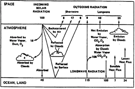
tive cooling to space alone. Figure2.2 shows the annual heat balance of the
earthsatmosphere. Ofthe 100units ofincomingshortwave(SW) radiation,
31 units are reected while the atmosphere radiates 69 units of long wave
(LW) radiationtospace. Accordingly,atthe outer limitsof theatmosphere,
there exists radiative equilibrium. Altogether 46 units of SW radiation are
absorbed atthe surface. The surface emits115 units of radiationinthe long
wave part of the spectrum, but 100 units of this are returned from the at-
mosphere. It is clear that, on average, there is a net radiative cooling of the
atmosphere, amounting to 31 units, or 31% of the available incident radia-
tion. On average, this cooling is balanced by a transfer of sensible heat (7
units)and latentheat (24units)totheatmospherefromearthssurface. The
incoming solar radiation of 1360 Wm 2
(the solar constant) intercepted by
the earth(a 2
1360)W isdistributed,whenaveragedoveraday orlonger,
over anarea 4a 2
(see Fig. 2.3).
Figure 2.2: Schematic representation of the atmospheric heat balance. The
units are percent of incomingsolar radiation. The solar uxes are shown on
theleft-handside,andthelongwave(thermalIR)uxesareontheright-hand
side (fromLindzen,1990).
Figure2.3: Distribution of solar radiationoverthe earthssurface.
As discussed above, the atmosphere loses heat by radiation over 1 day
or longer at the rate Q = 0:31 0:251360 W/m 2
. In unit time, this
corresponds to a temperature change T given by Q = c
p
MT, where
M is the mass of a columnof atmosphere 1 m 2
in cross-section. Since M =
(mean surface pressure)/g, we nd that
T =
0:310:251360243600
10051:01310 4
0:9K/day:
Actually, the rate of cooling varies with latitude. From the surface to
150 mb (i.e. for 85% of the atmospheres mass), T 1:2 K/day from
0 30 Æ
lat., 0:88 K/day from 30 - 60 Æ
lat., and 0:57 K/day from 60 -
90 Æ
lat. The stratosphereandmesospherewarm alittleonaverage,but even
together they have relativelylittlemass.
The estimate(2.25) suggests that for synoptic scale systems in the trop-
ics, we can expect potential temperature changes associated with adiabatic
changes of no more than a fraction of a degree. The estimate (2.26) shows
thatassociatedverticalmotionsareontheorderDU/(LRi)whichistypically
10 4
10(10 6
(10 4
10 8
10 2
))10 3
ms 1
.
In contrast, radiativecoolingat the rate Q=c
p
= 1:2K/day would lead
to asubsidence rate which we estimated from(2.20) as
WN 2
=g (Q=c
p )=T;
whereupon
W
g
N 2
1:2
300
1
243600
= 0:5cm/sec:
It follows that we may expect slow subsidence over much of the tropics and
that the vertical velocities associated with radiative cooling are somewhat
larger than those arising fromsynoptic-scale adiabaticmotions.
We consider nowthe implications of the foregoingscalingon the vertical
structureoftheatmosphere. Theverticalcomponentofthevorticityequation
corresponding with (2.17) and (2.18) is
@
@t
+Vr
A
+
rV+w
@
@z +k
B
rw^
@V
@z
+Vrf
C
+f r
D V
=k^
(1=) r^(1=)
E rp
(2.27)
We compare the scales of eachterm in this equation with the scale for term
Table 2.1: Ratio of terms inEq. (2.27).
Term A B C D E
Generally 1
L
U W
D
2
U L
2
a cos
L
U W
D 1
Ro F
2
Ro 2
Midlatitudes
R o<<1
1 1
RiRo
( " )
1
RiRo 2
F 2
Ro 2
Lowlatitudes
R o1
1 1
Ri
( " )
1
Ri F
2
Using typical values chosen earlier (R i = 10 2
, F 2
= 10 3
) term C is
O(1), while terms B, D and E are of order 10 1
, 1 and 10 1
in the middle
latitudesandof order10 2
, 10 2
and 10 3
inthe tropics,respectively. Thus,
for R <<1,wehave ageneral balance
@
@t
+Vr
(+f)+(f +)rV =0; (2.28)
whereas for R o 1, the term D is reduced by more than two orders of
magnitude and then
@
@t
+Vr
(+f)=0: (2.29)
Thisisanimportantresult. Ittellsusthatoutsideregionswhereconden-
sation processes are important, not only is the vertical velocity exceedingly
small,the owisalmostbarotropic. Theimplicationsareconsiderable. Such
motions cannot generate kinetic energy from potential energy; they must
obtain their energyeither frombarotropic processes such aslateral coupling
or frombarotropic instability.
Weconsider nowtherole ofdiabaticsourceterms. Againweassume that
it is suÆcient to approximate (2.20) by
w N 2
=g
=Q=(c
p
T); (2.30)
but this time we assume that Q arises from precipitation in a disturbed
region.
Budgetstudieshaveshown thatthree quartersofthe radiativecoolingof
thetropicaltroposphereisbalancedbylatentheatrelease. Fromguresgiven
earlier, this means for 0-30 Æ
latitude, the warming rate is about 0.9 K/day.
Gray (1973)estimatedthattropicalweathersystems coverabout 20%of the
tropical belt. This would imply a warming rate Q=c
p
approx50:9 = 4:5
K/day inweather systems.
First let us calculate the rainfall that this implies. A rainfall rate of 1
cm/day (i.e. 10 2
m/day) implies 10 2
m 3
/day perunit area (i.e. m 2
) of
verticalcolumn. ThiswouldimplyalatentheatreleaseQLrmperunit
areaperday,whereL=2:510 6
J/kgisthelatentheat ofcondensationand
misthe massof condensedwater. Sincethedensityofwateris10 3
kg/m 3
,
wehaveQ 2:510 6
J=kg10 2
m 3
10 3
kg =m 3
perunit area=2:510 7
J/unit area/day. This is equivalent to a mean temperature rise ÆT in a
columnextending fromthe surface to150 mbgiven by c
p m
a
T 2:510 7
J/unitarea/daywherem
a
=(1000 150)mb/gisthemassofairunitareain
the column. Withc
p
=1005J/K/kgweobtainT 2:9 Æ
K/day. Therefore,
aheatingrateof0.9 Æ
K/dayrequiresarainfallofabout1/3cm/dayaveraged
over the tropics, or 1.5 cm/day averaged over weather systems. Returning
to (2.30) and, using the same parameters as before we nd that a heating
rate of 4.5 K/day leads to a vertical velocity of about 1.5 cm/sec, although
the eective N 2
is smaller in regions of convection which would make the
estimate forw a conservative one.
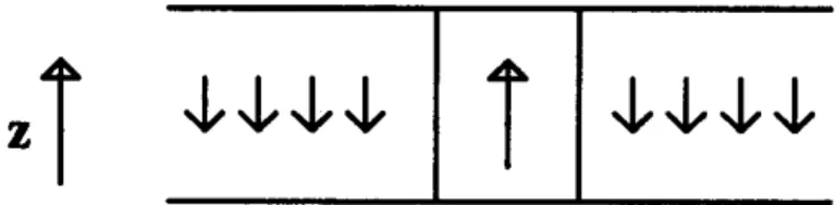
Wecanuse thesesimpleconceptstoobtainanestimateforthe horizontal
areaoccupiedbyprecipitatingdisturbances(seeFig. 2.3). Simplyfrommass
conservation, the ratio of the area of ascent to descent must be inversely
proportional to the ratio of the corresponding vertical velocities. Using the
guresgivenabove,thisratiois1/3,butallowingforasmallerNinconvective
regions willdecrease this somewhat, closer toGray`s estimateof 1/5.
Figure 2.4: Schematic diagram showing relatively strong updraughts occu-
pying a much smaller horizontal area than the much weaker compensating
downdraughts.
2.5 Some further notes on the scaling at low
latitudes
1. In mid-latitudes R o << 1 and it is a convenient small parameter for
asymptotic expansion. However, generally at low latitudes as f ! 0,
R o 1 and we must seek other parameters. One such parameter,
(R iR o) 1
is always small, even if L10 7
m.
2. The vorticity equation contains useful information. It tells us that
synoptic-scale phenomena (L 10 6
m) are nearly uncoupled in the
vertical except incircumstances that limit(2.29). These are:
a. Q=c
p
large. Then w is scaled from the thermodynamic equation
suchthat wN 2
=gQ=(c
p T).
b. For planetary-scale motions (L 10 7
) of the type discussed in
Chapter1,wehaveagainR o<<1. Then,ifDH
p
asbefore,the
quasi-geostrophicscaling(e.g.,2.24)appliesoncemore. Moreover,
the appropriate vorticity equation is (2.28) instead of (2.29). In
this case, couplingin the vertical isre-established.
c. If the motions involve vertically-propagating gravity waves with
D << H
p
, but still with L 10 7
m and if U ! 0, then again
R o<<1 and verticalcoupling occurs.
As a consequence of (2.29), the atmosphere is governed by barotropic
processes. Thatis,theusualbaroclinicwayofproducingkineticenergyfrom
potential energy, i.e., the lifting of warm air and the lowering of cold air,
does not occur. It follows then that energy transfers are strictly limited.
Howthen can the kinetic energy be generatedin the tropics? Obviously the
answer lies in convective processes. But if this is so, why are the thermal
elds so at? This will be addressed later. However it is interesting at this
pointto gain some insight intothis feature of the tropicalatmosphere.
If wN 2
=g Q=(c
p
T), then < w 0
T 0
> g < Q 0
T 0
> =(N 2
c
p
T). Now
<w 0
T 0
>measurestherateofproductionofkineticenergyandg <Q 0
T 0
>is
proportionaltotherateofproductionofpotentialenergy(i.e. heatingwhere
it is hot and cooling where it is cold). Thus the statement < w 0
T 0
>g <
Q 0
T 0
>=(N 2
c
p
T) implies that, in the tropics, potential energy is converted
tokineticenergyassoonasitisgenerated. Inotherwordsthereisnostorage
ofpotentialenergy. WeknowfromscalingprinciplesthatwN 2
=g Q=(c
p T),
as@=@t andVr arerelativelysmallinthetropics(seesection2.3). Since
large precipitation implies large Q, itfollows that w must be comparatively
IfrT werelarge,athirdtermwouldentersuchthat<w 0
T 0
>+(g=N 2
)<
T 0
V 0
> rT < Q 0
T 0
> =(c
p
T) and this is tantamount to having storage
even if V is the same inboth cases.
2.6 The weak temperature gradient approxi-
mation
Onecanderiveabalancedtheoryformotionsinthedeeptropicsbyassuming
that @=@t and Vr are much less than w(@=@z),whereupon
w
@
@z
= D
Dt
=S
; (2.31)
where S
=Q=(c
p
), =(p=p
o )
is the Exner function, and p
o
=1000 mb.
The vorticity equation(2.28) may be written
@
@t
+V r
(+f)=(+f)D (2.32)
whereDisthe horizontaldivergencerV,andthecontinuityequationgives
D=rV= 1
@(w)
@z
: (2.33)
Using(2.31) the vorticity equation becomes
@
@t
+Vr
(+f)=
(+f)
@
@z
S
@=@z
: (2.34)
Iftherewerenodiabaticheating(S
=0),theright-hand-sideof(2.33)would
be zero and absolute vorticity values would be simply advected around at
xed elevation by the horizontal wind. The role of heating is to produce
vertical divergence, which, in turn, decreases the absolute vorticity if the
divergenceispositiveandincreasesitifthedivergenceisnegative(i.e. ifthere
is horizontal convergence). If the divergence and the horizontal wind elds
are known, it is therefore possible to predict the evolution of the absolute
vorticity eld.
Thenal diÆcultyispredicting thehorizontalwindeld. The horizontal
windcomponentscanbewrittenassumsofpartsderived fromastreamfunc-
tion and parts derived froma velocity potential:
v
x
=
@
@y +
@
@x v
y
=
@
@x +
@
@y
: (2.35)
However, and may be writtenin terms of
a
and D:
r 2
=
a
f (2.36)
r 2
=D (2.37)
where r 2
is the horizontal Laplacianoperator. Equations (2.36) and (2.37)
arereadilysolvedfor andusingstandardnumericalmethods, afterwhich
the horizontalvelocitymay bedeterminedfrom(2.35). Given the horizontal
velocity and the divergence, we have the tools needed to completely solve
the vorticity equation. In practice, (2.34), stepped forward in time and the
diagnostic equations (2.36) and (2.37) are solved after each time step to
enable the velocity eld to be updated using (2.35). All that is required to
close the system is amethodof specifying the heatingterm S
.
The principal determinant of the sign of the horizontal divergence in
(2.33) is the sign of @S
=@z. If heating increases with height, divergence is
negative, and the magnitude of the absolute vorticity increases with time,
whereas S
decreasingwithheightresultsinpositivedivergenceand decreas-
ingabsolutevorticity. Deepconvectiongenerallyresultsinincreasingvortic-
ityorspinupinthelowertroposphereandspindownintheuppertroposphere,
whereas other regions typically dominated by radiative cooling and shallow
convection tend toexperience the reverse.
In spite of the fact that tropical storms don't formally obey the weak
temperature gradient approximation, the above picture holds qualitatively
for them as well. However, gravity wave dynamics are not encompassed by
this picture, so the wind perturbations associated with these waves are not
captured. Furthermore, consideration of frictional eects is important to
the quantitative prediction of tropical ows, especially in the long term. In
spite of these deciencies, the above picture of tropical dynamics should be
useful for understanding the short-term evolution of most tropical weather
systems. In a later chapter we approach the problem of determining the
pattern of heating associated with moist convection. More details on the
weak temperature gradient approximation can be found in papers by Sobel
and Bretherton (2000), Sobel et al. (2001) and Raymond and Sobel (2001).