The Tragedy of Annuitization

IHS Economics Series Working Paper 268

May 2011

The Tragedy of Annuitization

Ben J. Heijdra

Jochen O. Mierau

Laurie S.M. Reijnders

Impressum Author(s):

Ben J. Heijdra, Jochen O. Mierau, Laurie S.M. Reijnders Title:

The Tragedy of Annuitization ISSN: Unspecified

2011 Institut für Höhere Studien - Institute for Advanced Studies (IHS) Josefstädter Straße 39, A-1080 Wien

E-Mail: o ce@ihs.ac.atffi Web: ww w .ihs.ac. a t

All IHS Working Papers are available online: http://irihs. ihs. ac.at/view/ihs_series/

This paper is available for download without charge at:

https://irihs.ihs.ac.at/id/eprint/2059/

The Tragedy of Annuitization

Ben J. Heijdra, Jochen O. Mierau, Laurie S. M. Reijnders

268

Reihe Ökonomie

Economics Series

268 Reihe Ökonomie Economics Series

The Tragedy of Annuitization

Ben J. Heijdra, Jochen O. Mierau, Laurie S. M. Reijnders May 2011

Contact:

Ben J. Heijdra

Faculty of Economics and Business University of Groningen

P.O. Box 800

9700 AV Groningen, The Netherlands

: +31/50/363-7303 Fax: +31/50/363-7337 email: info@heijdra.org and

Institute for Advanced Studies, CESifo, Netspar Jochen O. Mierau

Faculty of Economics and Business University of Groningen

P.O. Box 800

9700 AV Groningen, The Netherlands

: +31/50/363-8534 Fax: +31/50/363-7337 email: j.o.mierau@rug.nl Laurie S.M. Reijnders

Faculty of Economics and Business University of Groningen

P.O. Box 800

9700 AV Groningen, The Netherlands

: +31/50/363-4001 Fax: +31/50/363-7337 email: lauriereijnders@gmail.co

Founded in 1963 by two prominent Austrians living in exile – the sociologist Paul F. Lazarsfeld and the economist Oskar Morgenstern – with the financial support from the Ford Foundation, the Austrian Federal Ministry of Education and the City of Vienna, the Institute for Advanced Studies (IHS) is the first institution for postgraduate education and research in economics and the social sciences in Austria. The Economics Series presents research done at the Department of Economics and Finance and aims to share “work in progress” in a timely way before formal publication. As usual, authors bear full responsibility for the content of their contributions.

Das Institut für Höhere Studien (IHS) wurde im Jahr 1963 von zwei prominenten Exilösterreichern – dem Soziologen Paul F. Lazarsfeld und dem Ökonomen Oskar Morgenstern – mit Hilfe der Ford- Stiftung, des Österreichischen Bundesministeriums für Unterricht und der Stadt Wien gegründet und ist somit die erste nachuniversitäre Lehr- und Forschungsstätte für die Sozial- und Wirtschafts- wissenschaften in Österreich. Die Reihe Ökonomie bietet Einblick in die Forschungsarbeit der Abteilung für Ökonomie und Finanzwirtschaft und verfolgt das Ziel, abteilungsinterne Diskussionsbeiträge einer breiteren fachinternen Öffentlichkeit zugänglich zu machen. Die inhaltliche Verantwortung für die veröffentlichten Beiträge liegt bei den Autoren und Autorinnen.

Abstract

We construct a tractable discrete-time overlapping generations model of a closed economy and use it to study government redistribution of accidental bequests and private annuities in general equilibrium. Individuals face longevity risk as there is a positive probability of passing away before the retirement period. We find non-pathological cases where it is better for long- run welfare to waste accidental bequests than to give them to the elderly. Next we study the introduction of a perfectly competitive life insurance market offering actuarially fair annuities.

There exists a tragedy of annuitization: although full annuitization of assets is privately optimal it is not socially beneficial due to adverse general equilibrium repercussions.

Keywords

Longevity risk, risk sharing, overlapping generations, intergenerational transfers, annuity markets

JEL Classification

D52, D91, E10, J20

Contents

1 Introduction 1

2 The model 3

2.1 Consumers ... 3

2.2 Demography ... 5

2.3 Production ... 5

2.4 Government ... 6

2.5 Equilibrium ... 7

3 The exogenous growth model 8

3.1.1 Transfers to the old ... 14

3.1.2 Transfers to the young ... 18

3.2 Welfare analysis ... 20

3.2.1 Transfers to the old ... 21

3.2.2 Transfers to the young ... 26

4 Tragedy of annuitization 27

4.2 From transfers to the young to perfect annuities ... 31

4.3 Discussion ... 37

5 The endogenous growth model 38

6 Conclusion 42

References 44

1 Introduction

Although death is one of the true certainties in life, the date at which it occurs is unknown to all but the most desperate individuals. Faced with life-time uncertainty, rational non-altruistic agents must balance the risk of leaving unconsumed wealth in the form of unintended (acci- dental) bequests against the risk of running out of resources in old age. As was shown in the classic analysis of Yaari (1965) and more recently by Davidoff et al. (2005), life annuities are very attractive insurance instruments in the presence of longevity risk. Intuitively, annuities allow for risk sharing between lucky (long-lived) and unlucky (short-lived) individuals (Kot- likoff et al., 1986). These increased risk-sharing opportunities ensure that life annuities are welfare maximizing from a microeconomic perspective, i.e. in a partial equilibrium setting.

From a macroeconomic perspective, however, it is not immediately clear whether or not annuities are welfare improving. There are two key mechanisms that are ignored in a partial equilibrium analysis. First, in the absence of private annuities there will be accidental bequests which, provided they are redistributed in one way or another to surviving agents, boost the consumption opportunities of such agents. See, among others, Sheshinski and Weiss (1981), Abel (1985), Pecchenino and Pollard (1997), and Fehr and Habermann (2008) on this point.

Second, the availability of annuities affects the rate of return on an individual’s savings. As a result, aggregate capital accumulation will generally depend on whether or not annuity opportunities are available. Capital accumulation in turn determines wages and the interest rate if factor prices are endogenous.

The objective of this paper is to study the general equilibrium effects of life annuities.

Our model has the following features. First, we postulate a simple general equilibrium model of a closed economy. On the production side we allow for a capital accumulation externality of the form proposed by Romer (1989). The production model is quite flexible in that it can accommodate both the exogenous and the endogenous growth models as special cases.

Second, we assume that the economy is populated by overlapping generations of two- period-lived agents facing longevity risk. Just as in the Diamond (1965) model life consists of two phases, namely youth and old age, but unlike that model there is a positive probability of death at the end of youth. At birth, agents are identical in the sense that they feature the same preferences, have the same labour productivity, and face the same death probability.

the government. We investigate the general equilibrium effects of three prototypical revenue recycling schemes. In particular, the policy maker can (a) engage in wasteful expenditure (the WE scenario), (b) give lump-sum transfers to the old (the TO scenario), or (c) provide lump-sum transfers to the young (the TY scenario).

Fourth, we compare the different revenue recycling schemes with the case in which an- nuities are available. In particular, we assume that private annuity markets are perfectly competitive. With perfect annuities (the PA scenario) the probability of death determines the wedge between the rate of return on physical capital and the annuity rate of return. Since the latter exceeds the former, rational non-altruistic individuals fully annuitize their savings.

The main finding of the paper concerns the phenomenon which we call the tragedy of annuitization: although full annuitization of assets is privately optimal it may not be socially beneficial due to adverse general equilibrium repercussions. If all agents invest their financial wealth in the annuity market then the resulting long-run equilibrium leaves everyone worse off compared to the case where annuities are absent and accidental bequests are redistributed to the young (or even wasted by the government). In the exogenous growth model we demon- strate the existence of two versions of the tragedy. In thestrong version, opening up perfect annuity markets in an economy in which accidental bequests initially go to waste (switch from WE to PA) results in a decrease in steady-state welfare of newborns. Interestingly, this rather surprising result holds for a reasonable (i.e., low) value of the intertemporal substitu- tion elasticity. In such a case the beneficial effects of annuitization are more than offset by a substantial drop in the long-run capital intensity and in wages. Future newborns would have been better off if no annuity markets had been opened.

There is also aweak version of the tragedy in the exogenous growth model. If the economy is initially in the equilibrium with accidental bequests flowing to the young, then opening up annuity markets will reduce steady-state welfare regardless of the magnitude of the intertem- poral substitution elasticity. Intuitively, private annuities redistribute assets from deceased to surviving elderly in an actuarially fair way whereas transferring unintended bequests to the young constitutes an intergenerational transfer. This intergenerational transfer induces beneficial savings effects, which, in the end, lead to higher welfare.

In the endogenous growth model and restricting attention to realistic values for the in- tertemporal substitution elasticity, both versions of the tragedy show up in terms of the

macroeconomic growth rate. Growth is highest in the TY case, and the rate under the WE case exceeds the one for the PA scenario.

The structure of the paper is as follows. Section 2 presents the model in its most general form. Section 3 studies the analytical properties of the exogenous growth version of the model.

It also computes, both analytically and quantitatively, the allocation and welfare effects of scenario switches. Section 4 is the core of the paper. It shows what happens to allocation and welfare if a perfectly competitive annuity market is opened up at some point in time. It also highlights the importance of initial conditions, i.e. it demonstrates that the results depend not only on the availability of annuities but also on the scenario that is replaced by these insurance markets. Section 5 briefly discusses the effects of annuitization in the endogenous growth version of the model. Section 6 restates the main results and presents some possible extensions. All mathematical details can be found in Heijdra, Mierau, and Reijnders (2010).

2 The model

2.1 Consumers

Each agent lives for a maximum of two periods and faces a positive probability of death between the first and the second period. Agents work full-time during the first period of their lives (termed “youth”) and – if they survive – retire in the second period (“old age”). The expected lifetime utility of an individual born at timetis given by:

EΛ^y_t ≡U(C_t^y) +1−π

1 +ρU(C_t^o+1), (1)

whereC_t^y andC_t^o+1are consumption during youth and old age, respectively, ρ >0 is the pure rate of time preference, and π > 0 is the probability of death. Individuals have no bequest motive and, therefore, attach no utility to savings that remain after they die. We assume that the utility function is of the CRRA type:

U(C) =









C^1−1/σ−1

1−1/σ ifσ >0, σ6= 1,

lnC ifσ = 1,

(2)

whereσis the elasticity of intertemporal substitution. The agent’s budget identities for youth and old age are given by:

C_t^y+S_t=w_t+Z_t^y, (3a)

C_t^o+1 =Z_t^o+1+ (1 +r_t+1)S_t, (3b)

wherew_tis the wage rate, r_t is the interest rate,S_t denotes the level of savings, andZ_t^y and Z_t^o₊₁ are transfers received from the government during either youth or old age (see below).

Combining the equations in (3) yields the consolidated lifetime budget constraint:

C_t^y+ C_t^o₊₁ 1 +r_t+1

=w_t+Z_t^y+ Z_t^o₊₁ 1 +r_t+1

. (4)

If an agent dies before reaching old age his savings flow to the government in the form of an accidental bequest. Due to mortality risk agents are not allowed to hold negative savings (i.e.

loans). In case of premature death their loans would be unaccounted for.

The agent chooses C_t^y, C_t^o₊₁ and S_t in order to maximize expected lifetime utility (1) subject to the budget constraint (4) and a non-negativity constraint on savings. Assuming an interior optimum (S_t>0), the agent’s optimal plans are fully characterized by:

C_t^y = Φ (r_t+1)

w_t+Z_t^y+ Z_t^o₊₁ 1 +rt+1

, (5)

C_t^o+1

1 +r_t+1

= [1−Φ (rt+1)]

wt+Z_t^y+ Z_t^o+1

1 +r_t+1

, (6)

S_t= [1−Φ (r_t+1)] [w_t+Z_t^y]−Φ (r_t+1) Z_t^o₊₁ 1 +rt+1

, (7)

where Φ(r_t+1) is the marginal propensity to consume out of total wealth (wage income and transfers) in the first period:

Φ (r_t+1)≡

1 +

1−π 1 +ρ

σ

(1 +r_t+1)^σ−1 −1

, 0<Φ (·)<1. (8)

Note that the impact of a change in the future interest rate on current savings is fully de- termined by the elasticity of intertemporal substitution σ. For the special case with σ = 1 (logarithmic utility) savings are completely independent of the interest rate.¹ The income

1If the government provides transfers to the old (Zt+1^o >0) there is also a positive human wealth effect on saving. In this paper, however, such transfers are proportional to the interest factor, 1 +rt+1, so that this human wealth effect is not operative. If the agent would also work in old age then the human wealth effects would result in an increase in the savings elasticity.

effect of a higher interest rate is exactly offset by the substitution effect induced by a lower price of second period consumption. In the more general case with σ > 1 savings increase as the interest increases because the substitution effect dominates the income effect. If, on the other hand, σ <1 the income effect is stronger than the substitution effect and savings decline as the interest rate rises.²

2.2 Demography

The population grows at an exogenous rate n > 0 so that every period a cohort of Lt = (1 +n)L_t−1 young agents is born. In principle each generation lives for two periods, but not all of its members survive the transition from youth to old age. The total population at time tis equal to P_t≡(1−π)L_t−1+L_t.

2.3 Production

There is a constant and large number of identical and perfectly competitive firms. The technology available to each individual firmiis given by:

Y_it= Ω_tK_it^αN_it^1−α, 0< α <1, (9)

where Y_it is output, K_it is the employed capital stock, N_it is the amount of labour used in the production process, α is the capital share of output and Ω_t is the aggregate level of technology in the economy which is considered as given by individual firms. Factor demands of the individual firm are given by the following marginal productivity conditions:

w_t= (1−α) Ω_tk^α_it, (10a)

r_t+δ =αΩ_tk_it^α−1, (10b)

wherek_it≡K_it/N_itis the capital intensity of firmiandδ >0 is the depreciation rate. Under the assumption of perfect competition in both factor markets all firms face the same factor prices and, therefore, they all choose the same level of capital intensity k_it=k_t.

2From the empirical perspective the most relevant case appears to be the one with 0 < σ <1. See, for example, Skinner (1985) and Attanasio and Weber (1995) who report estimates ranging between, respectively, 0.3 to 0.5, and 0.6 to 0.7.

Generalizing the insights of Pecchenino and Pollard (1997, p. 28) to a growing population we postulate that the inter-firm investment externality takes the following form:

Ω_t= Ω0k^η_t, 0< η≤1−α, (11)

where Ω0 is a constant, k_t≡K_t/N_t is the economy-wide capital intensity,K_t≡P

iK_it is the total stock of capital and N_t≡P

iN_it is the total labour force.

According to (11) total factor productivity increases in line with the aggregate capital intensity in the economy. That is, if an individual firm increases its capital stock all firms benefit through a boost in the general productivity level Ω_t. The strength of this inter-firm investment externality is governed by the parameter η. If 0 ≤ η <1−α then the long-run growth rate in per capita variables is exogenously determined and equal to zero. In the knife- edge case with η = 1−α the investment externality exactly offsets the decrease in marginal productivity following an addition to the capital stock. The aggregate production sector then exhibits single-sector endogenous growth of the type described in Romer (1989).

Using the general productivity index (11) we can write output (9) and factor prices (10) in aggregate terms:

y_t= Ω0k^α_t^+η, (12)

w_t= (1−α) Ω0k^α_t^+η, (13)

r_t=αΩ0k_t^α+η−1−δ, (14)

wherey_t≡Y_t/N_t is the level of output per worker and Y_t≡P

iY_it is aggregate output. We assume that the economy is sufficiently productive to assure a positive interest rate even when the investment externality attains its knife-edge value, i.e. αΩ0 > δ.

2.4 Government

The government administers the allocation of the accidental bequests, maintains a period-by- period balanced budget, and does not issue debt or retain funds. The government’s budget constraint is therefore given by:

π(1 +r_t)L_t−1S_t−1= (1−π)L_t−1Z_t^o+L_tZ_t^y+G_t. (15) That is, the total assets left behind by the agents who perish before reaching old age (left-hand side) are used to finance total transfers to the survivors Z_t^o, transfers to the newly arrived

youngZ_t^y, and unproductive government expenditure G_t.

We assume that the government can choose between two financing scenarios. Either it redistributes all its proceeds among the surviving agents in the form of lump-sum transfers or it uses the funds solely for unproductive government spending.

Transfer scenario. The government can either give the revenues exclusively to the young or exclusively to the old.³

(TY) If all the proceeds go to the young thenZ_t^o =G_t= 0 in (15) and transfers to the young are given by:

Z_t^y = π(1 +rt)Lt−1St−1

L_t . (16a)

(TO) If all the transfers accrue to the elderly, both Z_t^y =G_t= 0 in (15) and transfers to the old are given by:

Z_t^o= π(1 +rt)Lt−1St−1

(1−π)L_t−1 . (16b)

Unproductive spending scenario.

(WE) If the full receipts from accidental bequests are used for unproductive government spend- ing then Z_t^y =Z_t^o= 0 in (15) and wasteful government expenditures are:

G_t=π(1 +r_t)L_t−1S_t−1. (16c)

2.5 Equilibrium

In equilibrium both factor markets must clear. As all young agents work full-time and all old agents are retired, the labour market equilibrium condition simply states that the total labour force must equal the total number of young agents, i.e. Nt=Lt. The capital market clearing condition implies that aggregate savings of the generation born at timet−1 must be equal to the total stock of productive capital in period t, i.e. Kt =Lt−1St−1. It immediately follows

3Any convex combination of these two options is also feasible. We focus on the two extreme cases for ease of illustration.

that, in equilibrium, the three revenue recycling scenarios implied by (16a)-(16c) above can be rewritten as:

Z_t^y =π(1 +r_t)k_t, (17a)

Z_t^o = 1 +n

1−ππ(1 +r_t)k_t, (17b)

g_t=π(1 +r_t)k_t, (17c)

where g_t≡G_t/L_t are per worker government expenditures.

Substituting per capita savings (7) into the capital market clearing condition and using the aggregate factor prices (13) and (14) provides the fundamental difference equation of the model:

(1 +n)kt+1= [1−Φ (rt+1)] [wt+Z_t^y]−Φ (rt+1) Z_t^o+1

1 +r_t+1

. (18)

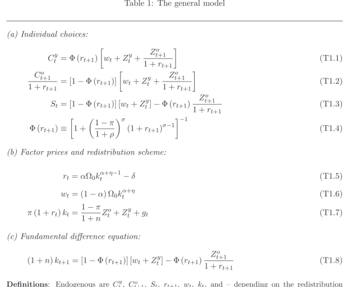
For future reference we summarize the system of equations that characterizes the macro- economic equilibrium in Table 1. Equations (T1.1)–(T1.3) are the consumption and saving demand functions, (T1.4) states the definition for the marginal propensity to consume, equa- tions (T1.5) and (T1.6) are the factor prices, (T1.7) is the government budget constraint with capital market equilibrium imposed, and (T1.8) is the fundamental difference equation.

3 The exogenous growth model

In this section and the next we study the exogenous growth version of our model, i.e. we assume that the capital accumulation externality parameter satisfies 0 ≤η < 1−α so that there are diminishing returns to the macroeconomic capital stock. (The knife-edge model with η = 1−α is briefly discussed in Section 5 below.) Throughout the paper we assume that the steady-state interest rate exceeds the rate of population growth. Empirical support for this assumption is provided by Abel et al. (1987).

Assumption 1 [Dynamic efficiency] For each scenario the corresponding steady-state inter- est raterˆsatisfiesr > n.ˆ

3.1 Stability and transition

We first study the dynamic properties of the model under the assumption that the government wastes the revenues from accidental bequests (the WE scenario). One of the crucial structural

Table 1: The general model

(a) Individual choices:

C_t^y = Φ (rt+1)

wt+Z_t^y+ Z_t^o+1

1 +r_t+1

(T1.1) C_t^o+1

1 +r_t+1

= [1−Φ (r_t+1)]

w_t+Z_t^y+ Z_t^o+1

1 +r_t+1

(T1.2) St= [1−Φ (rt+1)] [wt+Z_t^y]−Φ (rt+1) Z_t^o+1

1 +r_t+1

(T1.3) Φ (rt+1)≡

1 +

1−π 1 +ρ

σ

(1 +rt+1)^σ−1 −1

(T1.4) (b) Factor prices and redistribution scheme:

r_t=αΩ0k_t^α+η−1−δ (T1.5)

w_t= (1−α) Ω0k^α_t^+η (T1.6)

π(1 +r_t)k_t= 1−π

1 +nZ_t^o+Z_t^y+g_t (T1.7)

(c) Fundamental difference equation:

(1 +n)k_t+1= [1−Φ (r_t+1)] [w_t+Z_t^y]−Φ (r_t+1) Z_t^o₊₁ 1 +r_t+1

(T1.8) Definitions: Endogenous are C_t^y, C_t+1^o , St, rt+1, wt, kt, and – depending on the redistribution scheme – one ofZ_t^y orZ_t^oorgt. Parameters: mortality rateπ, population growth raten, rate of time preference ρ, capital coefficient in the technologyα, investment externality coefficient η, scale factor in the technology Ω0, and depreciation rate of capitalδ.

parameters is the intertemporal substitution elasticity,σ. Whilst the model can accommodate a wide range of values forσ, we nevertheless make the following assumption.

Assumption 2 [Admissible values for σ] The intertemporal substitution elasticity satisfies:

0< σ≤σ¯ ≡ 2−α−η 1−α−η.

We defend this assumption on two grounds. First, the restriction is very mild. Indeed, empirical evidence suggests that σ falls well short of unity whereas – even in the absence of external effects (η = 0) – ¯σ is much larger than unity. For example, for a capital share of α = 0.3 we find that ¯σ = 2.43. In the presence of external effects (η > 0) ¯σ is even larger.

Second, by restricting the range of admissible values forσ the existence and stability proofs are simplified substantially.

The fundamental difference equation under the WE scenario can be written as follows:

[Ψ (k_t+1)≡] k_t+1

1−Φ (k_t+1) = (1−α) Ω0

1 +n k_t^α+η [≡Γ (k_t)], (19)

where Φ (k) is given by:⁴ Φ (k)≡

1 +

1−π 1 +ρ

σ

1−δ+αΩ0k^α+η−1σ−1−1

. (20)

It is easy to show that Ψ^′ >0 and Γ^′ >0. We can prove the following proposition.

Proposition 1 [Existence and stability of the WE model] Consider the WE model as given in (19)–(20) and adopt Assumption 2. The following properties can be established:

(i) The model has two steady-state solutions; the trivial one features k_t+1 = k_t = 0, and the economically relevant satisfies k_t+1=k_t= ˆk^WE, where ˆk^WE is the solution to:

kˆ^WE

1−Φ(ˆk^WE) = (1−α) Ω0

1 +n (ˆk^WE)^α+η.

(ii) The trivial steady-state solution is unstable whilst the non-trivial solution is stable:

0< dk_t+1

dkt

<1, for k_t+1 =k_t= ˆk^WE.

For any positive initial value the capital intensity converges monotonically to kˆ^WE.

4Equation (20) is obtained by substituting (T1.5) into (8).

Proof: See Heijdra et al. (2010, Appendix A).

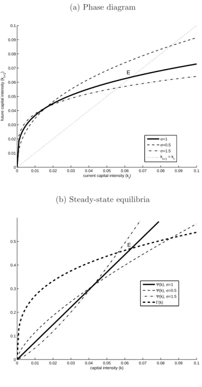
We visualize the corresponding phase diagram in Figure 1(a) for different values of the intertemporal substitution elasticity. This figure is based on the following plausible parameter values that are used throughout much of the paper. In the benchmark case we assume that the elasticity of intertemporal substitution is σ= 1 (i.e. log-utility), and that the investment externality is absent (η = 0). Each phase of life covers 40 years, the population grows by one percent per annum (so that n= (1 + 0.01)⁴⁰−1 = 0.49), individuals face a probability of death between youth and old age of thirty percent (π = 0.3), the capital share of output is thirty percent (α = 0.3), and the depreciation rate of capital is six percent per annum (δ = 0.92). We set the production function constant and time preference rate such that output per worker is equal to unity and the interest rate is four percent per annum (ˆr= 3.80) in the WE scenario. We obtain Ω0 = 2.29 and ρ = 3.47 or 3.82% annually. The resulting steady-state values of the key variables of the model are given in Table 2(a).⁵ Note that Assumptions 1 and 2 are both satisfied for this calibration.

In Figure 1(a) the solid line represents the fundamental difference equation (19) (for σ = 1) and the dotted line is the steady-state conditionkt+1 =kt.⁶ The economically relevant steady-state equilibrium is at point E where the slope of (19) is strictly less than unity. Figure 1(b) plots Ψ (k) (for different values ofσ) and Γ (k) separately. It conveniently illustrates the existence and stability properties of the two steady-state equilibria. In particular, it visualizes Proposition 1(ii) which proves that Γ(k) is steeper (flatter) than Ψ(k) around k= 0 (k= ˆk) for all feasible values ofσ.

Suppose that at some time t the economy has converged to the steady-state implied by the WE scenario, i.e. k_t= ˆk^WE. What would happen at impact, during transition, and in the long run if the government were to switch to a transfer scenario? We study two such policy switches in turn, namely from WE to TO and from WE to TY.

5For different values ofσwe re-calibrate the model (by choice ofρand Ω0) such that output and the interest rate remain the same in the WE scenario.

6The dash-dotted and dashed lines in Figure 1(a) represent the fundamental difference equation for different values of the intertemporal substitution elasticity, σ. Mathematically, these lines are described by k =

Figure 1: Phase diagram and steady-state equilibria (a) Phase diagram

0 0.01 0.02 0.03 0.04 0.05 0.06 0.07 0.08 0.09 0.1

0 0.01 0.02 0.03 0.04 0.05 0.06 0.07 0.08 0.09 0.1

E

current capital intensity (k t) future capital intensity (kt+1)

σ=1 σ=0.5 σ=1.5 kt+1 = k

t

(b) Steady-state equilibria

0 0.01 0.02 0.03 0.04 0.05 0.06 0.07 0.08 0.09 0.1

0 0.1 0.2 0.3 0.4

0.5 E

capital intensity (k)

Ψ(k), σ=1 Ψ(k), σ=0.5 Ψ(k), σ=1.5 Γ(k)

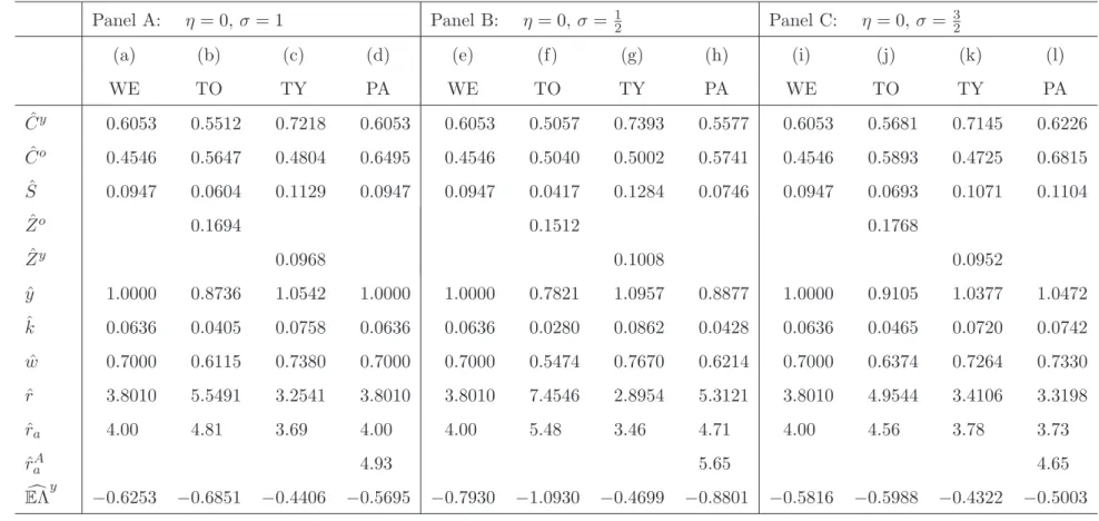
Table 2: Steady-state values with exogenous growth^⋆

Panel A: η= 0,σ = 1 Panel B: η = 0,σ = ¹₂ Panel C: η= 0, σ= ³₂

(a) (b) (c) (d) (e) (f) (g) (h) (i) (j) (k) (l)

WE TO TY PA WE TO TY PA WE TO TY PA

Cˆ^y 0.6053 0.5512 0.7218 0.6053 0.6053 0.5057 0.7393 0.5577 0.6053 0.5681 0.7145 0.6226 Cˆ^o 0.4546 0.5647 0.4804 0.6495 0.4546 0.5040 0.5002 0.5741 0.4546 0.5893 0.4725 0.6815 Sˆ 0.0947 0.0604 0.1129 0.0947 0.0947 0.0417 0.1284 0.0746 0.0947 0.0693 0.1071 0.1104

Zˆ^o 0.1694 0.1512 0.1768

Zˆ^y 0.0968 0.1008 0.0952

ˆ

y 1.0000 0.8736 1.0542 1.0000 1.0000 0.7821 1.0957 0.8877 1.0000 0.9105 1.0377 1.0472 kˆ 0.0636 0.0405 0.0758 0.0636 0.0636 0.0280 0.0862 0.0428 0.0636 0.0465 0.0720 0.0742

ˆ

w 0.7000 0.6115 0.7380 0.7000 0.7000 0.5474 0.7670 0.6214 0.7000 0.6374 0.7264 0.7330 ˆ

r 3.8010 5.5491 3.2541 3.8010 3.8010 7.4546 2.8954 5.3121 3.8010 4.9544 3.4106 3.3198 ˆ

r_a 4.00 4.81 3.69 4.00 4.00 5.48 3.46 4.71 4.00 4.56 3.78 3.73

ˆ

r^A_a 4.93 5.65 4.65

EcΛ^y −0.6253 −0.6851 −0.4406 −0.5695 −0.7930 −1.0930 −0.4699 −0.8801 −0.5816 −0.5988 −0.4322 −0.5003

13

3.1.1 Transfers to the old

The effects of a policy switch from the WE scenario to the TO scenario can be studied with the aid of the following fundamental difference equation:

[Ψ (k_t+1, z1)≡] 1 +z1 π

1−πΦ (kt+1)

1−Φ (k_t+1) k_t+1= Γ (k_t), (21)

where Γ (k_t) is defined in (19) above, z1 is a perturbation parameter (0 ≤ z1 ≤ 1) and Ψ (k_t+1, z1) features positive partial derivatives Ψ_k>0 and Ψ_z1 >0. The case withz1= 0 is the WE scenario whilst for z1 = 1 the TO case is obtained. The policy switch thus consists of a unit increase in z1 occurring at time t in combination with the initial conditionk_t= ˆk^WE. We provide the following proposition.

Proposition 2 [Existence and stability of the TO model] Consider the TO model as given in (21) and adopt Assumption 2. The following properties can be established:

(i) The model has two steady-state solutions; the trivial one features k_t+1 = k_t = 0, and the economically relevant one satisfies kt+1=kt= ˆk^TO, where ˆk^TO is the solution to:

1 +_1−π^π Φ(ˆk^TO) 1−Φ(ˆk^TO)

kˆ^TO = (1−α) Ω0

1 +n (ˆk^TO)^α+η.

(ii) The trivial steady-state solution is unstable whilst the non-trivial solution is stable:

0< dkt+1

dk_t <1, for k_t+1 =k_t= ˆk^TO.

For any positive initial value the capital intensity converges monotonically to kˆ^TO. (iii) The steady-state capital intensity satisfies the following inequality:

0<kˆ^TO <ˆk^WE.

Proof: See Heijdra et al. (2010, Appendix B).

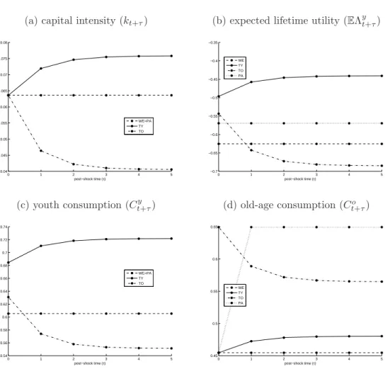
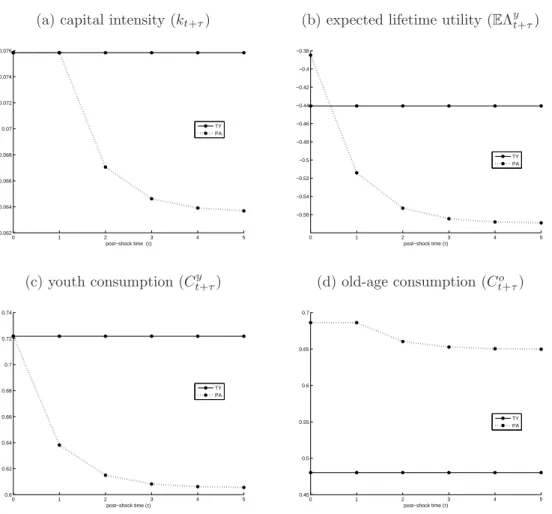
For σ = 1 we visualize the transitional dynamics of the capital intensity in Figure 2(a) whilst the quantitative long-run results are reported in Table 2(b). In Figure 2(a) the hor- izontal axis records post-shock time τ and the vertical axis gives the values of kt+τ. By giving transfers to old agents, the old at the time of the policy switch (τ = 0) are able to

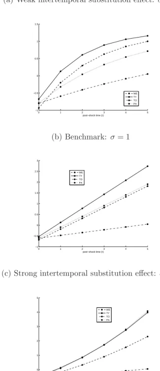
Figure 2: Transitional dynamics in the exogenous growth model Panel A: Benchmark: σ = 1

(a) capital intensity (kt+τ) (b) expected lifetime utility (EΛ^y_t+τ)

0 1 2 3 4 5

0.04 0.045 0.05 0.055 0.06 0.065 0.07 0.075 0.08

post−shock time (τ)

WE=PA TY TO

0 1 2 3 4 5

−0.7

−0.65

−0.6

−0.55

−0.5

−0.45

−0.4

−0.35

post−shock time (τ) WE

TY TO PA

(c) youth consumption (C_t+τ^y ) (d) old-age consumption (C_t+τ^o )

0 1 2 3 4 5

0.54 0.56 0.58 0.6 0.62 0.64 0.66 0.68 0.7 0.72 0.74

post−shock time (τ)

WE=PA TY TO

0 1 2 3 4 5

0.45 0.5 0.55 0.6 0.65

post−shock time (τ) WE

TY TO PA

(Figure 2, continued)

Panel B: Weak intertemporal substitution effect: σ = ¹₂

(e) capital intensity (kt+τ) (f) expected lifetime utility (EΛ^y_t+τ)

0 1 2 3 4 5

0.02 0.03 0.04 0.05 0.06 0.07 0.08 0.09

post−shock time (τ) WE

TY TO PA

0 1 2 3 4 5

−1.1

−1

−0.9

−0.8

−0.7

−0.6

−0.5

−0.4

post−shock time (τ) WE

TY TO PA

(g) youth consumption (C_t^y+τ) (h) old-age consumption (C_t^o+τ)

0 1 2 3 4 5

0.5 0.55 0.6 0.65 0.7 0.75

post−shock time (τ) WE

TY TO PA

0 1 2 3 4 5

0.45 0.5 0.55 0.6 0.65

post−shock time (τ)

WE TY TO PA

(Figure 2, continued)

Panel C: Strong intertemporal substitution effect: σ = ³₂

(i) capital intensity (kt+τ) (j) expected lifetime utility (EΛ^y_t+τ)

0 1 2 3 4 5

0.045 0.05 0.055 0.06 0.065 0.07 0.075

post−shock time (τ) WE

TY TO PA

0 1 2 3 4 5

−0.6

−0.58

−0.56

−0.54

−0.52

−0.5

−0.48

−0.46

−0.44

−0.42

post−shock time (τ)

WE TY TO PA

(k) youth consumption (C_t^y+τ) (l) old-age consumption (C_t^o+τ)

0 1 2 3 4 5

0.58 0.6 0.62 0.64 0.66 0.68 0.7 0.72 0.74

post−shock time (τ) WE

TY TO PA

0 1 2 3 4 5

0.45 0.5 0.55 0.6 0.65 0.7

post−shock time (τ) WE

TY TO PA

increase their consumption as they had not anticipated this windfall gain (see Figure 2(d)).

The young at the time of the shock, however, react to the transfers they will receive in old age by reducing their saving below what it would have been under the WE scenario. This explains why the capital intensity drops substantially forτ = 1 and beyond. Indeed, by using (21) we find the impact and long-run effects:

dk_t+1

dz1

kt=ˆk^WE

=−Ψ_z1

Ψ_k <0, dk_t+∞

dz1

kt=ˆk^WE

=− Ψ_z1

Ψ_k−Γ^′ <0, (22)

where limτ→∞kt+τ = ˆk^TO. As the information in Table 2(a)–(b) reveals, compared to the WE scenario, long-run output per worker falls by almost thirteen percent under the TO case.

Whereas the steady-state consumption profile is downward sloping under the WE scenario (C^o < C^y), it is upward sloping for the TO case (C^o > C^y). This result follows from the sharp increase in the interest rate that occurs in the TO scenario.⁷

Panels B and C in Table 2 and Figure 2 quantify and visualize the cases with, respectively, a weak intertemporal substitution effect (Panel B featuringσ = ¹₂) and a strong intertemporal substitution effect (Panel C featuring σ = ³₂). The results are qualitatively the same as for the case with σ = 1. Quantitatively a relatively low (high) intertemporal substitution effect exacerbates (mitigates) the crowding-out effect on the capital intensity.

3.1.2 Transfers to the young

A policy switch from the WE case to the TY scenario can be studied with the following fundamental difference equation for the capital intensity:

Ψ (k_t+1) = [1−α(1−z2π)] Ω0k^α_t^+η+z2π(1−δ)k_t

1 +n [≡Γ (k_t, z2)], (23)

where Ψ (k_t+1) is defined on the left-hand side of (19), z2 is a perturbation parameter (0 ≤ z2 ≤ 1) and Γ (k_t, z2) features positive partial derivatives Γ_k > 0 and Γ_z2 > 0. At time t there is a unit increase inz2 and k_t= ˆk^WE is the initial condition. We provide the following proposition.

7The optimal consumption Euler equation is given by:

C_t+1^o C_t^y =

(1−π) (1 +rt+1) 1 +ρ

σ

.

Proposition 3 [Existence and stability of the TY model] Consider the TY model as given in (23) and adopt Assumption 2. The following properties can be established:

(i) The model has two steady-state solutions; the trivial one features kt+1 = kt = 0, and the economically relevant satisfies k_t+1=k_t= ˆk^TY, where ˆk^TY is the solution to:

kˆ^TY

1−Φ(ˆk^TY) = [1−α(1−π)] Ω0(ˆk^TY)^α+η+π(1−δ) ˆk^TY

1 +n .

(ii) The trivial steady-state solution is unstable whilst the non-trivial solution is stable:

0< dk_t+1

dk_t <1, for k_t+1 =k_t= ˆk^TY.

For any positive initial value the capital intensity converges monotonically to kˆ^TY. (iii) The steady-state capital intensity satisfies the following inequality:

0<kˆ^WE <ˆk^TY.

Proof: See Heijdra et al. (2010, Appendix C).

For σ = 1 we visualize the transitional dynamics of the capital intensity in Figure 2(a) whilst the quantitative long-run results are reported in Table 2(c). As Figure 2(a) shows, the capital intensity increases over time. By giving transfers to young agents only, the old at the time of the policy switch (τ = 0) experience no effect at all. They just execute the plans conceived during their youth. In contrast, the shock-time young react to these transfers by increasing their saving above what it would have been under the WE scenario. This explains why the capital intensity increases dramatically for τ = 1 and beyond – see the solid line in Figure 2(a). By using (23) we find the impact and long-run effects of the policy change on the capital intensity:

dk_t+1

dz2

kt=ˆk^WE

= Γ_z2

Ψ^′ >0, dk_t+∞

dz2

kt=ˆk^WE

= Γ_z2

Ψ^′−Γ_k >0, (24)

where lim_τ→∞k_t+τ = ˆk^TY. As the information in Table 2(a) and (c) reveals, compared to the WE scenario, long-run output per worker increases by more than five percent under the TY case. Because the steady-state interest rate falls, the long-run consumption profile becomes more downward sloping than it was in the WE scenario.⁸

8Panels B and C in Table 2 and Figure 2 confirm that the magnitude ofσaffects the quantitative but not

3.2 Welfare analysis

In this section we study the welfare implications of the different scenarios. With bounded externalities (0 ≤ η < 1−α) consumption by young and old agents ultimately converges to time-invariant steady-state values. As a result we can compare the welfare effects of the separate regimes by focusing on the life-time utility of newborns, both along the transition path and in the steady state. The welfare effect for the old at the time of the shock follows trivially from their budget identity (3b) which can be rewritten as:

C_t^o =Z_t^o+ (1 +rt) (1 +n)kt, (25)

where we have used the fact that S_t−1 = (1 +n)k_t. For the shock-time old agents all terms featuring in (25) are predetermined except the transfers to the old, Z_t^o, occurring exclusively in the TO scenario. Hence, C_t^o will not change following a policy change except if the switch is to the TO case.

The (indirect) lifetime utility function of current and future newborns can be written as follows (for τ = 0,1, . . .):

EΛ^y_t+τ ≡

















Φ (r_t+τ+1)^−1/σ H_t^y_+τ1−1/σ

−2 +ρ−π 1 +ρ

1−1/σ forσ >0, σ 6= 1

Ξ0+ 2 +ρ−π

1 +ρ lnH_t^y_+τ+ 1−π

1 +ρln (1 +r_t+τ+1) forσ = 1

(26)

where Ξ0 is a constant⁹ and human wealth at birth of agents born τ periods after the policy change is given by:

H_t^y_+τ ≡w_t+τ +Z_t^y_+τ+ Z_t^o_+τ+1 1 +r_t+τ+1

. (27)

The expressions in (25)–(27) are used to compute the transitions paths in Figures 2(b), (f), and (j) and the entries for EcΛ^y in the final row of Table 2. For the analytical welfare effects at impact and in the long run, however, we employ the envelope theorem (see Heijdra et al., 2010). We consider each scenario change in turn.

9The definition of Ξ0 is:

Ξ0≡ln

1 +ρ 2 +ρ−π

+1−π 1 +ρln

1−π 2 +ρ−π

.

3.2.1 Transfers to the old

First we consider the welfare effects of a switch from the steady state of the WE case to the TO scenario. In what follows, ˆC^o, ˆC^y, ˆr, ˆw, and ˆkdenote steady-state values associated with the WE scenario. The welfare effect on the old at time tis equal to:

dEΛ^y_t−1(z1) dz1

= 1 +n

1 +ρU^′( ˆC^o)π(1 + ˆr) ˆk >0. (28) The shock-time old are unambiguously better off because they receive a windfall transfer from the government. The welfare effect on the young at timetis more complicated because they can still alter their consumption and savings decisions in the light of the policy change.

Although the wage rate faced by these agents is predetermined, their revised saving plans will induce a change in the future interest rate. After some manipulation we find:

dEΛ^y_t(z1) dz1

=U^′( ˆC^y) (1 +n) ˆk π

1−π + 1 1 + ˆr

dr_t+1

dz1

>0. (29)

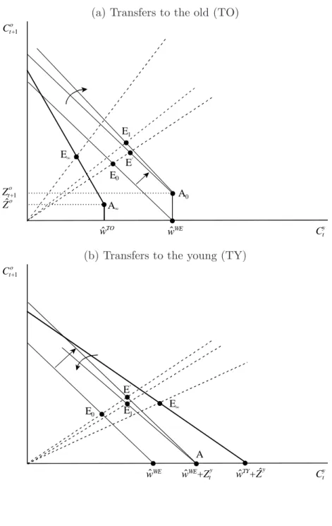
The first term in square brackets represents thedirect effect of the lump-sum transfer received in old age. Taken in isolation, this transfer expands the choice set and thus increases expected lifetime utility of shock-time newborns. The direct effect can be explained with the aid of Figure 3(a). The original budget line passes through E0, which is the initial equilibrium. The shock-time young anticipate transfers in old age equal to Z_t⁰₊₁. This shifts up the budget line in a parallel fashion.¹⁰ Holding constant the initially expected future interest rate, the optimal point shifts from E0 to E^′. But this is not the end of the story because it is only the partial equilibrium effect.

The second term in square brackets on the right-hand side of (29) represents the general equilibrium effect of the policy switch. It follows from (22) that the future capital stock is lower and the interest rate is higher as a result of the switch. In terms of Figure 3(a) the budget line pivots in a clockwise fashion around point A0 and optimal consumption moves from E^′ to E1. At impact the general equilibrium effect thus brings about a further expansion of the choice set faced by the shock-time young. Not surprisingly, therefore, the change in welfare at impact is unambiguously positive for such agents. In terms of Figure 2(b) the dash-dotted line lies above the dashed line at post-shock time τ = 0.

10Remember that agents are not allowed to borrow and that, therefore, consumption bundles withC_t^y> wt

Figure 3: Effect of government transfers in the exogenous growth model (a) Transfers to the old (TO)

!

! C_t+1^o

E₀

C_t^y E₄

!

!

!

Z_t+1^o

!

A₀ A₄

Zˆ^o

E₁

E^N

!

wˆ^TO wˆ^WE

(b) Transfers to the young (TY)

!

! C_t+1^o

E₀

C_t^y E₁

! wˆ^TY+Zˆ^y

! !

E₄

! ! E^N

wˆ^WE wˆ^WE+Z_t^y A

Before turning to the long-run welfare effects we first introduce the following lemma exploiting an important property of the factor-price frontier.

Lemma 1 [Implications of the factor price frontier] Assume that 0≤η < 1−α (exogenous growth model), the economy is initially in the steady state associated with the WE or TY scenario, and adopt Assumption 1 (ˆr > n, dynamic efficiency). Let dk_t+∞/dz_i denote the long-run effect on the capital intensity of a unit perturbation in z_i occurring at shock-time τ = 0 and evaluated at z_i = 0. It follows that the long-run effect on weighted factor prices can be written as:

Cˆ^o (1 + ˆr)²

drt+∞

dz_i +dwt+∞

dz_i = ∆dkt+∞

dz_i , (L1.1)

where ∆is a positive constant:

∆≡

η+α(1−α−η)rˆ−n 1 + ˆr

ˆr+δ

α >0. (L1.2)

Proof: See Heijdra et al. (2010, Appendix E).

The welfare effect experienced by future steady-state generations can be written as:

dEΛ^y_t+∞(z1) dz1

=U^′( ˆC^y)

π(1 +n)

1−π kˆ+ ∆dk_t+∞

dz1

T0, (30) where we have used Lemma 1 and note that lim_τ→∞k_t+τ = ˆk^TO. The first term in brackets represents the steady-state direct effect, which is positive. The second term comprises the general equilibrium effect, which is negative because capital is crowded out in the long run (see (22) above). On the one hand the reduction in the long-run capital intensity increases the interest rate which positively affects welfare. But on the other hand it also reduces the wage rate, which lowers welfare. In terms of Figure 3(a), the budget line shifts to the left because of the fall in the long-run wage ( ˆw^TO <wˆ^WE). In addition, long-run transfers are lower than anticipated transfers at impact ( ˆZ^o < Z_t^o₊₁) so that point A_∞ lies south-west from A0. The steady-state interest rate exceeds the future rate faced by shock-time newborns (ˆr^TO > r_t+1), i.e. the budget line is steeper than at impact. The steady-state equilibrium is at point E_∞.

Comparing columns (a) and (b) of Table 2 reveals that the long-run welfare effect of the policy switch is negative, i.e. the crowding out of capital induces a very strong reduction in

who are alive at the time of the shock, it is thus better to let the accidental bequests go to waste than to give them to the elderly. To better understand the intuition behind this remarkable result, we first state the following lemma on the key features of the steady-state first-best social optimum (FBSO).

Lemma 2 [Golden rules] Assume that 0≤η <1−α (exogenous growth model), and define steady-state welfare of a young agent (L2.1), the economy-wide resource constraint (L2.2), and the macroeconomic production function (L2.3) as follows:

EΛ^y ≡ U(C^y) +1−π

1 +ρU(C^o), (L2.1)

f(k)−(δ+n)k = C^y+ 1−π

1 +nC^o+g, (L2.2)

f(k) = Ω0k^α+η. (L2.3)

The social planner chooses non-negative values for C^y, C^o, k, and g in order to maximize EΛ^y subject to the constraints (L2.2)–(L2.3). In addition to satisfying the constraints the first-best social optimum has the following features:

U^′( ˜C^y)

U^′( ˜C^o) = 1 +n

1 +ρ, (S1)

f^′(˜k) = n+δ, (S2)

˜

g = 0. (S3)

Proof: See Heijdra et al. (2010, Appendix F).

Using the terminology of Samuelson (1968), we refer to requirement (S1) of the FBSO as the Biological-Interest-Rate Golden Rule (BGR), and to requirement (S2) as the Production Golden Rule (PGR). Of course, requirement (S3) just states that the social planner does not waste valuable resources.

Armed with Lemma 2 we can investigate the efficiency properties of the market economy.

In the decentralized equilibrium for the WE scenario the steady-state equilibrium satisfies the resource constraint (L2.2) as well as the following conditions:

U^′( ˆC^y)

U^′( ˆC^o) = (1−π) (1 + ˆr)

1 +ρ , (W1)

α

α+ηf^′(ˆk) = ˆr+δ, (W2)

ˆ

g = π(1 + ˆr) ˆk. (W3)