A behavioral economic approach to multiple job holdings with leisure

IHS Working Paper 23

September 2020

A behavioral economic approach to multiple job holdings with leisure

Jaroslava Hlouskova

Panagiotis Tsigaris

Author(s)

Jaroslava Hlouskova, Panagiotis Tsigaris Editor(s)

Robert M. Kunst Title

A behavioral economic approach to multiple job holdings with leisure

Institut für Höhere Studien - Institute for Advanced Studies (IHS) Josefstädter Straße 39, A-1080 Wien

T +43 1 59991-0 F +43 1 59991-555 www.ihs.ac.at ZVR: 066207973 Funder(s) FWF License

„A behavioral economic approach to multiple job holdings with leisure“ by Jaroslava Hlouskova, Panagiotis Tsigaris is licensed under the Creative Commons: Attribution 4.0 License (http://creativecommons.org/licenses/by/4.0/)

All contents are without guarantee. Any liability of the contributors of the IHS from the content of this work is excluded.

All IHS Working Papers are available online:

https://irihs.ihs.ac.at/view/ihs_series/ser=5Fihswps.html

This paper is available for download without charge at: https://irihs.ihs.ac.at/id/eprint/5428/

A behavioral economic approach to multiple job holdings with leisure. ^∗

Jaroslava Hlouskova

Macroeconomics and Economic Policy, Institute for Advanced Studies, Vienna, Austria Ecosystems Services and Management, International Institute for Applied Systems Analysis (IIASA),

Laxenburg, Austria

Department of Economics, Faculty of National Economy, University of Economics in Bratislava, Slovakia

Panagiotis Tsigaris

Department of Economics, Thompson Rivers University, Kamloops, BC, Canada

∗

The authors would like to thank Robert Kunst for very helpful comments that lead to improvement of the

paper. Jaroslava Hlouskova gratefully acknowledges financial support from the Austrian Science Fund FWF

(project number V 438-N32).

Abstract

Financial constraints or economic needs, career development, psychological satisfaction as well as demographic and situational factors cause workers to seek more than one job while enjoying leisure time. In this paper we examine how a worker with prospect theory type of preferences allocates her time between leisure, a safe job and a risky job. Optimal time allocation for a sufficient loss averse worker depends on the reference level which in turn determines whether the worker is willing to experience relative losses or not. When the reference level is relatively low then the sufficiently loss averse worker will allocate some of her time to leisure and will hold both jobs in order to diversify risk and reduce income loss arising from the risky job. However, if the probability of a good state of nature is very high and the reference level is very low, the worker spends time only on leisure and the risky job while avoids the safe job. Loss aversion does not affect the optimal time allocation to the three activities as the time allocation results in avoiding relative losses for any state of nature. When the reference level is relative high, but not too high, the worker will allocate her time between both safe and risky jobs as well as to the leisure. Worker with very high reference level will avoid the safe job and will divide her time between the risky job and the leisure. In both cases the worker is willing to accept relative losses in the bad state of nature provided it is compensated with relative gains in the good state of nature. Here the allocation of time to the three activities depends on the degree of loss aversion. When the reference level is relatively low, but not too low, an increase in the reference level will reduce leisure time, reduce time in the risky job and increase time in the safe job. At very low reference levels, an increase in the reference level will result in the worker re-allocating her time from leisure to the risky job assuming the probability of a good state of nature is higher than a threshold. When the reference level is high the opposite effects are observed. We also examine other comparative statics including the effect of changes in the wage rate.

Keywords: multiple job holdings, prospect theory, loss aversion

JEL classification: D81, G11, E24

1 Introduction

In many instances a worker will undertake more than one job due to financial constraints or needs, career development, psychological satisfaction as well as demographic and situational factors (Campion et al., 2020). Without discounting any of the above listed motivations, the important reason for multiple job-holding is financial constraints and economic needs. ¹ Workers often face a constraint on the number of hours available for them to work in their primary job limiting their earnings capacity (Shishko and Rostker, 1976; Dickey et al., 2015;

Hirsch et al., 2016b). This underemployment causes the individual to seek for another job in order to achieve the desired income goal. Income supplement from a second job due to earning constraints in the primary occupation is also a motivating factor (Hirsch et al., 2016a;

Klinger and Weber, 2020). Other motivations include unstable earnings in the primary job (e.g., artists, independent consultants, entrepreneurs) which cause people to diversify risk associated with income fluctuations by working also in more stable occupations such as an eight hour per day job (Throsby and Zednik, 2011; Guariglia and Kim, 2004; Hlouskova et al., 2017; Menger, 2017). Teachers and university professors who have a desired income goal higher than the salary often undertake a second job (Guthrie, 1969; Raffel and Groff, 1990; Parham and Gordon, 2011; Timothy and Nkwama, 2017). Some workers will moonlight because they enjoy the work reducing their leisure time (Averett, 2001; Amuedo-Dorantes and Kimmel, 2009). Some individuals undertake additional activities in the underground economy working in a second job under the table and evade having to pay payroll taxes (Brunet, 2008).

A second job might be taken for career development whereby the individual derives different utilities from the desire for diversity in the job’s tasks (Fraser and Gold, 2001; Renna and Oaxaca, 2006; Casacuberta and Gandelman, 2012; Hirsch et al., 2016a, 2016b) or a second job could aid the worker in transition to a new career (Arora, 2013; Russo et al., 2018).

In addition, a second job may be undertaken for personal satisfaction, passion, aspiration, enjoyment or for a new enrichment and experience (Averett, 2001; Osborne and Warren, 2006;

Wrzesniewski et al. 2013; Caza et al., 2018).

In this research we explore the role the loss aversion and reference dependent behavior play in deciding to take on multiple job-holdings. To this end, prospect theory will be used to explain the desire of workers to hold one or two jobs, one being the job with the safe income and the second one is considered to yield risky income (e.g., an entrepreneur) providing new insights that have not been previously explored when also leisure time is considered. ² An

1

Furthermore Campion et al. (2020) found that at least 5 percent of the working population in the US have multiple jobs and this can be as high as 35 percent. A study by Conen (2020) found similar participation rates in multiple job holdings for Europe. The trend is expected to increase in the future.

2

Economists attempt to study human behavior under risk using the expected utility theory (EUT) model developed by von Neumann and Morgenstern (1944) as a rational choice theory with stable and consistent preferences derived from well founded basic axioms. However, Kahneman and Tversky (1979) found in exper- imental laboratories that human behavior under risk violates the axioms and predictions of the EUT theory.

Kahneman and Tversky also developed a theoretical model of preferences, namely prospect theory, which is

example would be a hybrid entrepreneur (Campion et al., 2020) who is starting a new risky business but also works in a safe occupation with a known wage (Raffiee and Feng, 2014;

Thorgren et al., 2016; Schulz et al., 2017).

There is some evidence that workers use prospect theory type of preferences. For example, prospect theory has been used to explore labor supply decisions of New York City cab driver (Camerer et al., 1997). Camerer et al. (1997) find evidence that New York cab drivers work more (less) hours on a given day when the average hourly wage rate is low (high) on that day making this consistent with the predictions of prospect theory. Crawford and Meng (2011), based on the Koszegi and Rabin (2006) reference dependent model, found that drivers use hours and sometimes income targets as reference points. Farber (2005, 2008) also finds support that workers use prospect theory type of preferences.

As discussed in the introductory paragraph, a worker could be searching for a second job because her current earnings fall short relative to a target level. The target level is nothing else than a reference level and hence prospect theory analysis seems to be applicable. Workers could be loss averse as well. Loss aversion within the context of labour supply implies that workers are more sensitive when they experience a loss of income than when faced with an equal income gain. Loss of income can be caused by either hour constraints, wage reduction or a bad state of nature occurring (such as global pandemic of coronavirus disease, COVID-19).

According to prospect theory this loss of income results in more pain than the happiness from a gain of equal magnitude. Furthermore, workers could be displaying risk aversion in the domain of gains but become risk lovers when confronted with losses (diminishing sensitivity).

Thus, losses could trigger workers to search for a second risky job which yields an uncertain income.

In this paper we extend the model in Hlouskova et al. (2017) that is based on a behavioral portfolio approach. They present an explanation for workers, with prospect type of prefer- ences, to hold two jobs, one with safe income and the other with an uncertain income, while holding leisure time constant. In classical economic theory, the issue of incentive to work has often been analyzed as a choice between working and leisure time. Introducing leisure into the model is an obvious enrichment. Workers make their choices simultaneously by considering both the multiple holdings of jobs as well as the time they allocate towards leisure. In this research, we intend to explore the implications of this more general model.

Thus, in this paper, the model is extended to include leisure decisions. The worker now decides on how to allocate her time endowment between leisure, a safe job that pays with certainty a given wage rate and a risky job which pays an uncertain wage. For simplicity we assume two states of nature. A good state of nature where the worker can earn in the risky job a wage rate greater than that of the safe job and a bad state of nature where the wage

built on its own axioms and captures the evidence found in such laboratories such as reference dependent

behaviour, aversion against losses, diminishing sensitivity (risk aversion in domain of gains and risk seeking in

domain of losses). See also Barberis (2013).

rate is below the one she earns in the safe job. The wage rate in the bad state of nature is assumed to be nonzero and could be bounded by minimum wage laws. Two following cases arise. First, when worker’s actual income in either state of nature exceeds her reference level.

Namely, the worker prefers not to have relative losses in any state of nature which can be achieved by having a low reference level for income. Second, when worker’s actual income in the good state of nature exceeds the reference level, resulting in relative gains, but the actual income in the bad state of nature is less than the reference level and thus resulting in relative losses. The second case occurs for those workers that have a high income reference level (i.e., high income aspiration) and thus are willing to take more risk and accept relative losses in the bad state of nature for having relative gains in the good state of nature. ³

When the reference level is relatively low (but not very low) an increase in the reference level (aspiration) will reduce the time allocated to the risky job as well as the leisure, which is thus offset by an increase in the time allocated to the safe job. In Hlouskova et al. (2017) time allocated to the risky job also fell with an increase in the reference level but leisure was not allowed to adjust forcing only an increase in time allocated to the safe job. In this extension we also find that for very low reference levels, when assuming the probability of the good state of nature being sufficiently high and thus the risky job becomes more attractive, the worker will avoid the safe job totally and allocate time between the risky job and leisure.

In this case, an increase in the reference level will increase time allocated to the risky job taking away time from leisure. In the absence of leisure choice, this effect was not present in Hlouskova et al. (2017). For the optimal solution to evolve the worker has to be sufficiently loss averse but because the household remains in the domain of relative gains in both states of nature loss aversion does not affect the time allocation to the three activities. Any increase in any of the wage rates, say due to a lower payroll tax, will result in the worker being happier since expected utility increases. In the first case where all three activities are selected, an increase in the wage rate in the good or bad state of nature will increase time allocated to the risky job and decrease time allocated to both leisure and to the safe job. The effect of an increase in the wage rate in the safe job to the three activities is in general ambiguous due to the conflicting income and substitution effects. There would be, for instance, an increase in time allocated to the safe job and a reduction in the time allocated to the risky job and leisure if the probability of good state of nature to occur and the reference level for income are sufficiently low.

When the reference level is relatively high (but not too high) then the worker achieves a relative gain in the good state of nature and is willing to suffer a relative loss in the bad state of nature. In this case, an increase in the reference level yields opposite results to the previous case where the reference level was relatively low, except for the expected utility function which in all cases under consideration decreases with increasing reference level (depletion). Thus, an

3

There is a third possibility when the worker faces relative losses in both states of nature. However, her

expected utility is below the expected utility of one of the two other cases. See appendix A for further details.

increase in the reference level will increase the time allocated to the risky job and also leisure time, while such a change reduces the time allocation to the safe job. When the reference level is very high, the worker will avoid allocating time to the safe job, just like in the case when the reference level is very low. Thus, in the case of the very high reference level any further increases in the reference level will increase time allocated to the risky job by taking away time from leisure just like in the case with the very low reference level. Furthermore, when the reference level is relatively high, the optimal time allocated to the three activities depends on the loss aversion parameter. An increase in loss aversion will reduce time allocated to the risky job and leisure but will increase time allocation to the safe job. An increase in any wage rate is welcoming news to the worker as it increases expected utility (enrichment). In the case whereby the individual undertakes all three activities, an increase in the wage rate in the bad state of nature will increase time allocated to the risky job and the leisure. Offsetting these increases is a decrease in time allocated to the safe job. On the other hand, an increase in the wage rate in the good state of nature will reduce time in the risky activity if loss aversion is higher than a threshold, and unambiguously stimulate leisure time while the effect on time spent on the safe job is ambiguous. However, the effect of time spent in the risky job is also ambiguous for less loss averse workers. Finally, an increase in the wage rate in the safe job will reduce time in the risky job, reduce leisure and increase time in the safe job.

The next section presents the model. This is followed by describing the optimal solutions assuming a low reference level with comparative statics presented, including changes in the wage rate. Then optimal solutions with high reference level are explored with the corre- sponding comparative static analysis. Some concluding remarks are offered at the end of the paper.

2 Model

The model assumes that a hypothetical worker is deciding on the allocation of her time endowment, T > 0, towards a safe job in the amount of L ≥ 0, towards a risky job, J ≥ 0, and towards leisure time, E ≥ 0, such that L + J + E = T . The safe job yields the wage rate of w _a > 0. The risky job has an uncertain wage rate w and can yield w _g , a wage rate higher than that of the safe job, with probability p. However, it might also yield a lower wage rate of w _b > 0 with probability 1 − p. The lower wage rate w _b > 0 can be considered as a minimum wage rate regulated by the government. Hence, the wage rates are such that 0 < w _b < w a < w g . In addition, we assume that the expected wage of the risky job is higher than the wage of the safe job, i.e., E (w) = p w _g + (1 − p)w _b > w _a or p > ^w _w

^a

^{− w}

^b

g

− w

_b

≡ p _L , in order to induce the worker to undertake the second job which is more risky.

The worker has reference dependent preferences, i.e., when deciding about allocation of

time to the two different jobs and to leisure, she evaluates her final income as gains or losses

relative to a reference level, ˆ Y ≥ 0, to benchmark her final income and to derive her utility.

The reference level might have important implications as to how the worker will allocate her time to the three activities and also how she responds to changes in the exogenous variables.

Income earnings (and therefore consumption) from the two jobs, is given by Y _s = w _a L + w _s J, s ∈ {b, g}. Thus, the final income net of the reference level, Y _s − Y ˆ , i ∈ {b, g}, is uncertain and equals

Y _s − Y ˆ = w _a L + w _s J − Y ˆ = (w _s − w _a )J + w _a (T − E) − Y ˆ

The worker can earn w _a (T −E) with certainty by allocating (T −E) of her time to the safe job, but can make more earnings by taking the risky job if the good state of nature materializes.

The worker is assumed to maximize expectation of the following utility function that is the sum of the power utility of the leisure and the prospect theory value function ⁴

U (E, J) = E ^{1 − γ}

1 − γ + V (Y − Y ˆ ) (1)

where the value function V (·) is given as

V (Y − Y ˆ ) =



 



 



(Y − Y ˆ )

^1−γ

1 − γ , Y ≥ Y ˆ

−λ ^{( ˆ Y −} ₁ ^Y ₋ ⁾ _γ

^1−γ

, Y < Y ˆ

for λ > 1, with λ being the loss aversion parameter. Thus, the worker’s reduction in utility arising from a loss in her income is greater (in absolute terms) than the marginal utility from a gain in income (of the same size) near the reference level. This is thus consistent with the fact that workers are more sensitive to a (relative) loss in their income (i.e., income below their reference level) than when they experience relative gain (i.e., income above their reference level). Another feature of the S-shaped value function is that workers are risk averse in the domain of gains (preference for certain smaller gains over uncertain larger gains), but become risk seekers (risk lovers) in the domain of losses (preference for uncertain large losses over small certain losses).

Thus, the worker is assumed to choose the amount of time allocated to the risky job and leisure by solving

Max _(E,J) E (U (E, J)) = Max _(E,J) h

E

^1−γ

1 − γ + E (V (Y − Y ˆ )) i such that : Y − Y ˆ = (w − w _a )J + w _a (T − E) − Y ˆ

J, E ≥ 0, J + E ≤ T

(2)

4

We assume leisure enters the utility function separately and that leisure, like relative income, has a constant

diminishing sensitivity measured by γ. Although the preferences are restricted, they are commonly used in

economic models (see Bodie et al., 1992, among others).

Next sections shed more light on how time allocation among safe job, risky job and leisure depend on the size of the reference level of income for sufficiently loss averse worker.

3 Low reference levels

In this section we consider a worker that has relatively low reference levels and is sufficiently loss averse towards risk taking. There are two cases to consider. First, a relatively low reference level, such that max {0, w _L T } ≤ Y ˆ ≤ w _a T , which is described in proposition 1 below and second, even a lower reference level, such that ˆ Y < w _L T , if the probability of the good state to occur is sufficiently high. The solution of the latter case is given in proposition 2. Under proposition 1 a sufficiently loss averse worker will undertake the risky job with the hope it will increase its earnings while working also in the safe job diversifying further its risk.

The worker will allocate some time also to her leisure that is proportional to the maximum amount a worker can earn in the safe job net of the reference level. The amount of time the worker allocates to the risky job is proportional to the optimal leisure time.

Proposition 1 Let max {0, w _L T} ≤ Y ˆ ≤ w _a T and λ > max n

1 K

γ

,

w

a

k

2

γ o

, where K _γ , k ₂ and w L are given by (15), (18) and (19). Then problem (2) obtains its maximum at (J ^∗ , E ^∗ ) =

J ^{P 1} , E ^{P 1} where

J ^{P 1} = 1 − K ^1/γ w _a − w _b ·

k

w _a T − Y ˆ k

1 + K _γ ^1/γ + w _a

= 1 − K ^1/γ

w _a − w _b k E ^P1 , (3) E ^{P 1} = w _a T − Y ˆ

k

1 + K _γ ^1/γ + w _a

and (4)

L ^{P 1} = T − J ^{P 1} − E ^P1 (5)

with K and k being defined by (16) and (17).

Proof. The statement of the proposition follows directly from Appendix A, namely from (S1-P1), (S3-P2), (S5-P2) and (S2-P3).

Note that for ˆ Y < w _a T is 0 < J ^{P 1} , E ^{P 1} , L ^{P 1} < T . Note in addition that (54), (55) and (56) in Appendix A provide the explicit formulations of Y _g ^{P 1} , Y _b ^{P 1} and E U J ^{P 1} , J ^{P 1}

and imply that Y _g ^{P 1} > Y _b ^{P 1} > Y ˆ and E U J ^{P 1} , E ^{P 1}

> 0 when ˆ Y < w _a T . Note in addition that loss averse worker will avoid the risky job and leisure and thus allocate all her time to the safe job if her reference level coincides with the maximum earnings she can obtain from the safe job, i.e., when ˆ Y = w _a T .

Under proposition 2 below, the sufficiently loss averse worker, with a lower reference

level than that considered in proposition 1, allocates no time to the safe job. The optimal

time allocated to the risky job is expressed in an implicit form while the remaining time

is allocated to the leisure. Both solutions, time allocated to the risky job as well as time allocated to the leisure, are independent of worker’s degree of loss aversion but in order for such conditions to evolve and for the worker to take both jobs, she has to be sufficiently loss averse. Under proposition 1 the household has to have a loss aversion parameter such that λ > max n

1 K

γ

,

w

a

k

2

γ o

, while under proposition 2, when worker has even lower reference level for income, the loss aversion parameter must be λ >

w

a

k

2

γ

and the probability of the good state of nature high enough, namely p > p _U , in order to induce the worker to leave the safe job and undertake only the risky job.

Proposition 2 Let 0 ≤ Y < w ˆ _L T , λ >

w

a

k

2

γ

and p > p _U where w _L is given by (19) and p U is given by (24). Then problem (2) obtains its maximum at (J ^∗ , E ^∗ ) = J ^{P 1} , E ^{P 1}

where J ^{P 1} ∈ _ˆ

Y w

_b

, T

is the solution of

−(T − J ) ^{− γ} + p

w _g J − Y ˆ ⁻ γ

w _g + (1 − p)

w _b J − Y ˆ ⁻ γ

w _b = 0 (6)

E ^{P 1} = T − J ^{P 1} (7)

L ^P1 = 0 (8)

Proof. The statement of the proposition follows directly from the Appendix A, namely from (S2-P1), (S5-P2) and (S2-P3).

Note that w _L > 0 if and only if p > p _U . Note in addition that 0 < J ^{P 1} , E ^{P 1} < T , Y _g ^{P 1} = w _g J ^{P 1} > Y ˆ , Y _b ^{P 1} = w _b J ^{P 1} > Y ˆ and E U J ^{P 1}

is given by (79).

3.1 Reference level

Under proposition 1 an increase in the reference level will cause the amount of time allocated to the risky job and leisure to fall and thus more time is allocated to the safe job. On the other hand, in case when the worker does not undertake the safe job, i.e., when the reference level is even lower than the one stated in proposition 1, an increase in the reference level will stimulate interest to undertake more of the risky job while trading off some leisure time.

Under both proposition 1 and proposition 2 the impact of an increase in the reference level reduces relative gains in both states of nature and leads to a lower expected utility.

3.2 Time endowment

Under proposition 1 an increase in the time endowment will increase leisure time and also

time allocated to the risky job. The impact on the safe job depends on the value of the

probability of the good state of nature from occurring. If the probability is relatively low

then the additional time will also be allocated to the safe job while if the probability of the

good state of nature is high then time allocated to the safe job will fall. Under proposition

2, whereby the worker does not hold a safe job, an increase in time endowment will increase time allocated to the risky job and to leisure (as in proposition 1). In both cases an increase in time endowment is welcome news to the worker in that relative gains in both states of nature increase and so does expected utility.

3.3 Wage rates

An increase in the wage rate of the risky job in either the bad state or the good state of nature under proposition 1 will cause an increase in time allocated to the risky job, a decline in leisure time and time allocated to the safe job, an increase in relative gains in the good state of nature and a decline in relative gains in the bad state of nature but overall an increase in happiness ⁵ as the effect of an increase in relative gains in the good state of nature is stronger than the decline in relative gains in the bad state of nature and the decline in the leisure.

Under proposition 2, the effect of an increase in the wage rate in either the bad state or the good state is ambiguous for risky job, leisure and relative gains. Namely, an increase of the wage of the risky job will increase time allocated to the risky job, reduce leisure time with no effect on the safe job only when the already low reference level is below a certain threshold level. Relative gains in both states of nature will increase only if the low reference level is lower than the threshold level. The opposite dynamics applies when the reference level exceeds a threshold level. However, expected utility will increase within this low reference level.

An increase in the wage rate of the safe job under proposition 1 has ambiguous effects on the time allocated to the risky and safe job due to the conflicting income and substitution effects. Ambiguous is also the effect on leisure and relative gains in the good state of nature but there is an increase in relative gains in the bad state of nature which is sufficient enough to increase expected utility. Leisure activity will increase if the probability of the good state of nature is higher than a threshold or if the threshold level is sufficiently high. For proposition 2 a change in the wage rate of the safe job has no effect on the decision variables. On the other hand, if the probability of the good state to occur and the income reference levels are sufficiently low then, under proposition 1, an increase in the wage rate of the safe job stimulates the interest to undertake more of the safe job while trading off time allocated to the risky job and leisure time.

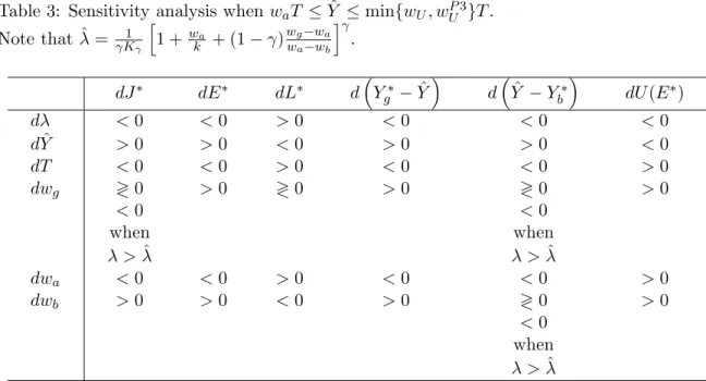
Tables 1 and 2 summarize the sensitivity results related to propositions 1 and 2 which have been discussed above.

5

By happiness we understand the indirect utility function.

Table 1: Sensitivity analysis when max{0, w _L T } ≤ Y ˆ ≤ w _a T , ˆ Y _T = ^{(1 − γ)(} _γw ^{− w}

^L

^)w

^a

^T

a

− w

L

.

dJ ^∗ dE ^∗ dL ^∗ d

Y _g ^∗ − Y ˆ

d

Y _b ^∗ − Y ˆ

dU (E ^∗ )

dλ = 0 = 0 = 0 = 0 = 0 = 0

d Y ˆ < 0 < 0 > 0 < 0 < 0 < 0

dT > 0 > 0 ≷ 0 > 0 > 0 > 0

> 0 for p < p _U

< 0 for p > p _U

dw _g > 0 < 0 < 0 > 0 < 0 > 0

dw _a ≷ 0 ≷ 0 ≷ 0 ≷ 0 > 0 > 0

> 0 for p > p _U

or for p < p _U

Y > ˆ Y ˆ _T

< 0 < 0 > 0 < 0

p < p _U p < p _U p < p _U p < p _U Y < ˆ Y ˆ T Y < ˆ Y ˆ T Y < ˆ Y ˆ T Y < ˆ Y ˆ T

dw _b > 0 < 0 < 0 > 0 < 0 > 0

4 High reference levels

The next two propositions present solutions to problem (2) when the reference level is set at relatively high level. In proposition 3 the reference level is such that is exceeds the threshold level w _a T , i.e., ˆ Y > w _a T , but it is below another threshold level as described in proposition 3. Finally, proposition 4 presents results for largest reference levels up to w _g T . Proposition 3 has explicit solution of all three activities undertaken and worker thus allocates non-zero time to both jobs and leisure. Unlike for lower values of the reference level, for higher values of reference level for income, the solution, i.e., time allocation towards risky job, safe job and leisure, depends on the worker’s degree of loss aversion. The optimal solution for leisure is proportional to the reference level net of the maximum amount the worker can earn in the safe job and time allocated to the risky job is proportional to the leisure time (as in the case with the low reference level).

Proposition 3 Let w _a T < Y ˆ ≤ min

w _U , w ^P _U ³ T and λ > max n λ ^{P 2} ,

h (w

g

− w

a

) ˆ Y (w

g

T − Y ˆ )k

2

i γ o

, where

k ₂ , w _U , w ^P _U ³ and λ ^{P 2} are given by (18), (20), (21) and (22). Then problem (2) obtains its

Table 2: Sensitivity analysis when ˆ Y < w _L T and p > p _U = ^w

^a

^{− w}

^b

(w

g

− w

a

)

wbwg

γ

+w

a

− w

b

. Note that ˆ Y _U = w _b J ^∗ − [(1 − p)w _b (w _g − w _b )]

^1+γ1

(T − J ^∗ ), ˆ Y _U,w

_g

= (1 − γ)w _g J ^∗

dJ ^∗ dE ^∗ dL ^∗ d

Y _g ^∗ − Y ˆ

d

Y _b ^∗ − Y ˆ

dU(E ^∗ )

dλ = 0 = 0 = 0 = 0 = 0 = 0

d Y ˆ > 0 < 0 = 0 < 0 < 0 < 0

when when

Y < ˆ Y ˆ _U Y < ˆ Y ˆ _U

dT > 0 > 0 = 0 > 0 > 0 > 0

dw _g ≷ 0 ≶ 0 = 0 ≷ 0 ≷ 0 > 0

> 0 < 0 > 0 > 0

when when when when

Y < ˆ Y ˆ _U,w

_g

Y < ˆ Y ˆ _U,w

_g

Y < ˆ Y ˆ _U,w

_g

Y < ˆ Y ˆ _U,w

_g

< 0 > 0 < 0 < 0

when when when when

Y > ˆ Y ˆ _U,w

_g

Y > ˆ Y ˆ _U,w

_g

Y > ˆ Y ˆ _U,w

_g

Y > ˆ Y ˆ _U,w

_g

dw _a = 0 = 0 = 0 = 0 = 0 = 0

dw _b ≷ 0 ≶ 0 = 0 ≷ 0 ≷ 0 > 0

> 0 < 0 > 0 > 0

when when when when

Y < ˆ Y ˆ _U,w

_b

Y < ˆ Y ˆ _U,w

_b

Y < ˆ Y ˆ _U,w

_b

Y < ˆ Y ˆ _U,w

_b

< 0 > 0 < 0 < 0

when when when when

Y > ˆ Y ˆ _U,w

_b

Y > ˆ Y ˆ _U,w

_b

Y > ˆ Y ˆ _U,w

_b

Y > ˆ Y ˆ _U,w

_b

maximum at (J ^∗ , E ^∗ ) = J ^{P 2} , E ^{P 2} where

J ^P2 = 1 + (λK ) ^1/γ w _a − w _b ·

k

Y ˆ − w _a T

k h

(λK _γ ) ^1/γ − 1 i

− w _a

= 1 + (λK ) ^1/γ

w _a − w _b k E ^{P 2} (9) E ^P2 = Y ˆ − w _a T

k h

(λK _γ ) ^1/γ − 1 i

− w _a

(10)

L ^{P 2} = T − J ^P2 − E ^{P 2} (11)

with K _γ , K and k being define by (15), (16) and (17).

Proof. The statement of the proposition follows directly from the Appendix A, namely from (S4-P1), (S1-P2) and (S1-P3).

Note that 0 < J ^{P 2} , E ^{P 2} , L ^{P 2} < T . Note in addition that (98), (99) and (100) in Appendix A provide the explicit formulations of Y _g ^{P 2} , Y _b ^{P 2} and E U J ^{P 2} , J ^{P 2}

and imply that Y _g ^{P 2} >

Y ˆ , Y _b ^{P 2} < Y ˆ and E U J ^{P 2} , E ^{P 2}

< 0.

For the largest values of income reference levels the worker allocates her time among the risky job and leisure while she avoids completely the safe job (similar to proposition 2 which presents results for the lowest values of reference levels). The following proposition presents results for this case and the optimal time allocated to the risky job is expressed in the implicit form.

Proposition 4 Let max

w _U , w _U ^{P 3} T ≤ Y ˆ ≤ w _g T and λ > λ ^P2 , where w _U , w ^P _U ³ and λ ^{P 2} are given by (20), (21) and (22). Then problem (2) obtains its maximum at (J ^∗ , E ^∗ ) = J ^{P 2} , E ^P2 where J ^{P 2} ∈ _ˆ

Y w

g

, T

is the solution of

−(T − J ) ^{− γ} + p

w _g J − Y ˆ ⁻ γ

w _g + λ(1 − p)

Y ˆ − w _b J ⁻ γ

w _b = 0 (12)

E ^{P 2} = T − J ^{P 2} (13)

L ^{P 2} = 0 (14)

Proof. The statement of the proposition follows directly from Appendix A, namely from (S4-P1), (S2-P2) and (S3-P3).

Note that 0 < J ^{P 2} , E ^{P 2} < T . Note in addition that Y _g ^{P 2} = w _g J ^{P 2} > Y ˆ , Y _b ^{P 2} = w _b J ^{P 2} <

Y ˆ and E U J ^{P 2}

is given by (130).

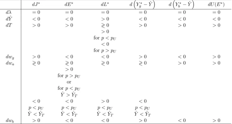
Comparative static analysis is shown in table 3 for proposition 3 and table 4 for proposition 4.

4.1 Loss Aversion

Under proposition 3 an increase in a worker’s degree of the loss aversion (λ) makes the risky job and leisure less attractive while increases the attractiveness towards the safe job. There is a reduction in relative gains in the good state of nature as well as in relative losses in the bad state of nature and happiness level declines as well. Thus, a marginal reduction in the loss averse parameter can lead to increase happiness.

We do not report sensitivity analysis of solutions with respect to the degree of loss aversion for reference levels such that max{w _U , w _U ^P3 }T < Y ˆ ≤ w _g T , as both w _U and w _U ^P3 are increasing functions in λ, such that lim (w U ) _λ → + ∞ = lim w _U ^{P 3}

λ → + ∞ = w _g . This and proposition 3 imply that for w _a T < Y ˆ ≤ w _g T the following holds

lim J _λ ^∗ → + ∞ = Y ˆ − w _a T w _g − w _a lim E _λ ^∗ → + ∞ = 0

lim L ^∗ _λ → + ∞ = w _g T − Y ˆ

w _g − w _a

Thus, an extremely loss averse worker has a tendency to decrease leisure time to zero and allocate its time between the safe job and the risky job.

4.2 Reference level

An increase in the reference level, when the reference level is already relatively high to start with, will cause an increase in the time allocated to the risky job, an increase in leisure time and a reduction in time allocated to the safe job which is the opposite to the case when the worker has a relatively low reference level (proposition 1). At even higher reference level, as in proposition 4, we observe a trade-off between time allocated between risky job and leisure time. Namely an increase in the reference level leads to an increase in time allocated to the risky job and a reduction in leisure time (table 4). Table 3 also shows that an increase in the reference level will increase relative gains in the good state of nature as well as the relative losses in the bad state of nature. An increase in relative losses has the strongest effect on the level of worker’s happiness which decreases with increasing reference level. At the highest reference levels (proposition 4) an increase in the reference level will increase relative gains in the good state of nature but reduce relative losses in the bad state of nature. As an increase in reference level for income leads to a reduction in happiness also in this case, then this is caused by the reduction of time allocated to the leisure.

4.3 Time Endowment

Under proposition 3 an increase in time endowment will increase time allocated in the safe job but reduce time allocated in the risky job and leisure (as in case when the degree of loss aversion was increased). An increase in the time endowment will reduce relative gains in the good state of nature as well as relative losses in the bad state of nature but increase expected utility, which is thus caused by the reduction of relative losses in the bad state of nature. Under proposition 4 the worker uses the increased time endowment for more leisure time while time allocated to the risky job decreases. Relative gains in the good state of nature fall and relative losses in the bad state of nature increase. As indirect utility function (happiness) increases with increased time endowment then this is caused by increased time to leisure. Note that these effects are in opposite direction than effects caused by the change in the reference level.

4.4 Wage Rates

Under proposition 3 an increase in the wage rate in the good state of nature has an ambiguous

effect on time allocated to the risky job. However, for sufficiently large degree of loss aversion

is time allocated to the risky job reduced which is opposite to the effect it had when the

reference level was low (proposition 1). Leisure time will increase, while time allocated in the

safe job is also ambiguous. Relative gains in the good state of nature will increase while effect on relative losses is again ambiguous. However, if loss aversion is above the threshold level then relative losses will decrease. Note that an increase of any wage rate increases indirect utility (happiness). Under proposition 3 an increase in the wage rate in the bad state of nature will increase the time allocated to the risky job and to leisure while reducing the time allocated to the safe job. Relative gains increase in the good state of nature while again the effect on relative losses is ambiguous but they also increase provided loss aversion exceeds certain threshold level. An increase in the wage rate of the safe job under proposition 3 will reduce time allocated to the risky job, reduce leisure time and increase time allocated in the safe job. Relative gains in the good state of nature will fall as well as relative losses in the bad state of nature which has stronger effect than decline in leisure time and in relative gains (in good state of nature) as happiness increases with increased wage rate of the safe job.

The following holds for a sufficiently loss averse worker with highest reference level, as stated in proposition 4. An increase in the wage rate in the good state of nature will increase time allocated to the risky job, reduce leisure, increase relative gains in the good state of nature and decrease relative losses in the bad state of nature if the reference level is sufficiently high.

An opposite comparative statics applies when the reference level is somehow smaller. An increase in the wage rate in the bad state of nature will unambiguously reduce time allocated to the risky job and increase leisure time (which has the main effect on the increase of the happiness level), decrease relative gains in the good state of nature and increase relative losses in the bad state of nature. This might look counter-intuitive (that an increase of the wage rate of the risky job in the bad state of nature decreases time allocated into the risky job.

However, utility function of the worker with prospect theory based preferences implies, see

(1), that the leisure time enters her utility function separately and thus has a strong role in

determining her happiness level. Note that happiness level will increase with an increase in

the wage rates in either the good or bad state of nature. Finally, an increase in the wage rate

in the safe job has no effect on the decision variables since the worker allocates her time only

to the risky job and leisure.

Table 3: Sensitivity analysis when w _a T ≤ Y ˆ ≤ min{w _U , w ^P _U ³ }T . Note that ˆ λ = _γK ¹

γ

h

1 + ^w _k

^a

+ (1 − γ ) ^w _w

^g

^{− w}

^a

a

− w

b

i γ

.

dJ ^∗ dE ^∗ dL ^∗ d

Y _g ^∗ − Y ˆ

d

Y ˆ − Y _b ^∗

dU (E ^∗ )

dλ < 0 < 0 > 0 < 0 < 0 < 0

d Y ˆ > 0 > 0 < 0 > 0 > 0 < 0

dT < 0 < 0 > 0 < 0 < 0 > 0

dw _g ≷ 0 > 0 ≷ 0 > 0 ≷ 0 > 0

< 0 < 0

when when

λ > λ ˆ λ > λ ˆ

dw _a < 0 < 0 > 0 < 0 < 0 > 0

dw _b > 0 > 0 < 0 > 0 ≷ 0 > 0

< 0 when λ > λ ˆ

Table 4: Sensitivity analysis when max{w _U , w ^P _U ³ }T ≤ Y ˆ ≤ w _g T and when λ is sufficiently large.

dJ ^∗ dE ^∗ dL ^∗ d

Y _g ^∗ − Y ˆ

d

Y ˆ − Y _b ^∗

dU (E ^∗ )

d Y ˆ > 0 < 0 = 0 > 0 < 0 < 0

dT < 0 > 0 = 0 < 0 > 0 > 0

dw _g ≷ 0 ≶ 0 = 0 ≷ 0 ≶ 0 > 0

> 0 < 0 > 0 < 0

when when when when

Y > ˆ Y ˆ _U,w

_g

Y > ˆ Y ˆ _U,w

_g

Y > ˆ Y ˆ _U,w

_g

Y > ˆ Y ˆ _U,w

_g

< 0 > 0 < 0 > 0

when when when when

Y < ˆ Y ˆ _U,w

_g

Y < ˆ Y ˆ _U,w

_g

Y < ˆ Y ˆ _U,w

_g

Y < ˆ Y ˆ _U,w

_g

dw _a = 0 = 0 = 0 = 0 = 0 = 0

dw _b < 0 > 0 = 0 < 0 > 0 > 0

5 Conclusion

Workers who face financial constraints or an economic need or have aspirations for belonging

in an income group, engage in holding more than one job. In this paper a positive analysis

is conducted to determine the role of the reference level and loss aversion in the allocation of

time to leisure, a safe and a risky job. The worker has a choice to make decisions based on

whether she wants to face relative losses in any state of nature. If the worker is interested in avoiding relative losses then she has a low reference level for her income and allocates time between the three activities in such a way that she avoids these losses in any state of nature.

Leisure time under such case is a normal good and work effort is inferior as it is normally in a neoclassical setting. However, in the case whereby the worker has a high reference level, say high aspirations to belong to a higher income class, leisure becomes an inferior good while work effort is now normal. Changes in the reference level thus have implications in terms of re-allocation of time between the activities. At low reference level and when time is allocated to all three activities an increase in the reference level will reduce leisure, reduce time allocated in the risky job and increase time allocated in the safe job. But when the reference level is high and the worker allocates her time across all three activities, an increase in the reference level will increase leisure, increase time allocated to the risky job and reduce time allocated in the safe job. An increase in the wage rate of the safe job, say due to lower taxes, is inconclusive in terms of stimulating time allocated to the safe job when the reference level is low. This is due to the conflicting income and substitution effects that are in operation. But when the reference level is high and work effort is normal then the income and substitution effects operate in the same direction and time allocated to the safe job increases with an increase in the wage rate of the safe job while time is taken away from leisure and the risky job. An increase in the wage rate in the bad state of nature stimulates time allocated to the risky job under most cases without any additional conditions. Assuming that the wage rate in the bad state of nature is bounded by minimum wage laws then an increase in the minimum wage rate can lead to increasing time allocation to the risky job but can come at the expense of time allocated to the safe job and leisure time when the reference level for income is low.

This paper is focussed on a positive analysis and did not look into normative issues.

There are a number of potential extensions that are worthwhile undertaking. One can force

the worker’s time allocated to the safe job to be less than the optimal due to constraints

on the number of hours available for her to work in her safe job and analyze the impact

this has on decision to hold more than one job. Another extension is to introduce a wage

tax and autonomous taxes and conduct a differential incidence analysis. A wage tax yields

similar results to a reduction in wage rate that has been explored in this paper but equally an

increase in autonomous taxes can be seen as a reduction in the reference level which impacts

have been analyzed in this paper as well. Hence, a budget balanced analysis whereby the

government say reduces the wage tax but increases autonomous taxes to make up for the loss

of tax revenue and seeing the effects of such a policy change on time allocation and happiness

is worth exploring.

References

[1] Amuedo-Dorantes, C. and J. Kimmel, 2009. Moonlighting over the business cycle, Eco- nomic Inquiry, 47, 754–765.

[2] Arora, N., 2013. Analyzing moonlighting as HR retention policy: A new trend, Journal of Commerce and Management Thought, 4, 329–338.

[3] Averett, S.L., 2001. Moonlighting: Multiple motives and gender differences, Applied Economics, 33, 1391–1410.

[4] Barberis, N., 2013. Thirty years of prospect theory in economics: A review and assess- ment, Journal of Economic Perspectives, 27, 173–196.

[5] Brunet, J.R., 2008. Blurring the line between public and private sectors: The case of police officers’ off-duty employment, Public Personnel Management, 37, 161–174.

[6] Campion, E.D., B.B. Caza and S.E. Moss, 2020. Multiple jobholding: An integrative systematic review and future research agenda, Journal of Management, 46, 165–191.

[7] Camerer, C., L. Babcock, G. Loewenstein and R. Thaler, 1997. Labor supply of New York City cabdrivers: One day at a time, Quarterly Journal of Economics, 112, 407–441.

[8] Casacuberta, C. and N. Gandelman, 2012. Multiple job holding: The artist’s labour supply approach, Applied Economics, 44, 323–337.

[9] Caza, B.B., S. Moss and H. Vough, 2018. From synchronizing to harmonizing: The process of authenticating multiple work identities, Administrative Science Quarterly, 63, 703–745.

[10] Conen, W.S., 2020. Multiple jobholding in Europe: Structure and dynamics, WSI Study;

No. 20, HansBockler-Stiftung.

[11] Crawford, V. and J. Meng, 2011. New York City cab drivers’ labor supply revisited:

Reference-dependent preferences with rational expectations targets for hours and income, American Economic Review, 101, 1912–1932.

[12] Dickey, H., V. Watson and A. Zangelidis, 2015. What triggers multiple job-holding? A state preference investigation, Discussion paper no. 15-4, Centre for European Labour Market Research, Aberdeen, UK.

[13] Farber, H., 2005. Is tomorrow another day? The labor supply of New York City cab- drivers, Journal of Political Economy, 113, 46–82.

[14] Farber, H., 2008. Reference-dependent preferences and labor supply: The case of New

York City taxi drivers, American Economic Review, 98, 1069–1082.

[15] Fraser, J. and M. Gold, 2001. Portfolio workers: Autonomy and control amongst freelance translators, Work, Employment and Society, 15, 679–697.

[16] Guariglia, A. and B.-Y. Kim, 2004. Earnings uncertainty, precautionary saving, and moonlighting in Russia, Journal of Population Economics, 17, 289–310.

[17] Guthrie, W.H., 1969. Teachers in the moonlight, Monthly Labour Review, 92, 28–31.

[18] Hirsch, B., M.M. Husain and J.V. Winters, 2016a. Multiple job holding, local labor markets, and the business cycle, IZA Journal of Labor Economics, 5, 4–33.

[19] Hirsch, B., M.M. Husain and J.V. Winters, 2016b. The puzzling fixity of multiple job holding across regions and labor markets, Discussion paper no. 9631, Institute for the Study of Labor (IZA), Bonn, Germany.

[20] Hlouskova, J., P. Tsigaris, A. Caplanova and R. Sivak, 2017. A behavioral portfolio approach to multiple job holdings, Review of Economics of the Household, 15, 669–689.

[21] Kahneman, D. and A. Tversky, 1979. Prospect theory: An analysis of decision under risk, Econometrica, 47, 363–391.

[22] Klinger, S. and E. Weber, 2020. Secondary job holding in Germany, Applied Economics, 52, 3238–3256.

[23] Koszegi, B. and M. Rabin, 2006. A model of reference-dependent preferences, Quarterly Journal of Economics, 121, 1133–1165.

[24] Menger P.M., 2017. Contingent high-skilled work and flexible labor markets. Creative workers and independent contractors cycling between employment and unemployment 1, Swiss Journal of Sociology, 43, 253–284.

[25] von Neumann, J. and O. Morgenstern, Theory of Games and Economic Behavior, Princeton University Press, 1944.

[26] Osborne, R. and J. Warren, 2006. Multiple job holding: A working option for young people, Labor, Employment and Work in New Zealand, 377–384.

[27] Parham, N.J. and S.P. Gordon, 2011. Moonlighting: A harsh reality for many teachers, Phi Delta Kappan, 92, 47–51.

[28] Raffel, J. A. and L.R. Groff, 1990. Shedding light on the dark side of teacher moonlight- ing, Educational Evaluation and Policy Analysis, 12, 403–414.

[29] Raffiee, J. and J. Feng, 2014. Should I quit my day job? A hybrid path to entrepreneur-

ship, Academy of Management Journal, 57, 936–963.

[30] Renna, F. and R.L. Oaxaca, 2006. The economics of dual jobholding: A job portfolio model of labor supply, IZA discussion paper no. 1915, Institute for the Study of Labor (IZA), Bonn, Germany.

[31] Russo, G., I. Fronteira, T.S. Jesus and J. Buchan, 2018. Understanding nurses’ dual practice: A scoping review of what we know and what we still need to ask on nurses holding multiple jobs, Human Resources for Health, 16, 14–30.

[32] Schulz, M., D. Urbig and V. Procher, 2017. The role of hybrid entrepreneurship in ex- plaining multiple job holders’ earnings structure, Journal of Business Venturing Insights, 7, 9–14.

[33] Shishko, R. and B. Rostker, 1976. The economics of multiple job holding, American Economic Review, 66, 298–308.

[34] Timothy, V. L. and S. Nkwama, 2017. Moonlighting among teachers in urban Tanzania:

A survey of public primary schools in Ilala District, Cogent Education, 4, 1–8.

[35] Thorgren, S., C. Siren, C. Nordstrom and J. Wincent, 2016. Hybrid entrepreneurs’

second-step choice: The nonlinear relationship between age and intention to enter full- time entrepreneurship, Journal of Business Venturing Insights, 5, 14–18.

[36] Throsby, D. and A. Zednik, 2011. Multiple job-holding and artistic careers: Some em- pirical evidence, Cultural Trends, 20, 9–24.

[37] Wrzesniewski, A., N. LoBuglio, J.E. Dutton and J.M. Berg, 2013. Job crafting and cul-

tivating positive meaning and identity work, Advances in Positive Organizational Psy-

chology, 1, 281–302.

Appendix A

Let us introduce the following notation

K _γ = (1 − p)(w a − w _b ) ^{1 − γ}

p (w _g − w _a ) ^{1 − γ} (15)

K = (1 − p)(w _a − w _b )

p (w _g − w _a ) (16)

k =

"

w _a p

w g − w _b w _a − w _b

1 − γ # 1/γ

(17)

k ₂ =

"

w _a (1 − p)

w _g − w _b w _g − w _a

1 − γ # 1/γ

= kK _γ ^1/γ (18)

w L = w _b − w _g K ^1/γ

1 − K ^1/γ + ^w

^a

⁻ _k ^w

^b

(19)

w _U = w _U (λ) = w _b + w _g (λK ) ^1/γ

1 + (λK ) ^1/γ + ^w

^a

⁻ _k ^w

^b

(20)

w ^P _U ³ = w ^P _U ³ (λ) = w _g 1 + ^w _λ

^g_1/γ

^{− w} _k

^a

2

(21)

λ ^{P 2} = 1

K _γ ^1/γ + w _a k ₂

! γ

(22) ˆ λ = 1

γK _γ

1 + w _a

k + (1 − γ) w _g − w _a w _a − w _b

γ

(23) p _U = w _a − w _b

(w _g − w _a )

w

_b

w

g

γ

+ w _a − w _b

(24)

Note that w _U (λ) and w ^P _U ³ (λ) are increasing functions in λ and lim(w _U ) _λ → + ∞ = lim(w _U ^{P 3} ) _λ → + ∞ = w _g . The following holds

d dw _g k

K _γ ^1/γ + 1

= 1 − γ γ

k w _g − w _b

1 − K ^1/γ

> 0 for p > p _L (25) d

dw _g k h

(λK _γ ) ^1/γ − 1 i

= − 1 − γ γ

k w _g − w _b

h 1 + (λK ) ^1/γ i

< 0 (26)

d dw _g k

h

1 + (λK) ^1/γ i

= k

γ (w _g − w _b )

1 − γ + (1 − γ )(w _g − w _a ) − (w _g − w _b )

w _g − w _a (λK ) ^1/γ

< 0 for λ > 1 K γ

d

dw _g k = 1 − γ γ

k

w _g − w _b > 0 (27)

d dw g

k ₂ = − 1 − γ γ

k

w g − w _b K ^1/γ < 0 (28)

d

dw _g (k + k ₂ ) = 1 − γ γ

k w _g − w _b

1 − K ^1/γ

> 0 for p > p _L (29) d

dw _g K ^1/γ = − 1 γ

K ^1/γ

w _g − w _a (30)

d

dw _g K _γ ^1/γ = − 1 − γ γ

K ^1/γ

w _a − w _b (31)

d

dw _b k = 1 − γ γ

k w _g − w _b

w _g − w _a

w _a − w _b > 0 (32)

d dw _b k

K _γ ^1/γ + 1

= 1 − γ γ

k w _g − w _b

1 − K ^1/γ

w _g − w _a

w _a − w _b > 0 for p > p L (33) d

dw _b K ^1/γ = − 1 γ

K ^1/γ

w _a − w _b (34)

d

dw _b K _γ ^1/γ = − 1 − γ γ

K _γ ^1/γ

w _a − w _b = − 1 − γ γ

w _g − w _a

(w _a − w _b ) ² K ^1/γ (35) d

dw _b

1 − K ^1/γ k

w _a − w _b = 1 − K ^1/γ k γ(w _a − w _b ) ²

"

K ^1/γ

1 − K ^1/γ + w _g − w _a + γ(w _a − w _b ) w _g − w _b

#

(36) d

dw _b k h

(λK _γ ) ^1/γ − 1 i

= − 1 − γ γ

k w _g − w _b

(λK _γ ) ^1/γ − w _g − w _a w _a − w _b

< for λ > 1 K _γ

w g − w a

w _a − w _b γ

(37) d

dw _b

1 + (λK ) ^1/γ

w a − w _b k = k

γ(w a − w _b )(w g − w _b )

w _g − w _b

w a − w _b − (1 − γ)

1 + (λK) ^1/γ (38) d

dw _a K _γ ^1/γ = 1 − γ γ

w g − w _b

(w _g − w _a )(w _a − w _b ) K _γ ^1/γ (39) d

dw _a K ^1/γ = 1 γ

w _g − w _b

(w _g − w _a )(w _a − w _b ) K ^1/γ (40)

d

dw _a k = k γ

γw _a − w _b

w _a (w _a − w _b ) (41)

d dw _a k

1 + K _γ ^1/γ

= k

γw _a

γw _a − w _b

w _a − w _b + w _g − γw _a w _g − w _a K _γ ^1/γ

= k

γw _a (w _a − w _b ) h

γw _a

1 − K ^1/γ

+ w _g K ^1/γ − w _b i d

dw _a k h

(λK _γ ) ^1/γ − 1 i

= k

γw _a

w _g − γw _a

w _g − w _a (λK _γ ) ^1/γ − γw _a − w _b w _a − w _b

d dw a

k w a

h (λK _γ ) ^1/γ − 1 i

= 1 − γ γ

k w ² _a (w a − w _b )

h

w _g (λK) ^1/γ + w _b i

> 0 d

dw _a k

w _a − w _b = − w _b

γw _a (w _a − w _b ) ² k (42)

d dw _a

1 − K ^1/γ k

w _a − w _b = − k γw _a (w _a − w _b ) ²

w _b + w _g (w _a − w _b ) w _g − w _a K ^1/γ

(43) d

dw _a K ^1/γ k

w _a − w _b = kK ^1/γ w _g

γw _a (w _a − w _b )(w _g − w _a ) > 0 (44) d

dw _a h

1 + (λK ) ^1/γ i k

w _a − w _b = k γw _a (w _a − w _b ) ²

w _g (w _a − w _b )

w _g − w _a (λK ) ^1/γ − w _b

(45) There are three cases to consider:

(P1) ˆ Y ≤ Y _b ≤ Y _g (P2) Y _b ≤ Y ˆ ≤ Y _g (P3) Y _b ≤ Y _g ≤ Y ˆ

The proofs are conducted in such a way that for each of the three cases the corresponding problem is formulated and maximum (maxima) of each problems are compared among them- selves and the largest one is the maximum of (2).

Note in addition that for ˆ Y ≤ w _a T is point

J = 0, E = T − _w ^{Y ˆ}

a

feasible for all three cases/problems as then Y _g = Y _b = ˆ Y . The value of the corresponding utility function is

T −

^Yˆ

wa

1−γ

1 − γ .

Problem (P1):

Max _(J,E) : E (U (J, E)) = ^E ₁

^1−γ

_{− γ} + p [ (w

g

− w

a

)J+w

a

(T − E) − Y ˆ ]

^1−γ

1 − γ + (1 − p) [ ⁻ (w

a

− w

b

)J +w

a

(T − E) − Y ˆ ]

^1−γ

1 − γ

such that : Y ˆ ≤ w _a (T − E) − (w _a − w _b )J J + E ≤ T

J, E ≥ 0



 

 

 

 

 

 

 

  (P1)

Note that the necessary condition for feasibility is that ˆ Y ≤ w _a T . ⁶

6

This follows from Y

_b

≥ Y ˆ and thus from ˆ Y ≤ w

a

(T − E) − (w

a

− w

_b

)J.