Risk assessment with regard to the occurrence of malaria in Africa under
the influence of observed and projected climate change
I n a u g u r a l - D i s s e r t a t i o n zur
Erlangung des Doktorgrades
der Mathematisch-Naturwissenschaftlichen Fakultät der Universität zu Köln
vorgelegt von
Volker Ermert aus Kirchen/Sieg
Köln 2010
Dr. A. P. Morse Tag der mündlichen Prüfung: 23. November 2009
Abstract
Malaria is one of the most serious health problems in the world. The projected climate change will probably alter the range and transmission potential of malaria in Africa. In this study, potential changes in the malaria transmission are assessed by forcing three malaria models with bias-corrected data from ensemble scenario runs of a state-of-the- art regional climate model.
The Liverpool Malaria Model (LMM) from the Geography Department of the Uni- versity of Liverpool is utilised. The LMM simulates the spread of malaria at a daily resolution using daily mean temperature and 10-day accumulated precipitation. The simulation of some key processes has been modified in the model, in order to reflect a more physical relationship. An extensive literature survey with regard to entomologi- cal and parasitological malaria variables enables the calibration and validation of a new LMM version. Comparison of this version with the original model exhibits marked improvements. The new version demonstrates a realistic simulation of entomological variables and of the malaria season, as well as correctly reproduces the epidemic poten- tial at fringes of endemic malaria areas. Various sensitivity experiments reveal that the LMM is fairly sensitive to values of its required parameters. Effects of climatic changes on the malaria season are additionally verified by the MARA Seasonality Model (MSM).
The Garki model finally enables the completion of the malaria picture in terms of the immune status and the infectiousness of different population groups, as well as relative to the age-dependent prevalence structure.
In every case three ensemble runs were performed on a 0.5◦ grid. The LMM was driven for the present-day climate (1960-2000) by bias-corrected data from the REgional MOdel (REMO), with a land use and land cover specified by the Food and Agriculture Organization (FAO). Malaria projections were carried out for 2001-2050 according to the climate scenarios A1B and B1 as well as FAO land use and land cover changes. Garki model runs were subsequently forced by the Entomological Inoculation Rate (EIR) from the LMM. Finally, additional results relative to the malaria season were produced by MSM.
For the present-day climate (1960-2000), the highest biting rates are simulated for Equatorial Africa. The malaria runs show a decrease in the malaria spread from Central Africa towards the Sahel. The length of the malaria season is closely related to monsoon
rainfall. The model simulations show a marked influence of mountainous areas causing a complex pattern of the spread of malaria in East Africa. The malaria infected popula- tion reveals the expected peak in children below an age of about five years. Regions of epidemic malaria occurrence, as defined by the coefficient of variation of the annual par- asite prevalence maximum, are found along a band in the northern Sahel. Farther south, malaria occurs more regularly and is therefore characterised as endemic. Epidemic- prone areas are additionally identified at various highland territories, as well as in arid and semi-arid zones of the Greater Horn of Africa. No adequate immune protection of the population was found for these areas.
Largely due to land surface degradation, REMO simulates a prominent surface warm- ing and a significant reduction in the annual rainfall amount over most of tropical Africa in either climate change scenario. Assuming no future human-imposed constraints on malaria transmission, changes in temperature and precipitation will alter the future ge- ographic distribution of malaria. In the northern part of sub-Saharan Africa, the preci- pitation decline will force significant decreases of the malaria transmission in the Sahel.
In addition to the withdrawal of malaria transmission along the fringe of the Sahara, the frequency of malaria occurrence will be reduced for several grid boxes of the Sahel. As a result, epidemics in these more densely populated areas will become more likely, in par- ticularly as adults lose their immunity. The level of malaria prevalence farther south will remain stable for most areas. However, the start of the malaria season will be delayed and the transmission is expected to cease earlier.
Most pronounced changes in Africa are found for East Africa. Significantly higher temperatures and slightly higher rainfall cause a substantial increase in the season length and parasite prevalence in formerly epidemic-prone areas. Territories formerly unsuit- able for malaria will become suitable under the warmer future climate. The simulations indicate changes in the highland epidemic risk. At most grid boxes malaria transmission will stabilise below about 2000 m. At these altitudes the population will improve their immune status. In contrast, malaria will climb to formerly malaria-free zones above these levels enforcing the probability of malaria epidemics.
Zusammenfassung
Die Malaria stellt eine der gefährlichsten Krankheiten der Welt dar. Höchstwahrschein- lich werden sich die Ausbreitung und das Übertragungspotenzial der Malaria in Afrika unter dem Einfluss des projizierten Klimawandels verändern. Aus diesem Grund ver- sucht die vorliegende Studie potenzielle Veränderungen in der Malariaübertragung abzu- schätzen. Drei unterschiedliche Malariamodelle werden hierzu mit korrigierten Ensem- bleläufen eines auf dem Stand der Wissenschaft befindlichen regionalen Klimamodells betrieben.
Verwendung findet zunächst das sog. „Liverpool Malaria Model (LMM)“ vom Geo- graphischen Department der Universität Liverpool. Das LMM simuliert die Verbreitung der Malaria auf Tagesbasis und wird lediglich durch die Tagesmitteltemperatur und die 10-tägig akkumulierte Niederschlagsmenge angetrieben. Um Vorgänge in der Natur bes- ser widerzuspiegeln wurde im LMM die Simulierung einiger wichtiger Prozesse ver- ändert. Eine intensive Literaturrecherche in Bezug auf entomologische und parasitolo- gische Malariavariablen ermöglicht die Kalibrierung und die Validierung einer neuen LMM Version. Der Vergleich dieser neuen Version mit dem ursprünglichen Modell of- fenbart deutliche Verbesserungen. Die neue Modellversion zeigt eine realistische Simu- lation von entomologischen Variablen, der Malariasaison und reproduziert korrekt das Epidemiepotenzial am Rande endemischer Malariagebiete. Zahlreiche Sensitivitätsstu- dien zeigen, dass das LMM sensitiv bzgl. unterschiedlichen Modelleinstellungen rea- giert. Zusätzlich wird der Effekt der Klimaänderung auf die Malariasaison mit Hilfe des sog. „MARA Seasonality Models (MSM)“ überprüft. Durch die Berücksichtung des Immunstatus und der Infektiösität von unterschiedlichen Bevölkerungsgruppen als auch der altersabhängigen Struktur der Malariaprävalenz durch das sog. Garki Modell wird schließlich das Malariabild vervollständigt.
Die Modelle wurden jeweils für drei Ensembleläufe auf einem 0.5◦Gitter betrieben.
Für das heutige Klima (1960-2000) wurde das LMM hierbei mit korrigierten Daten des REgionalen MOdells (REMO) laufen gelassen, die wiederum auf einer Landnutzung und Landoberfläche der „Food and Agriculture Organization (FAO)“ beruhen. Malaria- projektionen wurden anschließend für den Zeitraum 2001-2050 mit REMO-Daten der Klimaszenarien A1B und B1 berechnet. In diesem Fall sind die Klimaszenarien durch FAO-Szenarien der Landnutzung und Landoberflächen entstanden. Danach wurde das
Garki Modell mit Hilfe der entomologischen Inokulationsrate des LMM betrieben. Zu- sätzliche Ergebnisse bezüglich der Malariasaison wurden schließlich durch das MSM produziert.
Für das heutige Klima (1960-2000) werden die höchsten Stechraten für das äqua- toriale Afrika simuliert. Die Malarialäufe zeigen einen Abfall in der Malariaverbreitung von Zentralafrika bis zum Sahel. Hierbei steht die Länge der Malariasaison im engen Zusammenhang mit dem Auftreten des Monsuns. Die ostafrikanischen Hochländer ver- ursachen außerdem ein komplexes Muster in der Malariaverbreitung. Wie erwartet treten in den ersten fünf Lebensjahren die höchsten Malariaprävalenzen auf. Epidemieregionen werden durch den Variationskoeffizienten der maximalen jährlichen Malariaprävalenz definiert. Solche Gebiete sind entlang eines Streifens im nördlichen Sahel zu finden.
Weiter südlich tritt die Malaria regelmäßiger auf und ist deshalb als endemisch cha- rakterisiert. Epidemiegebiete werden ebenso für zahlreiche Hochländer sowie für aride und semi-aride Regionen des Großen Horns von Afrika identifiziert. Für diese Gebiete konnte kein angemessener Immunschutz in der Bevölkerung gefunden werden.
In den REMO-Simulationen verursacht hauptsächlich die Degradation der Land- oberfläche in beiden Klimaszenarien einen deutlichen Temperaturanstieg und eine si- gnifikante Reduzierung der Jahresniederschläge über großen Teilen tropischen Afri- kas. Falls der Mensch die Malariaverbreitung in der Zukunft nicht merklich beeinflusst wird der Klimawandel die zukünftige Malariaübertragung stark verändern. Der Nieder- schlagsrückgang wird eine signifikante Reduzierung der Malariaübertragung im Sahel verursachen. Zusätzlich zum Rückzug der Malaria entlang der Grenze zur Sahara wird an einigen Gitterpunkten im Sahel die Häufigkeit des Malariaauftretens herabgesetzt. Diese bevölkerungsreicheren Gebiete werden somit häufiger mit Epidemien rechnen müssen, da in diesen Regionen vor allem Erwachsene ihre Immunität verlieren werden. Weiter südlich bleibt das Malarianiveau für die meisten Gebiete stabil, allerdings wird sich der Start der Malariasaison verzögern und es wird ein früheres Ende der Malariaübertragung erwartet.
In Afrika werden die stärksten Veränderungen für Ostafrika projiziert. In früheren Epidemiegebieten verursachen signifikant höhere Temperaturen und leicht erhöhte Nie- derschläge einen beträchtlichen Anstieg in der Länge der Saison und in der Prävalenz des Malariaparasiten. In Regionen die zuvor für die Malaria ungeeignet waren kann sich die Malaria in einem wärmeren zukünftigen Klima verbreiten. Die Simulationen offenbaren deutliche Veränderungen des Epidemierisikos der Hochländer. Für die meis- ten Gitterboxen stabilisiert sich unterhalb von etwa 2000 m die Malariaübertragung. In diesen Höhenbereichen wird die Bevölkerung eine bessere Immunität aufweisen. Das Risiko für Malariaepidemien steigt jedoch oberhalb dieses Niveaus, da die Malaria in diese Höhenlagen zukünftig erstmals vordringen kann.
Contents
Abstract i
Zusammenfassung iii
Abbreviations xi
Symbols xiii
1 Introduction 1
2 State of research, objectives, and overview 5
2.1 The Climate of Africa . . . 5
2.1.1 The climate of West Africa . . . 6
2.1.2 The climate of the Greater Horn of Africa . . . 7
2.1.3 Interannual variability of precipitation . . . 10
2.2 IPCC SRES scenarios . . . 14
2.3 Climate change projections . . . 16
2.3.1 Global climate projections . . . 16
2.3.2 Regional climate projections for Africa . . . 17
2.4 Malaria biology . . . 21
2.4.1 The parasite cycle . . . 21
2.4.2 Immunity . . . 23
2.4.3 Superinfection . . . 25
2.4.4 Parasite clearance . . . 25
2.4.5 Detectability of malaria parasites. . . 25
2.4.6 Heterogeneous biting . . . 26
2.5 Distribution of malaria transmission . . . 26
2.6 Malaria factors . . . 28
2.6.1 Climatic factors . . . 28
2.6.2 Other factors . . . 30
2.7 Malaria modelling. . . 32
2.7.1 Classic malaria models and successors . . . 32
2.7.2 Malaria models related to environmental variables . . . 33
2.7.3 Climate- and weather-driven malaria models . . . 35
2.8 Changes in malaria occurrence . . . 37
2.8.1 Observed malaria changes . . . 37
2.8.2 Projected malaria changes . . . 38
2.9 Objectives and Overview . . . 41
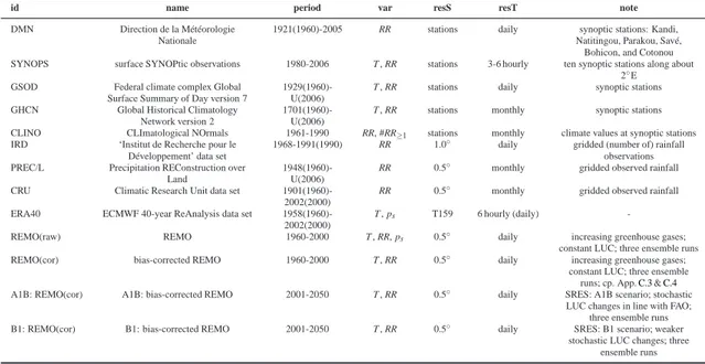
3 Data 45 3.1 DMN precipitation data . . . 45
3.2 Synoptic station data . . . 45
3.3 GSOD . . . 47
3.4 CLImatological NOrmals (CLINO) . . . 47
3.5 GHCN . . . 48
3.6 The ‘Institut de Recherche pour le Développement’ data set (IRD) . . . 49
3.7 PREC/L . . . 50
3.8 The Climatic Research Unit data set (CRU) . . . 51
3.9 The ECMWF 40-year ReAnalysis data set (ERA40) . . . 52
3.10 Present-day runs and climate projections from REMO . . . 53
3.10.1 REMO simulations . . . 53
3.10.2 Land use and land cover changes. . . 54
3.11 Entomological and parasitological data. . . 55
3.12 Data overview . . . 56
4 Validation of meteorological model data 57 4.1 REMO precipitation versus IRD . . . 57
4.1.1 Monthly and annual rainfall . . . 57
4.1.2 Frequency distribution of 10-day accumulated precipitation . . 60
4.2 REMO precipitation versus CRU . . . 62
4.3 ERA40 temperatures vs. station data . . . 64
4.4 REMO temperatures vs. station data . . . 66
4.5 REMO temperatures vs. ERA40 . . . 67
5 Malaria modelling 69
CONTENTS vii
5.1 Liverpool Malaria Model (LMM). . . 69
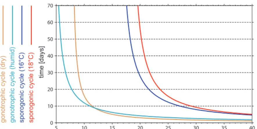
5.1.1 Gonotrophic cycle . . . 70
5.1.2 Egg deposition . . . 73
5.1.3 Mosquito Mature Age (MMA) . . . 76
5.1.4 Survival of immature mosquitoes . . . 76
5.1.5 Survival probability of adult mosquitoes (pd) . . . 78
5.1.6 Dry season survival of the mosquito population . . . 82
5.1.7 Sporogonic cycle . . . 83
5.1.8 Human blood index (a) . . . 84
5.1.9 Mosquito-to-human transmission efficiency (b) . . . 85
5.1.10 Human Infectious Age (HIA) . . . 86
5.1.11 Recovery rate (r) . . . 87
5.1.12 Gametocyte prevalence (sPR) . . . 88
5.1.13 Human-to-mosquito transmission efficiency (c) . . . 89
5.1.14 Issues regarding the age-dependence of malaria . . . 89
5.2 Garki model . . . 90
5.3 MARA Seasonality Model (MSM) . . . 95
6 Calibration, validation, and sensitivity tests of the LMM 97 6.1 LMM calibration and validation . . . 97
6.1.1 Calibration of the LMM . . . 98
6.1.2 Validation of the final LMMnsetting. . . 103
6.2 LMM sensitivity tests . . . 105
6.3 LMMnversus LMMo . . . 112
7 Malaria simulations for the present-day and future climate 117 7.1 REMO climate projections for Africa . . . 117
7.2 Present-day malaria distribution . . . 119
7.2.1 LMMnruns based on IRD/ERA40 (1968-1990) . . . 119
7.2.2 Evaluation of LMMnruns based on REMO (1960-2000) . . . . 122
7.2.3 Garki model simulations based on LMMnruns (1960-2000) . . 131
7.2.4 Malaria seasonality from the MSM (1960-2000) . . . 134
7.3 Malaria projections for 2001-2050 . . . 137
7.3.1 LMMnprojections based on REMO . . . 137
7.3.2 Garki model projections based on LMMn . . . 146
7.3.3 MSM projection of the malaria seasonality . . . 151
7.3.4 A1B versus B1 . . . 152
8 Summary, discussion, and future prospects 153
8.1 Summary . . . 153
8.2 Discussion and future prospects . . . 155
8.2.1 Calibration and sensitivity of the LMMn . . . 156
8.2.2 Performance of the malaria models . . . 157
8.2.3 Uncertainty of the applied climate projections . . . 159
8.2.4 Evaluation of the malaria projections . . . 160
8.2.5 Neglected factors and future extensions of the LMM . . . 162
8.2.6 Final remarks . . . 164
Appendices I
C Data processing . . . I C.1 Configuration of GSOD time series . . . I C.2 Generation of time series at synoptic stations . . . III C.3 Bias-correction of REMO precipitation . . . IV C.4 Bias-correction of REMO temperatures . . . VI C.5 The ensemble mean. . . VI C.6 The 360-day year . . . VII C.7 Grid transformation. . . VII C.8 The Wilcoxon-Mann-Whitney rank-sum test . . . VIII D Entomological and parasitological malaria variables . . . XI
D.1 Human biting ratio (HBR) . . . XII D.2 Circumsporozoite protein rate (CSPR) . . . XII D.3 Entomological inoculation rate (EIR) . . . XII D.4 Asexual parasite ratio (PR) . . . XIII D.5 Malaria seasonality . . . XIII D.6 Data table convention. . . XV D.7 Entomological and parasitological data . . . XVII D.8 Parasitological data assigned to synoptic stations . . . XXVIII D.9 Entomological data assigned to synoptic stations . . . XXIX D.10 Duration of the gonotrophic cycle (ng) . . . XXX D.11 Produced eggs per female mosquito (#Ep) . . . XXXI D.12 Development of immature mosquitoes . . . XXXII D.13 Daily survival probability of adult mosquitoes (pd) . . . XXXIV D.14 Sexual Parasite Ratio (sPR) . . . XXXVII D.15 Human-to-mosquito transmission efficiency (c) . . . XLI
D.16 Mosquito-to-human transmission efficiency (b) . . . XLII D.17 Human Blood Index (a) . . . XLIII D.18 Human Infectious Age (HIA) . . . XLIV E LMM validation and settings . . . XLV
E.1 Definition of the validation . . . XLV E.2 Figures and tables with regard to the LMM calibration . . . XLVII E.3 Figures in terms of the LMMnvalidation . . . LII E.4 Figures in terms of the LMMovalidation . . . LIV E.5 Spin-up period of the LMM . . . LVII F Supplementary figures . . . LVIII
F.1 Data from CRU . . . LVIII F.2 Standardised rainfall anomalies . . . LVIII F.3 Monthly REMO temperature and precipitation data . . . LIX F.4 Present-day malaria seasonality . . . LXVII F.5 Malaria projections . . . LXIX G Geographical information . . . LXXXVII
Glossary LXXXIX
References XCVII
Acknowledgements CXI
Erklärung CXIII
Lebenslauf CXV
Abbreviations
pd . . . daily survival probability of female mosquitoes [%]
An. . . Anopheles P. . . Plasmodium
AEJ . . . African Easterly Jet AEW . . . African Easterly Wave
AOGCM . . . Atmospheric Ocean General Circulation Model CH4 . . . methane
CLIMAT . . . monthly CLIMATological data, i.e. the WMO format 71 CLIMEX . . . CLIMatic indEX
CLINO . . . CLImatological NOrmals for the period 1961-1990 CO2 . . . carbon dioxide
CRU . . . Climatic Research Unit
DDT . . . Dichlor-Diphenyl-Trichloroethane
DMN . . . National Weather Service (French: ‘Direction de la Météorologie Nationale’)
DWD . . . German Weather Service (German: „Deutscher WetterDienst“) ECHAM4 . . . European Centre HAmburg Model, 4th generation
ECHAM5/MPI-OM European Centre HAmburg Model, 5th generation/Max-Planck- Institute-Ocean Model
ECMWF . . . European Centre for Medium-Range Weather Forecasts EEA . . . Equatorial East Africa
ERA40 . . . ECMWF 40-year ReAnalysis FAO . . . Food and Agriculture Organization GCM . . . General Circulation Model
GFDL-CM2.0 . . . . Geophysical Fluid Dynamics Laboratory Climate Model, version 2.0 GHCN . . . Global Historical Climatology Network version 2
GHG . . . GreenHouse Gas
GSOD . . . Federal climate complex Global Surface Summary of Day ver- sion 7
IMPETUS . . . Integrated Approach to the Efficient Management of Scarce Wa- ter Resources in West Africa, German: „Integratives Management Projekt für Einen Tragfähigen Umgang mit Süßwasser“
IOD . . . Indian Ocean Dipole
IPCC . . . Intergovernmental Panel on Climate Change IPCC-AR4 . . . Fourth Assessment Report of the IPCC
IRD . . . ‘Institut de Recherche pour le Développement’
ITCZ . . . InterTropical Convergence Zone ITF . . . InterTropical Front
LMM . . . Liverpool Malaria Model
LMMn . . . new Liverpool Malaria Model (see Sec.5.1)
LMMo . . . original Liverpool Malaria Model (Hoshen and Morse 2004) LUC . . . Land Use and land Cover
MARA . . . mapping MAlaria Risk in Africa MDM . . . MARA Distribution Model
MIASMA . . . Modelling framework for the health Impact ASsessment of Man- induced Atmospheric changes
MIROC3.2 medres Model for Interdisciplinary Research on Climate, medium-resolution version 3.2
MOZ . . . Malaria potential Occurrence Zone MRI . . . Meteorological Research Institute MRR . . . Mark-Release Recapture
MSM . . . MARA Seasonality Model N2O . . . nitrous oxide
NDVI . . . Normalised Difference Vegetation Index NeA . . . Northeast Africa
PCR . . . Polymerase Chain Reaction
PREC/L . . . Precipitation REConstruction over Land
QT-NASBA . . . QuanTitative-Nucleic Acid Sequence-Based Amplification RCM . . . Regional Climate Model
REMO . . . REgional MOdel
REMO(cor) . . . bias-corrected REMO data REMO(raw) . . . raw (uncorrected) REMO data
RT-PCR . . . Reverse Transcriptase-Polymerase Chain Reaction SOx . . . sulphur oxides
SRES . . . Special Report on Emission Scenarios SST . . . Sea-Surface Temperature
SYNOP . . . surface SYNOPtic observation, i.e. the WMO format 12 TEJ . . . Tropical Easterly Jet
VC . . . Vectorial Capacity
WHO . . . World Health Organization
WMO . . . World Meteorological Organization
Symbols
#Eo . . . number of oviposited eggs per female mosquito [eggs]
#Ep . . . number of produced eggs per female mosquito [eggs]
#RR≥1,m . . . monthly number of days with at least 1 mm precipitation
∆x . . . difference with regard to variable x between different periods or scenarios
ηd,¬RR . . . rainfall independent daily survival probability of immature mosquitoes [%]
ηd . . . daily survival probabilities of immature mosquitoes (field condi- tions) [%]
σ(x) . . . standard deviation in terms of variable x θ . . . potential temperature [◦C]
θ850 . . . potential temperature at 850 hPa [◦C]
a . . . Human Blood Index [%]
b . . . mosquito-to-human transmission efficiency [%]
c . . . human-to-mosquito transmission efficiency [%]
ca→c . . . adult-to-child conversion rate
cv(x) . . . coefficient of variation in terms of variable x CAP . . . CAP on the number of fertile mosquitoes CSPR . . . CircumSporozoite Protein Rate [%]
CSPRa . . . annual mean circumsporozoite protein rate [%]
DgH . . . degree days of the gonotrophic cycle (humid conditions) [◦days]
DgL . . . degree days of the gonotrophic cycle (dry conditions) [◦days]
Ds . . . degree days of the sporogonic cycle [◦days]
E2Seas . . . End month of the second malaria Season
EIR . . . Entomological Inoculation Rate, i.e. the number of infectious mosquito bites per human per time [infective bites time−1]
EIRa . . . annual Entomological Inoculation Rate [infective bites year−1] EIRm . . . monthly Entomological Inoculation Rate [infective bites month−1] EIRc . . . Entomological Inoculation Rate for children between 2-10 years
[infective bites time−1]
ESeas . . . End month of the malaria Season
f . . . fuzzy suitability (fuzzy distribution model) GF . . . Gametocyte Fraction
HBR . . . Human Biting Rate, i.e. the number of mosquito bites per human and per time period [bites time−1]
HBRa . . . annual Human Biting Rate [bites year−1]
HBRc . . . Human Biting Rate for children between 2-10 years [bites time−1] HIA . . . Human Infectious Age [days]
I . . . proportion of immune individuals
Ia . . . annual mean proportion of immune individuals MMA . . . Mosquito Mature Age [days]
MSeas . . . length of the Main malaria Season, i.e. the number of months in which 75% of EIRais recorded
n♂♀ . . . duration of gametocytogenesis [days]
nf . . . number of female mosquitoes
ng . . . duration of the gonotrophic cycle [days]
nm . . . duration of gametocyte maturation np . . . duration of the prepatent period [days]
ns . . . duration of the sporogonic cycle [days]
pd↓ . . . shift off relative to the dry season mosquito survival probability [%]
PR . . . asexual Parasite Ratio [%]
PR2−10 . . . annual mean asexual parasite ratio of children aged 2-10 years [%]
PRa . . . annual mean asexual parasite ratio [%]
PRmax,a . . . annual maximum of the asexual parasite ratio [%]
PRmin,a . . . annual minimum of the asexual parasite ratio [%]
R . . . daily larval development Rate [day−1] r . . . daily human recovery rate [day−1] R0 . . . basic Reproduction rate
RR− . . . 10-day accumulated rainfall threshold [mm]
RR3m . . . three-month moving averaged monthly precipitation (two preced- ing and the actual month are used) [mm]
RR• . . . rainfall laying multiplier
RRΣ10d . . . 10-day accumulated precipitation, i.e. the decadal precipitation amount [mm]
RRa . . . annual precipitation amount [mm]
RRc . . . catalyst month of precipitation RRm . . . monthly precipitation amount [mm]
S . . . most suitable rainfall condition in terms of egg deposition and sur- vival of immature mosquitoes (fuzzy distribution model) [mm]
S2Seas . . . Start month of the second malaria Season
SAR . . . Ratio between the Sexual and Asexual parasite prevalence, i.e. the proportion of gametocytaemic parasite positive humans [%]
ABBREVIATIONS AND SYMBOLS xv SARa . . . annual mean ratio between the sexual and asexual parasite preva-
lence [%]
SC(x) . . . skill score with regard to variable x
Seas . . . length of the malaria Season, i.e. the number of months suitable for malaria transmission
sPR . . . sexual parasite ratio, i.e. the gametocyte prevalence, which is the percentage of humans with gametocytes in their blood [%]
sPRa . . . annual mean sexual parasite ratio [%]
SSeas . . . Start month of the malaria Season T . . . daily mean temperature [◦C]
T3m . . . three-month moving average temperature (two preceding and the actual month are included)[◦C]
Ta . . . annual mean temperature [◦C]
TgH . . . temperature threshold of the gonotrophic cycle (humid conditions) [◦C]
TgL . . . temperature threshold of the gonotrophic cycle (dry conditions) [◦C]
Tmin,m . . . monthly minimum temperature [◦C]
Tm . . . monthly mean temperature [◦C]
Ts . . . sporogonic temperature threshold [◦C]
Tw . . . water temperature [◦C]
trim . . . trickle of the number of added infectious mosquitoes [infectious females (ten days)−1]
U1 . . . lower threshold of unsuitable rainfall conditions for egg deposition and survival of immature mosquitoes (fuzzy distribution model) [mm]
U2 . . . upper threshold of unsuitable rainfall conditions for egg deposition and survival of immature mosquitoes (fuzzy distribution model) [mm]
X2Seas . . . second identified month of maximum transmission (only available for a timeframe)
X Seas . . . month of maXimum transmission, i.e. the month with the largest EIR value
y . . . proportion of malaria positive individuals, i.e. the ‘true’ parasite prevalence
y1,a . . . annual mean proportion of malaria positive, infectious, non-immune individuals
y1 . . . proportion of malaria positive, infectious, non-immune individuals ya . . . annual mean proportion of malaria positive individuals
ymax,a . . . annual maximum proportion of malaria positive individuals z . . . altitude [m]
1 Introduction
The climate system of the Earth strongly affects human life and has a wide range of health impacts. Humans strongly affect the climate by GreenHouse Gas (GHG) emis- sions leading to anthropogenic global warming. It is well known that a warm and hu- mid climate triggers several water-associated diseases such as malaria (e.g., Githeko et al. 2000). Vector-borne diseases are highly sensitive to global warming and asso- ciated changes in precipitation (Martens et al. 1997). Malaria is particularly strongly influenced by warm and moist tropical atmospheric conditions (e.g., Patz et al. 1998).
Temperatures in Africa lie above the threshold for parasite development and rainy sea- sons lead to a rapid increase of the mosquito population (e.g., Hay et al. 2000a). The International Panel on Climate Change (IPCC) expects that climate change will have a mixed effect on the spread of malaria (Confalonieri et al. 2007). Like in the Sahel the geographical range will probably contract, elsewhere like in highlands it will expand, and the transmission season might be significantly altered. Populations at margins of current distribution are estimated to be particularly vulnerable to changes (Confalonieri et al. 2007).
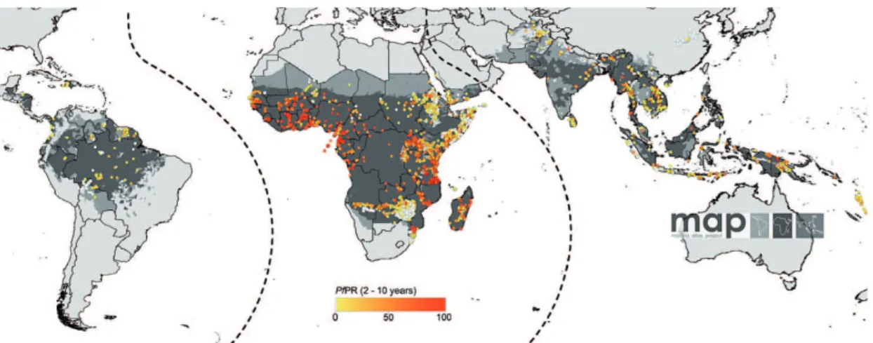
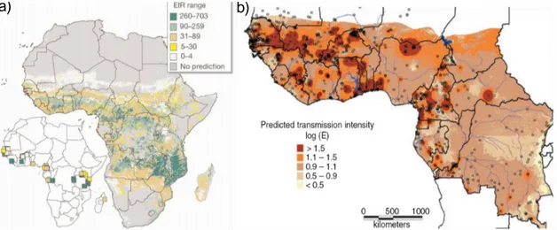
Fig. 1.1: Spatial limits of P. falciparum malaria risk. Areas are defined as stable (dark grey areas), unstable (medium grey areas), or malaria-free (light grey). Single dots display standardised community surveys of P. falciparum prevalence in children aged 2-10 years between January 1985 and July 2008 (for further information cf. Hay et al. 2009).
Malaria (Italian: ‘mal’=bad, ‘aria’=air) is caused by a parasitic protozoa of genus Plasmodium (P.) and is one of the world’s most serious health problems (e.g.,De Sav-
igny and Binka 2004). The World Health Organization (WHO) estimated that about two billion people, that is more than 40% of the total world population, are exposed to this mosquito-borne disease (WHO 1997; cp. Fig.1.1). Estimates revealed that malaria causes about 273 million clinical cases and 1.12 million deaths annually. At least 90%
of worldwide malaria deaths occur in sub-Saharan Africa (Greenwood and Mutabingwa 2002;Greenwood et al. 2005). This life-threatening disease is mostly restricted to young children as immunity to severe malaria is later developed (Gupta et al. 1999;Snow et al.
1999a). Pregnant women are especially prone to malaria causing an increased risk of infant low birth weight and infant mortality (Menendez 1999;Steketee and Mutabingwa 1999;D’Alessandro 1999).
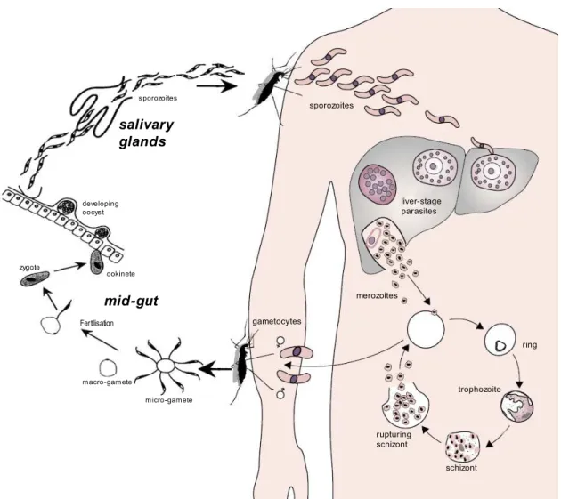
Anopheles (An.) is a genus of mosquito from the family Culicidae comprising sev- eral hundred recognised species. Female Anopheles require proteins for their egg pro- duction. Some of these species prefer to blood-feed on humans (anthropophily), while others preferentially feed on animals (zoophily). A few tens of Anopheles species are commonly malaria vectors and transmission takes place when either the mosquito fe- male or the human host is carrying malaria agents. Primarily responsible for malaria in Africa is the clinical meaningful and most dangerous pathogen P. falciparum (e.g.,Snow et al. 1997).
Most important malaria vectors in sub-Saharan Africa are found in the An. gambiae complex, also termed An. gambiae sensu lato (s.l.). Distribution of these vectors like that of An. gambiae sensu stricto (s.s.) and An. arabiensis is strongly governed by atmo- spheric conditions (Lindsay and Birley 1996;Lindsay et al. 1998). An. arabiensis, for example, was predominantly found in dry areas such as the Sahel, whereas An. gambiae sensu stricto (s.s.) tends to favour more humid environments such as in the tropical rainforest zone.
Malaria is a severe human disease with a striking positive correlation to poverty. En- demic malaria countries have lower rates of economic growth than non-malaria countries (Nabarro and Tayle 1998;Sachs and Malaney 2002;Greenwood et al. 2005). Malaria impedes development, is related to lack of work, and forces income loss. People suffer- ing from malaria often struggle to earn their living. Secondary damage, in addition, may have profound effects on quality of life and functioning of the person concerned.
Likewise, non-climatic factors serve as drivers of increased malaria transmission across the African continent (Small et al. 2003). The increase in highland malaria in the 20th century is in certain parts attributed to a rise in antimalarial drug resistance, to breakdowns in health service provision and vector control operations, as well as land use changes (Shanks et al. 2000). Especially in the Sahelian and Sudanian zone, man-made alterations of the landscape have caused changes in transmission of malaria. Agriculture is supposed to ameliorate human nutrition by the growing cultivation of rice via large- scale irrigation. In arid and semi-arid areas, rice production has more than doubled during the last three decades (Sissoko et al. 2004) and markedly modified the seasonality and the transmission intensity of malaria (Dolo et al. 2004).
3 In middle of the 20th century, elimination of malaria was considered an achiev- able goal. Development of highly effective, residual insecticide Dichloro-Diphenyl- Trichloroethane (DDT) initiated a global eradication programme initially succeeding in many Asian countries (Greenwood and Mutabingwa 2002). The aspiration of global eradication was abandoned in 1969. The main reason for failure were technical chal- lenges of executing the strategy especially in Africa (Tanner and de Savigny 2008). At present, eradication of malaria still remains elusive due to various reasons. There is, for instance, lack of adequate funding of control measures and the establishment of broad-based health systems. Insecticide resistance and development of resistance of P. falciparum to cheap and effective drugs (Greenwood and Mutabingwa 2002) finally led to an increase in malaria mortality and morbidity at the end of the 20th century (Nabarro and Tayle 1998;Hay et al. 2002b). However, eradication of malaria transmis- sion is back on the global health agenda (Tanner and de Savigny 2008).
Malaria is an extremely climate-sensitive tropical disease and hence climate exerts a strong impact upon the distribution of the malaria transmission in space and time.
Assessment of the potential change in malaria risk caused by present and projected an- thropogenic global warming is one of the most important topics in the field of climate change and health (Patz et al. 2005). For this reason, the present study considers the malaria risk of the African population for the next few decades. The information pro- vided here might serve as an important contribution for strategic planning of malaria control in the future (cp.Thomas et al. 2004).
2 State of research, objectives, and overview
2.1 The Climate of Africa
The climate of most parts of the African continent is tropical or subtropical, with the central phenomenon being the seasonal migration of the tropical rain belts. The northern and southern boundaries of the continent are affected by winter rainfall regimes which are governed by the passage of mid-latitude fronts.
a) b)
0 100 200 500 1000 1500 2000 2500
[m]
330˚ 340˚ 350˚ 0˚ 10˚ 20˚ 30˚ 40˚ 50˚ 60˚
−10˚
0˚
10˚
20˚
30˚
40˚
Csa Csb Cwa Cwb Cfa Cfb BWh BWk BSh BSk Af Am Aw
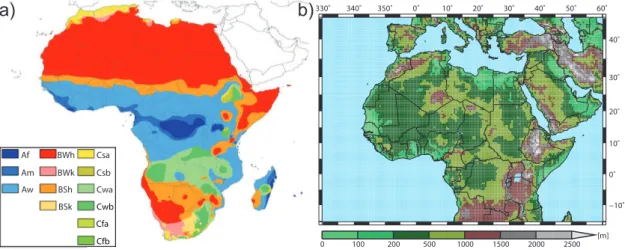
Fig. 2.1: (a) Köppen climate classification of Africa (Peel et al. 2007, their Fig. 4). A: tropical, B: arid, C: temperate climate; f: rainforest, m: monsoon, w: savannah; W: desert, S: steppe; h: hot, k:
cold; s: dry summer, w: dry winter, f: without dry season; a: hot summer, b: warm summer. (b) Orography of Africa as used by REMO (cp.Paeth et al. 2009) including national boundaries and major lakes.
According to the Köppen climate classification, Africa is dominated by three main climate types, namely an arid, a tropical, and a temperate climate (Peel et al. 2007). Due to the subtropical high pressure belts in the Northern and Southern Hemisphere more than half of the continent (i.e. in the area and vicinity of the Sahara and Namib Deserts), is characterised by arid conditions (see Fig.2.1a). In contrast, the central part of Africa exhibits a semi-humid or humid tropical climate. A temperate climate is partially found in southern Africa and to some extend in the Ethiopian Highlands. Parts of the north of Africa have a Mediterranean climate.
Individual rainfall-producing weather systems account for the variability in the cli- matological precipitation amount in tropical Africa (e.g.,Le Barbé and Lebel 1997;Shin- oda et al. 1999;Le Barbé et al. 2002). During the rainy season there is a high frequency of rainfall events due to the short duration of the water vapour discharge-loading cycle (e.g., Peters and Tetzlaff 1988). Several types of precipitation systems were found to cause rainfall over tropical Africa (cf.Fink et al. 2006 and references therein). These comprise, for example, organised mesoscale convective systems, monsoon rains, and local showers or instability storms.
Due to the close relation of malaria with climate and weather conditions (cp. Sec.2.6.1) the following sections provide further information on the climate of West Africa and the Greater Horn of Africa (see Fig.G.3).
2.1.1 The climate of West Africa
The climate of West Africa transitions between an equatorial tropical climate in the south and a warm desert climate in the north. During boreal summer the climate is largely controlled by the West African monsoon circulation, which produces the bulk of annual precipitation. During boreal winter the dry season is characterised by dry and dusty northeasterly Harmattan winds that originate from the Sahara Desert (e.g.,Buckle 1996).
The climate of West Africa is affected by both cool and humid monsoon air masses as well as hot and dry Saharan air masses. The InterTropical Front (ITF), also termed monsoon trough in the literature, defines the border between these two air masses (e.g., Hamilton and Archbold 1945; see Fig.2.2). In contrast, the InterTropical Convergence Zone (ITCZ) is defined by the maximum water vapour convergence in a tropospheric column (Fink 2006). The ITCZ is generally located between 6◦ and 10◦ latitude south of the ITF and is associated with strong precipitation amounts (e.g.,Ermert and Brücher 2008).
Due to the wedge-shaped penetration of the monsoon air under the Saharan air mass, the atmospheric layering becomes baroclinic (e.g., Fig. 3 inPytharoulis and Thorncroft 1999). The result of this temperature contrast is a westward thermal wind, the so-called African Easterly Jet (AEJ), that maximises at a height of about 650 hPa where the north- south temperature gradient reverses (e.g.,Burpee 1972, his Fig. 2). The AEJ maximum is located between about 10-15◦N (e.g.,Parker et al. 2005) at the time of the northernmost position of the ITF at about 20◦N during August (e.g.,Flohn 1965).
The baroclinic and barotropic instability of the AEJ is leading to westward- propagating low-level African Easterly Waves (AEWs; e.g., Thorncroft and Hoskins 1994), which are the dominant synoptic-scale features of the West African monsoon during boreal summer (e.g., Carlson 1969b,a). There is an interaction of AEWs with rainfall bearing systems (e.g., Reed et al. 1977; Payne and McGarry 1977). AEWs primarily trigger cloud clusters ahead of an AEW trough and west of the Greenwich meridian (Fink and Reiner 2003).
2.1 THE CLIMATE OFAFRICA 7 The atmospheric conditions above West Africa are continuously changing through- out the year. Between November and March during the dry season, the Sahelian and Sudanian zone are located north of the ITF (Fig.2.2). The northeasterly trade winds, known as the Harmattan, prevail. The Harmattan blows across the Sahara Desert and is therefore dry and dusty (e.g.,Hamilton and Archbold 1945). During the first part of the dry season between November and January, the Harmattan airflow is cool, causing the cool dry season. From February to May the Harmattan air mass is increasingly heated due to the higher sun angles, a longer length of day, and the dominance of sensible heat fluxes in the heat budget of the near surface layer. During this hot dry season the highest annual temperatures are observed, with maximum temperatures well above 40◦C. Strong daytime insolation as well as clear and dry nights lead to a large mean daily temperature range.
During boreal spring the increasing solar radiation over the Sahel and Sahara re- gions causes a strengthening and northward progression of the continental heat low (cp.Pedgley 1972). In its wake, the relatively cool, moist, and convectively unstable monsoon air penetrates farther into the continent (cp.Thorncroft et al. 2003; their Fig. 6).
During the pre-onset of the monsoon the depth of the monsoon layer increases and short- term northward excursions of the ITCZ cause first substantial rainfalls along the Guinean coast. Farther north in the Sudanian zone the start of the rainy season is delayed until May or June (cp.Le Barbé et al. 2002). At the end of June, during the main onset of the monsoon system, the ITCZ abruptly jumps from 5◦N to approximately 10◦N, resulting in abundant rainfall and cloudier conditions in the Sahel (cp.Sultan et al. 2003;Sultan and Janicot 2003). During this time, the coast is affected by the ‘little dry season’, which is directly related to coastal upwelling, a colder Sea-Surface Temperature (SST), and the resulting drop of rainfall (Vollmert et al. 2003). The swift retreat of the monsoon system and the ITCZ toward the equator from September to November causes a second and less intense rainy season in the south (cp.Omotosho 1985). By the end of November, the ITCZ is situated far from the coast and the dry season is again set in place over West Africa (e.g.,Le Barbé et al. 2002).
2.1.2 The climate of the Greater Horn of Africa
The dynamics and variability of the climate of the Greater Horn of Africa are quite com- plex. The large-scale circulation is superimposed upon regional factors associated with lakes, orography, and maritime influences (see Fig.2.1b). Various spatial and tempo- ral processes determine the geographical distribution of diverse climatic zones. Climate ranges from desert to tropical rain forest with a transition over relative small distances (cp. Fig.2.1a). Areas with a uni-, bi-, or trimodal annual rainfall are located within distances of markedly less than 100 km (e.g.,Davies et al. 1985, their Figs. 3 & 4). De- spite this diversity, large parts of East Africa, such as the equatorial zone, experience a fairly similar interannual variability of precipitation, primarily linked to large-scale at- mospheric and oceanic changes (e.g.,Nicholson 1996; see Sec.2.1.3). Due to the great
latitudinal extension of the Greater Horn of Africa, the following analysis will separate between climate conditions of Equatorial East Africa (EEA; southern Ethiopia, Kenya, western Somalia, Uganda, Rwanda, Burundi, and Tanzania) and Northeast Africa (NeA;
eastern Sudan, Eritrea, Ethiopia, and Djibouti; see Figs.G.1&G.3).
The climate of the Greater Horn of Africa is predominantly affected by three main air streams and three convergence zones (see Fig.2.2). During high and low sun sea- sons this area is affected by a southeastern and northeastern monsoon flow, respectively.
These airflows are representing in part the western edge of the Asian monsoon, are par- allel to the coast, and are strongly meridional. They do not represent a classical monsoon which moves moist air on- and dry air offshore (Buckle 1996). By contrast to the West African monsoon, both the southeasterly and the northeasterly monsoon flow are asso- ciated with relatively dry conditions. The third stream represents a west, southwesterly flow that transports humid, convergent, and thermally unstable Congo air and is associ- ated with rainfall. The air streams are separated by the monsoon trough and the Congo Air Boundary. A third convergence zone in the middle troposphere borders the dry and stable northerly air from the Sahara and the more humid southerly air mass (Nicholson 1996).
Fig. 2.2: Schematic pattern of general winds (arrows), pressure systems (solid lines), convergence zones (dashed lines), as well as the monsoon trough (dotted lines) for (a) the January and (b) the July/August circulation over Africa (afterNicholson 1996).
EEA is affected by two distinct equinoctial rainy seasons. Main rain-bearing sys- tems commonly occur during transition seasons, when the meridional flow is interrupted between March and May as well as between October and December (seeGatebe et al.
1999, their Tab. 1). Semiannual precipitation is therefore basically related to the migra- tion of the ITCZ (e.g., Behera et al. 2005) corresponding to the movement of the belt of maximum solar insolation (Marchant et al. 2006). During these periods the flow is often onshore and is forced to ascend by topography and coastal friction (Nicholson 1996). Maximum rainfall generally lags the position of the overhead sun by approxi- mately one month (Black et al. 2003). Double peaks in rainfall are usually termed long and short rains (e.g., Hastenrath et al. 1993). Between March and May the northward passage of the ITCZ causes the more abundant long rains. During boreal summer the
2.1 THE CLIMATE OFAFRICA 9 persistent southerly monsoonal flow leads to active coastal upwelling that produces cold SSTs along the eastern coast of the Greater Horn of Africa (seeBehera et al. 2005, their Fig. 1). This fact as well as the swift retreat of the monsoon system in boreal autumn (see Leroux 1983) explains the shorter duration of heavy rainfall and lower intensity of the short rains in October and November. Although, most precipitation is associated with the long rains, the short rains experience a larger degree of interannual variability (Has- tenrath et al. 1993). An accurate prediction of the strength of short rains is therefore of considerable importance for agriculture and epidemic diseases like malaria (Clark et al.
2003). Outside of the transition seasons, rainfall is mostly linked to the humid Congo air mass and occurs especially over the Western Rift Valley (Fig.G.1)1. A third rainfall sea- son is limited to parts of western Kenya and Uganda, is most pronounced in July-August and contributes significantly to annual precipitation (Davies et al. 1985).
NeA is also affected by the migration of the monsoon system causing uni- and bi- modal rainfall patterns. During the dry season from October to December/January (lo- cally known as the Bega), rainfall is restricted to tropical-extratropical interactions and to occasional developments of the Red Sea Convergence Zone at the coastal plains and eastern escarpment of Eritrea (Seleshi and Zanke 2004). Between February and April converging northeast and southeast winds produce a brief period of rainfall, known as the Belg rains (e.g., Diro et al. 2009). During this time, precipitation falls in southern, central, and eastern parts of Ethiopia. In May, rainfall decreases due to the strengthening of the Egyptian High (Conway 2000). The bulk of precipitation (65-95% of total annual rainfall) in NeA falls in the so-called Kiremt season between June and September, when the ITCZ moves over the area (Segele and Lamb 2005; see Fig.2.2). The southwesterly air stream transports moisture from the Atlantic and Indian Ocean into the region (e.g., Diro et al. 2009). The mean airflow as well as orographic lifting produce abundant pre- cipitation in the western parts of the Ethiopian Highlands (Segele and Lamb 2005, their Fig. 1). Precipitation decreases to the north toward Eritrea to about 600 mm of rain in June-August mainly due to weaker upper level forcings (Segele et al. 2008). In general, Kiremt rainfall is influenced by the Arabian and Sudan thermal lows, which determine the position of the ITCZ, as well as upper level features such as the AEJ and TEJ. More- over, the strength of Sankt Helena and Mascarene Highs as well as the low-level Somali jet are affecting the southwesterly flow (Seleshi and Zanke 2004;Diro et al. 2009).
Some local effects play a role in the distribution of rainfall and temperature in East Africa. For example, elevation differences and other topographical characteris- tics greatly influence the climate of East Africa. The highlands of the Western Rift Valley block the moist and unstable westerly airflow from the Atlantic. Likewise, the Ethiopian Highlands provide leeward rain shadows leading to a complex pattern of rain- fall and aridity along the Great Rift Valley, down to the Afar Depression, as well as in the Ogaden (cp.Nicholson 1996; Conway 2000). Highland territories exhibit zones with relatively low temperatures. During the wet season, temperature decreases by about
1See App.Gfor the geographical positions of various territories, highlands, mountains, lakes, as well as towns.
5.3◦C per 1000 m of elevation in Ethiopia for example. Mean annual temperatures in the Ethiopian Woina Dega (Dega) climate zone are 16-20◦C at an altitude between 1800 and 2400 m and only 6-16◦C above 2400 m (Conway 2000). In northern Kenya, divergence in the airflow is associated with the low-level Lake Turkana Jet, which is channelled by the Ethiopian and East African highlands (Kinuthia 1992;Camberlin 1997, his Fig. 3).
Large water bodies significantly alter the convective activity (cp.Ogallo 1989). The rain- fall over Lake Victoria, for example, is dramatically enhanced by a nocturnal lake-breeze circulation (Ba and Nicholson 1998). In contrast, the upwelling of cold water along the Somali coast suppresses moist convection along the coast (cp.Halpern and Woiceshyn 1999;Hodges 1998).
2.1.3 Interannual variability of precipitation
Africa is known for its variable climate, often exceeding the range of variation of many other places on Earth. In Africa, climate variability is mainly manifested as changes in rainfall. One striking feature are the overall drier conditions in the Sahel since the 1970s, even though the Central Sahel recently exhibits an upward trend (e.g.,Nicholson 2005;
Ali and Lebel 2009; Lebel and Ali 2009). In Africa, rainfall distributions in space and time have been studied extensively due to their importance for economy, agriculture, and epidemic diseases. Anomalously low or high rainfall amounts can give rise to drought or floods, respectively, both with disastrous economic and humanitarian consequences (Washington et al. 2006). In November-December 1997, for example, unusual high rainfall gave rise to a major malaria epidemic in northeastern Kenya (Brown et al. 1998).
Oceans markedly influence the characteristics and circulation of the atmosphere.
The atmospheric boundary layer of the tropical Atlantic, for example, is enriched by moisture from the Atlantic Ocean, feeding the West African summer monsoon (cp.Cadet and Nnoli 1987). The temperature contrast between oceans and adjacent continental land masses determines the flow of air (cp.Haarsma et al. 2005). Cold (warm) SSTs suppress (enhance) the formation of deep convection and hence rainfall (e.g.,Vollmert et al. 2003).
Due to the migration of atmospheric features, the impact of an SST anomaly depends on season. SST anomalies may enhance rainfall in one season, but reduce it in another (cp.Balas et al. 2007). On a larger scale, oceans influence the generation of the Walker circulation. This equatorial feature is able to link local processes to the large-scale.
Ascending and descending branches of the Walker cell directly influence the thermal static stability of the troposphere. For these reasons, natural or anthropogenic changes in oceans have a strong influence on Earth’s climate.
West Africa
The Sahel has attracted special interest because of its drought conditions in the 1970s and 1980s. Research has moved steadily away from explanations for rainfall variations in this region as primarily due to land use changes and more towards explanations based
2.1 THE CLIMATE OFAFRICA 11 on SST changes (Christensen et al. 2007a). On interannual and interdecadal time scales Sahel rainfall is largely determined by fluctuations in SSTs. Atmospheric simulations using General Circulation Models (GCMs) show that the north-south interhemispheric SST gradient is most important. Colder oceans in the Northern Hemisphere and warmer low-latitude SSTs around Africa weaken the continental convergence associated with the summer monsoon (cp.Giannini et al. 2003;Hoerling et al. 2006). In particular, cold (warm) SSTs in the Atlantic Ocean in the region south of West Africa favour a strong (weak) monsoon circulation and lead to wet (dry) conditions in the Sahel (cp.Lamb 1978;Eltahir and Gong 1996). Warm SSTs in the equatorial Atlantic favour an anoma- lously southerly ITCZ location (cp.Balas et al. 2007) that leads to increased precipita- tion along the Guinean coast (cp.Ruiz-Barradas et al. 2000). Bader and Latif (2003) suggested that the warming trend in the Indian Ocean played a crucial role for the dry- ing trend over the Sahel (see alsoPalmer 1986;Giannini et al. 2003;Lu and Delworth 2005;Hoerling et al. 2006). A warm Indian Ocean enhances convection over the tropi- cal Indian Ocean resulting in upper tropospheric divergence. This divergence induces an unusual east-west circulation and upper level convergence over West Africa, which ulti- mately suppresses rainfall. In addition,Rowell(2003) concluded that a warmer Mediter- ranean Sea tends to moisten the Sahel. In such a situation, a higher moisture content of the lower troposphere, which is advected southward across the eastern Sahara, produces additional precipitation. Finally, there seems to be a Pacific-Sahel teleconnection (e.g., Janicot et al. 1996). A warm El Niño/Southern Oscillation (ENSO) might generate inter- acting stationary equatorial waves enhancing large-scale subsidence over the Sahel (see Rowell 2001). Janicot et al.(2001) proposed that moisture advection over West Africa is reduced during El Niño years through induced changes in pressure gradients.
Atmospheric conditions are also markedly influenced by surface conditions of land masses. Vegetation partly determines the surface albedo, recycles precipitable water via transpiration, and affects various other processes (seeChristensen et al. 2007a, their Box 11.4). Charney’s hypothesis, for example, points to a positive albedo-precipitation feedback (Charney 1975). An increase in surface albedo due to an anthropogenic reduc- tion in vegetation could cause a decrease in precipitation that, in turn, would lead to a decrease in vegetation cover and thus a further enhancement of albedo. Indeed,Giannini et al. (2003) argued that the response of the West African summer monsoon to oceanic forcing is amplified by land-atmosphere interactions (cp. also Taylor et al. 2002). The variance of rainfall in the GCM is weaker in absence of a feedback between the atmo- spheric circulation and land surface processes. However, the sign of rainfall anomalies in the Sahel is still determined by SST variability.
Recent research indicated that changes in SST have probably the dominant influence on Sahel rainfall (cf.Hegerl et al. 2007;Christensen et al. 2007a). A spatially varying, anthropogenic sulphate aerosol forcing is found to provide an important feedback on the cooling at high latitudes and changes in the interhemispheric SST gradients result in a southward shift of the ITCZ (Williams et al. 2001;Biasutti and Giannini 2006). Aerosols seem to have a key role in the determination of lifetime and albedo of clouds (Rotstayn
and Lohmann 2002). Effects of clouds on Sahel rainfall were further demonstrated by Haarsma et al. (2005). Their climate scenarios led to an increase in low-level clouds over oceans contributing to less warming over oceans than over the Sahara. This again induces a stronger summer monsoon and therefore a wetter Sahel.
Greater Horn of Africa
A strong interannual variability of rainfall in EEA has been found for the short rains and is mainly influenced by the Indian Ocean. In Kenya and Tanzania, for example, the October-November rainfall is highly correlated to annual rainfall despite its lower amounts (Nicholson 1996).
EEA rainfall in boreal autumn seems to depend on the strength of a Walker cell.
In the interval between the northeast and southwest monsoons in boreal autumn, a closed zonal circulation materialises above the Indian Ocean equator (Hastenrath 2000;
cp. Fig.2.3a). This circulation accelerates equatorial surface westerlies driving the oceanic Eastward Equatorial Jet (cp.Wyrtki 1973) in the upper part of the Indian Ocean (Luyten et al. 1980; Hastenrath et al. 1993). The formation of the jet in the tropical ocean is accompanied by a flattening of the thermocline at its western origin (Wyrtki 1973). The regime of a weak atmospheric zonal circulation entails slow westerlies, a de- creased subsidence, and abundant rainfall in EEA (Hastenrath 2001; see alsoJury et al.
2002). It also seems to be found preferably under El Niño conditions (cp.Hastenrath 2000).
More recently, the atmospheric fluctuation described above has been associated with the so-called Indian Ocean Dipole (IOD; first described bySaji et al. 1999). IOD events show large-scale SST anomalies producing enhanced EEA rainfall. SST anomalies in the Indian Ocean had traditionally been viewed as an outcome of the ENSO system (e.g., Nicholson and Nyenzi 1990; Nicholson 1996) that is forced under El Niño and suppressed under La Niña conditions, but there is increasing evidence that it is a sepa- rate and distinct phenomenon (Marchant et al. 2006). Behera et al. (2005) showed that the IOD influence on short rains in EEA is overwhelming as compared to that of ENSO (see alsoSaji and Yamagata 2003a, their Fig. 1). In particular, 1961 – the second largest IOD event of the 20th century – was not an El Niño year (e.g.,Black et al. 2003). More- over,Saji and Yamagata(2003b) found that the strength of ENSO events might actually depend on the IOD mode. They noted that ENSO events co-occurring with IOD events are much stronger compared to unrelated events. However, other studies concluded that in some occasions ENSO can force IOD events (e.g., Black et al. 2003; Clark et al.
2003).
During boreal autumn a positive dipole mode of the IOD is associated with a distinct dipole-like SST pattern in the tropical Indian Ocean (e.g.,Saji and Yamagata 2003b, their Fig. 2). Such events show cool (warm) SST anomalies in the east (west) Indian Ocean (e.g., Webster et al. 1999; Fig.2.3b). The troposphere above the Indian Ocean shows a strong variability during a positive IOD event, which is characterised by following
2.1 THE CLIMATE OFAFRICA 13
Fig. 2.3: (a) Illustration of the usual Walker circulation along the equator (after Nicholson 1996).
(b) Schematic of the IOD event in 1997 (fromWebster et al. 1999). A cool (warm) SST anomaly occurred in the eastern (western) Indian Ocean in the second half of 1997. In autumn 1997, the heating anomaly off the East African coast changed the usually weak climatological equatorial westerlies to surface easterlies (left panel). The SST anomalies came along with anomalies in the sea surface height, which was decreased (increased) in the eastern (western) basin of the Indian Ocean (right panel).
structures: (i) Walker cell anomaly over the equator; (ii) deep modulation of monsoon westerlies; and (iii) an anomalous Hadley cell over the Bay of Bengal (Saji and Yama- gata 2003a). A positive dipole mode weakens the westerly flow that normally transports moisture away from the African continent out over the Indian Ocean (Black et al. 2003;
Fig.2.3). The normal convection patterns situated over the eastern Indian Ocean warm pool are shifted westward and bring abundant short rains over EEA as well as drought conditions causing forest fires over the Indonesian region (Marchant et al. 2006). Posi- tive IOD events therefore result in significant rain variability in surrounding land masses (see also Fig.2.3) and unusual high (low) temperatures over countries west (east) of the Indian Ocean.
The climate of NeA also exhibits a large interannual variability. Much like the Sa- hel, droughts in the 1970s and 1980s in Ethiopia resulted in low agricultural production and affected millions of people (e.g., Seleshi and Zanke 2004). Atmospheric features significantly influencing rainfall of NeA include ENSO, SSTs in the Indian Ocean, and pressure systems, which steer moisture advection.
A large-scale teleconnection with ENSO markedly influences Kiremt (June- September) precipitation in NeA. It was found that El Niño years are typically associated with lower rainfall amounts and drought years. A late onset and short Kiremt season is likely to be connected with El Niño conditions. In contrast, La Niña conditions usually lead to higher precipitation quantities (e.g.,Beltrando and Camberlin 1993;Segele and Lamb 2003, 2005;Seleshi and Zanke 2004;Block and Rajagopalan 2007;Korecha and
Barnston 2007; Segele et al. 2008). As previously noted, ENSO events seem to alter zonal Walker-type circulations. Westerly (easterly) anomalies in lower (upper) levels cause an increased moisture flow towards the area and hence abundant summer rainfall years (Camberlin 1995). A different response was detected for the Belg season, when El Niño can produce excess rainfall (cp.Diro et al. 2009).
Interannual Kiremt rainfall variability is also linked to pressure patterns. Anoma- lously low pressure in India triggers a west-east pressure gradient near the equator inten- sifying the monsoon flow over the Indian Ocean and Africa. An enhanced Indian mon- soon leads to a stronger moisture advection from the Congo Basin toward NeA (Cam- berlin 1995,1997). Moreover, an intensification of pressure over the Gulf of Guinea in the Atlantic enhances the westerly/southwesterly monsoon flow across the continent and produces wetter conditions over the Horn of Africa (Segele and Lamb 2005;Segele et al.
2008).
Rainfall in NeA is also correlated with SSTs near Africa. Warm SSTs in the west- ern Indian Ocean and the Arabian Sea are associated with a delayed Kiremt cessation and hence prolonged rainfall (Segele and Lamb 2003, 2005). It is interesting to note that Kiremt rainfall does not seem to depend on IOD conditions (see above). Saji and Yamagata(2003a) found that in the southern part of Ethiopia (3-7◦N, 32-46◦E) Kiremt rainfall is significantly correlated with ENSO but not with the IOD.Segele et al.(2008) established that warm (cool) SSTs in the southern Indian Ocean leads to reduced (en- hanced) Ethiopian monsoon rainfall. They argued that a warm (cool) southern Indian Ocean weakens (intensifies) the Mascarene high and hence the flow. Furthermore, the number of tropical depressions over the southwest Indian Ocean predominantly affects precipitation of the Belg season.Shanko and Camberlin(1998) showed that a high (low) number of tropical depressions is negatively (positively) correlated with Belg rainfall.
During boreal winter the presence of tropical depressions reduces the moisture advec- tion toward Ethiopia due to an enhanced flow into the systems.
2.2 IPCC SRES scenarios
Greenhouse gases reduce the loss of heat of the Earth’s atmosphere. GHGs include carbon dioxide (CO2), nitrous oxide (N2O), methane (CH4), sulphur oxides (SOx), and various other gases such as halocarbons. Increased anthropogenic GHG emissions since the industrial revolution have changed the natural balance and led to a rise of global surface temperatures of 0.74◦C between 1906 and 2005 (Trenberth et al. 2007). For this reason, impressions of the future evolution of GHG concentrations are essential for Earth’s climate projections. Already at the start of the 1990s, the IPCC developed six alternative scenarios (Houghton et al. 1992). These scenarios were finally superseded by the IPCC Special Report on Emissions Scenarios (SRES; seeNaki´cenovi´c et al. 2000).
Some basic information with an emphasis on A1B and B1 climate scenarios is presented below.
2.2 IPCC SRES SCENARIOS 15
a) b)
A1T A1B A1FI
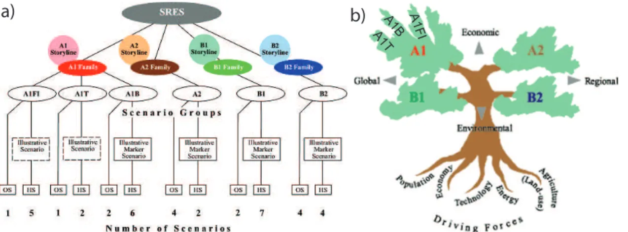
Fig. 2.4: Schematic illustration of SRES scenarios (after Naki´cenovi´c et al. 2000). In (a) HS denotes scenarios with ‘harmonised’ assumptions on global population, gross world product, and finite energy, whereas OS scenarios explore uncertainties in driving forces beyond those of harmonised scenarios. Under (b) the four scenario ‘families’ are depicted as branches of a tree. Further details see text.
Driving forces of GHGs are mainly the demographic and socio-economic develop- ment as well as changes in technology and the environment. Naki´cenovi´c et al.(2000) presented four different narrative storylines (the so-called ‘families’ are A1, A2, B1, and B2) that estimate future progression of emissions. Six scenario groups are drawn from the four families (cp. Fig.2.4). One group each in A2, B1, and B2 as well as three groups within A1 characterised by different energy technology developments: A1FI describes a fossil fuel (including coal, oil, and gas) intensive, A1B follows a balanced energy supply mix, and A1T is a predominantly non-fossil fuel scenario.
The level of economic activity by 2100 ranges between ten and 26 times the gross world product values of 2000. By 2100 the A1 scenario family represents the upper bound of the gross domestic product, whereas the B1 scenario family is intermediary.
Alternative pathways are explored to describe a convergent world. The A1 scenario family is characterised by capacity building, and increased cultural as well as social interactions. Alternatively, rapid changes in economic structures towards a service and information economy take place under B1.
Technology change will strongly impact future GHG emissions of the 21st century.
B1 and to some extent also A1B follow a trend toward an increase of renewable and nuclear energies in the long term. A1 and B1 scenarios expect significant innovations in energy technologies and drastic reductions in costs for solar, wind, and other renewable energies. Clean and resource-efficient technologies are introduced in the B1 scenario, whereas A1B has a balanced emphasis on all energy sources.
The population growth until 2050 as well as dietary changes result in a global ex- pansion of grassland and pasture at the expense of forest area under the A1 storyline.
An increased productivity largely compensates the growing food demand under B1. By 2100, B1 and B2 scenario families include a considerable ‘greening’ of the planet, due