TIRF-anisotropy microscopy: homo-FRET and single molecule measurements

Dissertation

zur Erlangung des akademischen Grades eines Doktors der Naturwissenschaften

TIRF-anisotropy microscopy:

homo-FRET and single molecule measurements

vorgelegt von

M´ arton Gell´ eri

September 2013

Erstgutachter: Prof. Dr. Philippe Bastiaens

Zweitgutachter: Prof. Dr. Roland Winter

Erkl¨ arung/Declaration

Die vorliegende Arbeit wurde in der Zeit von November 2008 bis September 2013 am Max-Planck-Institut f¨ ur molekulare Physiologie in Dortmund unter der Anleitung von Prof. Dr. Philippe I. H. Bastiaens durchgefuhrt.

Hiermit versichere ich an Eides statt, dass ich die vorliegende Arbeit selbst¨ andig und nur mit den angegebenen Hilfsmitteln angefertigt habe.

The present work was accomplished from November 2008 to September 2013 at Max-Planck-Institute for molecular physiology in Dortmund under the guidance of Prof. Dr. Philippe I. H. Bastiaens.

I hereby declare that I performed the work presented independently and did not use any other but the indicated aids.

Dortmund, September 2013

M´ arton Gell´ eri

Abstract

Optical microscopy is limited by diffraction to a resolution of approximately half the wavelength of the light used. Recent fluorescence microscopy meth- ods increase the optical resolution by localizing single molecules with a pre- cision exceeding the diffraction limit. Sequential imaging of all fluorescent proteins in such an approach allows the reconstruction of a super-resolution image. The gain in resolution can be used to investigate the organization of proteins within cells on a sub-micrometer scale.

In this thesis, we combined localization microscopy with polarization mea- surements and total internal reflection fluorescence (TIRF) microscopy to investigate the spatial organization of plasma membrane proteins. The de- veloped microscope was used in ensemble measurements to probe protein organization at a nanometer scale via F¨ orster Resonance Energy Transfer (FRET) and to investigate molecular orientations on a single molecule level.

TIRF microscopy was combined with fluorescence anisotropy measure- ments to investigate the spatial organization of the small GTPase Ras and its active mutants. In ensemble measurements the presence of FRET leads to depolarization of the emitted fluorescence signal, and probing distances on the nanometer scale is possible. It was shown that anisotropy measurements with conventional wide field excitation as well as with TIRF excitation are hampered by high noise levels making it difficult to draw clear conclusions.

Anisotropy measurements were also carried out on a single molecule level. On a single molecule level polarization becomes a measure of the two-dimensional orientation of molecules. Stepwise bleaching experiments showed that polarization measurements allow the detection of homo-FRET on a single molecule level.

Photoactivated localization microscopy (PALM) was combined with ori- entation measurements. The effect of photoselection by the excitation light on a common PALM sample was investigated by rotating the polarization of the excitation light and measuring the distribution of molecular orientations.

It was shown that the polarization of the excitation light can bias single mo-

lecule measurements. For a non-random distribution of the fluorophores this

bias can result in misleading conclusions.

Zusammenfassung

Lichtmikroskopie wird durch die Beugung von Licht auf eine Aufl¨ osung von etwa der halben Wellenl¨ ange des Lichtes begrenzt. Neuere Methoden der Fluoreszenzmikroskopie umgehen diese Beugungsgrenze, indem die Position einzelner fluoreszierender Molek¨ ule mit einer Genauigkeit bestimmt wird, die weit ¨ uber der Aufl¨ osungsgrenze konventioneller Lichtmikroskopie liegt.

Um diese Aufl¨ osung zu erreichen, wird eine Bildfolge von fluoreszierenden Molek¨ ulen aufgenommen, die zu einem hochaufl¨ osenden Mikroskopiebild re- konstruiert wird. Die erh¨ ohte Aufl¨ osung kann dann benutzt werden um die r¨ aumliche Verteilung von Proteinen in Zellen auf einer Submikrometerskala zu untersuchen.

Um die r¨ aumliche Organisation von Plasmamembranproteinen zu unter- suchen, wurden in der vorliegenden Arbeit Lokalisationsmikroskopie mit Po- larisationsmessungen und interner Totalreflexionsmikroskopie (englisch: to- tal internal reflection fluorescence microscopy, TIRF microscopy) kombiniert.

Das entwickelte Mikroskop wurde sowohl in Ensemble-Messungen eingesetzt um die Proteinorganisation mittels F¨ orster Resonanz Energietransfer (FRET) auf der Nanometerebene zu untersuchen, als auch in Einzelmolek¨ ulmessungen um molekulare Orientierungen zu betrachten.

TIRF Mikroskopie wurde mit Fluoreszenzanisotropiemessungen kombi- niert um die r¨ aumliche Verteilung der kleinen GTPase Ras und ihren ak- tiven Mutanten zu untersuchen. In Ensemble-Messungen f¨ uhrt FRET zu einer Depolarisation des emittierten Fluoreszenzsignals, so dass Distanzen auf der Nanometerskala untersucht werden k¨ onnen. Es konnte gezeigt wer- den, dass Anisotropiemessungen sowohl in konventioneller Weitfeldanregung als auch in TIRF-Anregung durch den hohen Hintergrund beeintr¨ achtigt und dadurch R¨ uckschl¨ usse auf die Proteinorganisation erschwert werden.

Anisotropiemessungen wurden auch auf Einzelmolek¨ ulebene durchgef¨ uhrt.

Auf Einzelmolek¨ ulebene entspricht die Messung der Polarisation einer Mes-

sung der zweidimensionalen Orientierung der Molek¨ ule. Stufenweises Ble-

ichen von Molek¨ ulen zeigte, dass Polarisationsmessungen die Detektion von

homo-FRET in Einzelmolek¨ ulmessungen erlauben.

Photoaktivierte Lokalisationsmikroskopie (PALM) wurde mit Polarisa-

tionsessungen kombiniert. Der Einfluss der Photoselektion wurde f¨ ur eine

typische Probe untersucht, indem die Polarisation des Anregungslichtes ge-

dreht wurde und die Verteilung der Orientierungen der Molek¨ ule bestimmt

wurde. Es konnte gezeigt werden, dass die Polarisation des Anregungslichtes

einen Einfluss auf Einzelmolek¨ ulmessungen hat. F¨ ur eine nichtzuf¨ allige Ver-

teilung der Fluorophore kann dieser Einfluss zu falschen R¨ uckschl¨ ussen f¨ uhren.

expect, even when you take into account Hofstadter’s Law

Douglas R. Hofstadter

Abstract iii

Zusammenfassung v

1 Introduction 1

2 Theoretical background 5

2.1 Photophysics of fluorescent probes . . . . 6

2.1.1 Fluorescence . . . . 6

2.1.2 Fluorescence anisotropy . . . . 8

2.1.3 F¨ orster resonance energy transfer . . . . 13

2.2 Microscopy . . . . 17

2.2.1 Resolution limit . . . . 17

2.2.2 Localization based super-resolution techniques . . . . . 20

2.2.3 Total internal reflection . . . . 24

2.2.4 Fluorescence anisotropy microscopy . . . . 27

2.2.5 TIRF anisotropy . . . . 31

2.3 Review of fluorescence anisotropy imaging literature . . . . 33

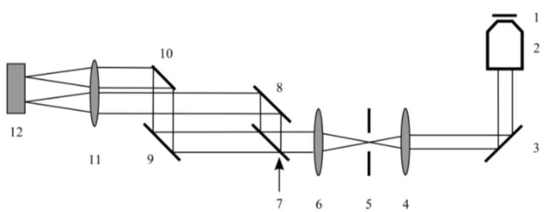
3 Experimental realization of TIRF-anisotropy 35 3.1 Excitation path . . . . 36

3.2 Emission path . . . . 38

3.2.1 Modifications to the setup in super-resolution microscopy 40 3.3 Measurement of the G-factor . . . . 41

3.4 EM-CCD . . . . 43

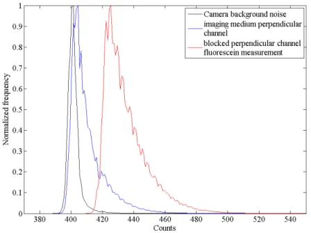
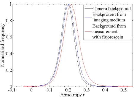
3.4.1 Background correction . . . . 45

3.5 Image registration of polarization data . . . . 49

4 Ensemble measurements by TIRF-anisotropy 51 4.1 Materials and methods . . . . 52

4.1.1 Acquisition of microscopy data . . . . 52

4.1.2 Sample preparation . . . . 52

4.1.3 Data analysis . . . . 53

4.2 Validation measurements . . . . 53

4.2.1 Measurement of anisotropy in wide field microscopy . . 53

4.2.2 Measurement of cytosolic Citrine . . . . 55

4.3 Application to biology . . . . 58

4.3.1 Spatial organization of HRas and KRas . . . . 60

4.4 Conclusion . . . . 62

5 Single molecule measurements by polarized TIRF 71 5.1 Materials and Methods . . . . 72

5.1.1 Acquisition of microscopy data . . . . 72

5.1.2 Sample preparation . . . . 72

5.1.3 Data analysis . . . . 73

5.2 Validation measurements . . . . 73

5.2.1 Measurement of orientation of Pt-Complex fibers . . . 74

5.3 Orientation measurement of single molecules . . . . 78

5.4 Conclusion . . . . 83

6 Application to super-resolution by localization microscopy 85 6.1 Materials and Methods . . . . 86

6.1.1 Acquisition of microscopy data . . . . 86

6.1.2 Sample preparation . . . . 87

6.1.3 Data analysis . . . . 88

6.2 Photoactivated localization microscopy . . . . 89

6.3 Polarized excitation . . . . 90

6.3.1 Standard PALM measurements . . . . 92

6.3.2 Photobleaching of one polarization component . . . . . 93

6.4 Polarized emission . . . . 93 6.4.1 Orientation measurements in photoactivated localiza-

tion microscopy . . . . 95 6.5 Conclusion . . . . 99

7 Conclusion and outlook 103

7.1 Conclusion . . . 103 7.2 Outlook . . . 105

References 109

Acknowledgments 125

Introduction

Multicellular systems form complex structures of highly differentiated cells.

The cells drive a highly complex system of dynamic processes and communi- cate with their neighboring cells, even without direct contact. In both cases the information generated within the cells has to pass the cell membrane.

The information can be an electrical or a metabolic signal, where the latter requires receptor molecules in the cell membrane. At the same time a single cell itself is a highly complex system. Driven by a dynamic network of in- teracting proteins it forms temporal and spatial patterns that are important for cell signaling.

The function of these receptors and proteins can be investigated by ap-

plying biochemical or physiological methods. However, to investigate their

spatial organization, imaging techniques such as microscopy have to be ap-

plied. Microscopy enables the user to observe structures and processes in

cells on a sub-micrometer scale. A commonly used technique in the bio-

logical sciences is fluorescence microscopy. In fluorescence microscopy, the

molecules of interest are tagged with fluorescent markers. These markers

emit light upon excitation and can be detected within the cell. However,

any optical microscope is fundamentally limited by the diffraction of light to

a resolution of roughly 200 nm laterally and 600 nm axially. Nevertheless,

the specific tagging of proteins allows the detection and imaging on a single

molecule level, making it possible to record the movement of single molecules

in living cells. A wide variety of available microscopy techniques allows for addressing specific biological problems, but at the same time makes it nec- essary to thoroughly think about the imaging methods and techniques used to determine the measurement parameters of interest.

Investigation of the nanoscale organization of plasma membrane proteins requires a microscope capable of probing distances well below the diffraction limit of light. This can be achieved using two different techniques: FRET microscopy, which uses the dipole-dipole coupling of two molecules in reso- nance to measure distances in the range of 5 to 10 nm, and single molecule localization microscopy, which accesses spatial scales of around 20 nm. These microscope techniques, being complementary on the length scale, are both fluorescence microscopy methods, thus allowing the specific tagging of the proteins of interest and the imaging of living cells. At the same time these two techniques are fundamentally different: whereas FRET measures the in- teraction of two molecules being close together, single molecule localization techniques image single molecules and determine their positions with a high accuracy. Single molecule methods require a sparsely fluorescent sample with only one molecule fluorescing in a diffraction limited region, whereas FRET measurements require at least two molecules being not further apart than 10 nm and are usually done in an ensemble measurement - multiple mole- cules are imaged at the same time residing in the same diffraction limited volume.

To investigate homo-dimerization and homo-oligomerization of proteins FRET can be used by measuring the fluorescence anisotropy of the sample.

Fluorescence anisotropy is a measure of the depolarization of the emitted fluorescence. As the energy transfer between two molecules leads to a depo- larization of the fluorescence signal, FRET leads to a depolarization of the emitted fluorescence and thus can be measured by fluorescence anisotropy.

These microscopy methods do not increase the axial resolution in fluo-

rescence microscopy. The axial resolution can be increased by using total

internal reflection fluorescence microscopy. In total internal reflection flu-

orescence microscopy the evanescent field of a totally reflected light beam

is used to excite fluorescence. This is of special interest when investigating

plasma membrane proteins. These proteins reside in the plasma membrane of cells, a thin lipid bilayer of roughly 5 nanometers in thickness and are crucial for the signal transduction in cells.

This thesis aims to develop a microscopy method suitable for investigat-

ing the nanoscale organization of plasma membrane proteins, by combining

total internal reflection fluorescence microscopy with fluorescence anisotropy

microscopy in ensemble as well as single molecule measurements.

Theoretical background

This chapter provides the theoretical foundations for the experimental work

presented in this thesis. The photophysics and photochemistry of fluores-

cence as well as microscopy, both being fundamental to this work, will be

discussed briefly. A more in-depth review of the process of total internal re-

flection and evanescent waves as well as their application to microscopy will

be given. The polarization properties of fluorescence light and the possibility

to deduce molecular orientations from polarization microscopy data will be

presented.

2.1 Photophysics of fluorescent probes

The theory and experiments presented in this thesis are based on fluores- cence microscopy techniques. Since the first observations by Sir John Fred- erick William Herschel in 1845 [59], fluorescence techniques have evolved to a dominant imaging methodology in the biological sciences. Fluorescence is a form of luminescence, which is the emission of light by an atom or molecule in an excited state. The interaction of light with matter on a molecular level can be described by taking into account the electronic states of a molecule.

2.1.1 Fluorescence

Light emission by an atom or a molecule upon relaxation to an energetically lower state is called luminescence. This process is further divided into phos- phorescence and fluorescence, which differ in the spin states of the excited electrons. According to the Pauli exclusion rule, the total wave function of two fermions has to be antisymmetric, meaning that two electrons in the same orbital must have different spins. The relaxation from an excited state in which the electron has the same spin as the ground-state electron (triplet state) is therefore spin-forbidden. This process takes place on relatively long time scales ranging from milliseconds up to a few hours and is called phos- phorescence. Fluorescence on the other hand is a spin-allowed process, where the electron in the excited state has the opposite spin of the ground state electron. The relaxation takes place on a time scale in the order of nanosec- onds.

In an atom or a molecule, the electronic transition usually takes place

between the highest occupied molecular orbital (HOMO) and the lowest un-

occupied molecular orbital (LUMO). Molecules, due to the fact that they

are multi-atomic, have vibrational degrees of freedom which result in various

vibrational states (see Figure 2.1). At ambient temperatures the separation

energy between these vibrational states is large compared to the energy of the

molecule and fluorescent molecules usually reside in their ground state. The

molecule is excited by absorption of a photon, and an electron is promoted

from the ground state to an excited state. This state can be any vibrational

Figure 2.1: Schematic representation of fluorescence in a Jablonski diagram.

Electrons residing in the singlet ground state S

can be excited to the excited singlet states S

and S

. Intersystem crossing can lead to a triplet state.

Excitation is represented by blue arrows, green arrows show radiative decay, dashed red arrows represent non-radiative decay.

state of the LUMO or the ground state of the LUMO. The strength of the transition between the HOMO and LUMO depends on the absorption dipole moment of the molecule [91]. A fast deactivation cascade then leads to a relaxation of the electron to the vibrational ground state of the LUMO, from where it relaxes by emitting a photon to the ground state or a higher vibra- tional state of the HOMO. This radiative relaxation is called fluorescence.

The fluorescence lifetime, defined as the average time a molecule stays in its excited state, usually lies within a range of 1 to 10 ns.

It is important to note that the spin of an electron in an excited state

can flip, due to spin-orbit coupling in molecules, which can result in a torque

acting on the spin of the electron. The spin flip leads to a change of the spin

of the molecule to S = 1. In an external magnetic field this spin has three

possible orientations, hence the term triplet state. The process of spin flipping

is called intersystem crossing and is a relatively rare event in commonly

used fluorophores. However, the lifetime of a triplet state is extremely long

compared to singlet state lifetimes as the transition to the ground state is

spin forbidden. Experimentally, the triplet state can be observed on a single

molecule level: A fluorescent molecule which is excited continuously over a

short timespan will show fluctuations in its emitted intensity. In particular,

there will be dark periods of up to a few milliseconds where the molecule will not emit any light, a phenomenon called blinking [38, 24].

The ability of a molecule to fluoresce will vanish after a certain timespan by photobleaching. This process occurs most often due to chemical reactions with singlet oxygen. A fluorescent molecule in its triplet state can create sin- glet oxygen by triplet-triplet annihilation, which then interrupts the aromatic system of the fluorescent molecule.

2.1.2 Fluorescence anisotropy

A single fluorescent molecule can be regarded, in good approximation, as an oscillating dipole with an oriented absorption and emission transition dipole moment. Light is preferentially absorbed by a molecule if its absorption tran- sition dipole moment is oriented along the electric field vector of the incident light, a process called photoselection [4]. For polarized excitation light the probability of exciting a molecule is maximal if its transition dipole moment is parallel to the excitation light polarization and vanishes for absorption transition dipole moments oriented perpendicular to the incident light polari- zation. Thus, in an ensemble measurement with randomly oriented molecules only a subset of molecules will be excited and each molecule will contribute to the total emitted intensity according to its absorption probability, which depends on its orientation relative to the electric field of the incident light.

At the same time, the emission of a single molecule is polarized along its

Figure 2.2: Schematic representation of the electric field of a radiating dipole.

The dipole is oriented along the z-axis. The electric field is symmetric around

the z-axis, but vanishes along the z-axis.

emission transition dipole moment. The intensity of the light emitted by the molecule decomposed in the polarization directions shows a cosine squared dependency on the angle between the emission transition dipole moment and the emitted electric field. The light is mostly polarized along the emission transition dipole moment and does not have any polarization components perpendicular to the transition dipole moment (Figure 2.2).

An ensemble of randomly oriented excited molecules will emit unpolarized light. However, if an ensemble of molecules is excited by polarized light, only a subset of these molecules will be excited due to photoselection. The light emitted by these fluorophores will be polarized, as the underlying distribution of excited molecules is non-random (Figure 2.3). The extent of polarization

Figure 2.3: Schematic representation of photoselection using polarized ex- citation light. Randomly oriented fluorescent molecules are excited by (a) unpolarized light and (b) vertically polarized light. Absorption transition dipole moments of molecules are shown by arrows. The intensity of the green color represents the emitted intensity of the fluorescence of the molecules. For unpolarized excitation light the excitation probability is equal for all mole- cules. For vertically polarized light the excitation probability is maximal for molecules with transition dipole moments oriented parallel to the excitation polarization.

of the light emitted by such an ensemble of molecules is described by the fluorescence anisotropy [74]:

r

= (I

− I

)

+ (I

− I

)

+ (I

− I

)

2I

, (2.1)

with I

, I

and I

being relative intensities of the light components and

I = I

+ I

+ I

. The three electric field components are directed along

the three axes of the Cartesian system which is chosen such that I

− I

is maximal. Due to the axial symmetry this reduces with I

= I

to

r

=

I

− I

I

. (2.2)

with I = I

+ 2I

.

Intensities I

and I

can experimentally be determined by placing a polar- izer in front of the detector, and measuring the parallel (I

) and perpendicular (I

) components of the fluorescence emission (for a detailed description of such an experimental setup the reader is referred to section 2.2.4).

Sources of depolarization of the fluorescence signal

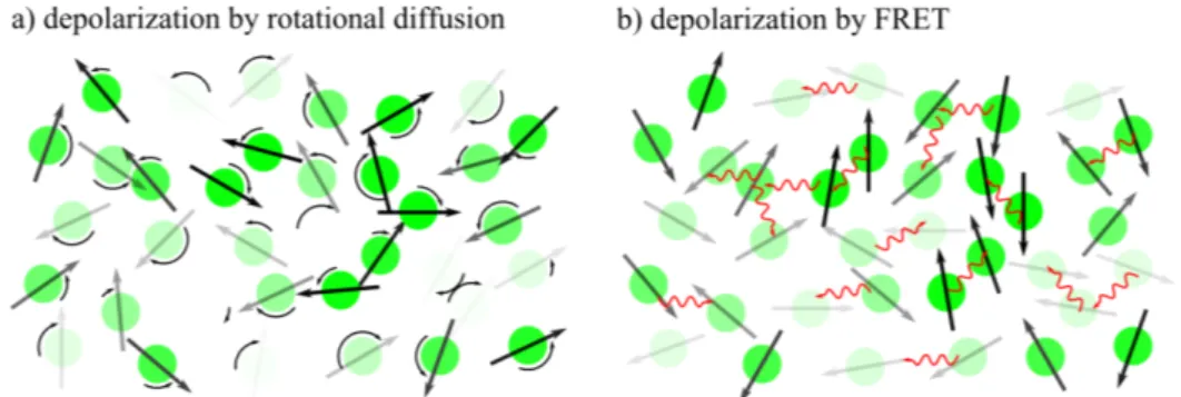
Fluorescence anisotropy is influenced by a number of processes that can lead to a depolarization of the light emitted by fluorophores. These processes can be intrinsic i.e. processes relying on the photophysical properties of the observed molecules or extrinsic, depending on the local environment (e.g. the rotational diffusion of the molecules or F¨ orster resonance energy transfer (see Figure 2.5)). In anisotropy imaging optical components of the microscope can also lead to a depolarization of the fluorescence signal.

Intrinsic sources of depolarization

Intrinsic sources of depolarization that depend on photophysical processes like photoselection can be best understood by considering the fluorescence of a single molecule. Assuming, the excitation light is polarized along the x

- axis and the dipole axis of the fluorescent molecule forms an angle Ψ with the x

-axis and an angle Φ with the x

-axis (see Figure 2.4), then the intensities I

and I

measured along the x

and x

-axis are given by:

I

= sin

Ψ sin

Φ, (2.3)

I

= cos

Ψ. (2.4)

However, in ensemble measurements multiple fluorophores contribute to

Figure 2.4: Schematic representation of an anisotropy measurement of a sin- gle molecule. The excitation polarization is parallel to the x

-axis. Intensities are measured along the x

- and x

-axis by placing a polarizer before the detec- tor oriented parallel and perpendicular with respect to the excitation beam.

Note that I

= I

.

the measured signal and the anisotropy will depend on the average orientation of the molecules. Therefore the average over the angles Ψ and Φ has to be calculated for randomly distributed fluorophores. This leads to:

r = 3 hcos

Ψi − 1

2 . (2.5)

Therefore the anisotropy is limited only by the value of hcos

Ψi originating from the photoselection [74]:

cos

Ψ

= R

0

cos

Ψf (Ψ) dΨ R

0

f (Ψ) dΨ , (2.6)

where f (Ψ) = cos

Ψ sin

ΨdΨ is the photon absorption probability for a random distribution of molecules. This leads to a fundamental emission anisotropy for an ensemble of randomly distributed molecules of r

= 0.4.

Extrinsic sources of depolarization

So far we have discussed intrinsic sources of depolarization. These sources

limit the fluorescence anisotropy fundamentally. Extrinsic factors can also

change the fluorescence signal, modifying the diffusion time, the fluorescence lifetime or the fluorescence polarization, thereby yielding information about the local environment of the fluorophore of interest.

One of the most important extrinsic sources of depolarization is the ro- tational diffusion of fluorophores. Molecules in a solution undergo Brownian motion, leading to translation and rotation of single fluorescent molecules. If

Figure 2.5: Schematic representation of depolarization by rotational diffusion and FRET. (a) Rotational diffusion leads to a depolarization of fluorescence light, if the fluorescent molecules are rotating within the time span of the fluorescence lifetime. (b) FRET between molecules leads to a depolarization of the emitted fluorescence.

a molecule rotates within the timespan of the fluorescence lifetime, the emis- sion dipole moment can rotate significantly between absorbing and emitting a photon. A molecule with a transition dipole moment initially aligned with the polarization of the excitation beam is then no longer aligned with the excitation light when emitting light. In a measurement of an ensemble of molecules, this leads to a depolarization of the emitted light. The rotational correlation time τ

of a molecule in a solution is defined as the time when the anisotropy has decayed to 1/e of its initial value [77]. The effect of rotational diffusion on the measured anisotropy is described by the Perrin equation [79]:

r

r = 1 + 6D

τ = 1 + τ

τ

, (2.7)

where r

is the fundamental emission anisotropy, D

the rotational diffusion

coefficient and τ the fluorescence lifetime. In cases where the fluorescence

lifetime is much shorter than the time scale on which rotational diffusion

takes place (τ << τ

) the fluorescence anisotropy is not altered by the rotational diffusion and the measured anisotropy is equal to the fundamental fluorescence anisotropy.

Another source of extrinsic depolarization of the fluorescence signal is F¨ orster resonance energy transfer. In F¨ orster resonance energy transfer en- ergy is transferred from an excited donor fluorophore to an acceptor chro- mophore. If the acceptor chromophore is also a fluorophore the measured fluorescence will be depolarized if the emission dipoles of the donor and ac- ceptor fluorophore are not parallel. Fluorescence energy transfer is discussed in more detail in section 2.1.3.

Optical sources of depolarization

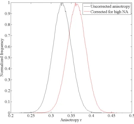
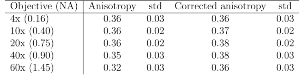
In an objective type TIRF-setup high NA objectives are used to tilt the excitation beam such that the excitation light can undergo total internal reflection (see section 2.2.3). However, high NA lenses alter the polarization and thereby lead to an artificial decrease of the fluorescence anisotropy by mixing of the polarization components [96]. The emission fluorescence as well as the excitation beam are subject to this mixing [10]. The purity of the polarization state of each partial ray decreases with its distance from the optical axis, making rim beams less suitable for polarization measurements.

However, these beams include information of molecule orientations along the optical axis and can be used to determine three-dimensional molecule orientations [61, 62]. High numerical aperture objectives lead to fluorescence anisotropy values that can be significantly lower than the actual value (see section 2.2.4).

2.1.3 F¨ orster resonance energy transfer

F¨ orster resonance energy transfer (FRET) is the non-radiative transfer of

energy from a donor fluorophore to an acceptor molecule, another chro-

mophore. Theodor F¨ orster first proposed a comprehensive theory describing

FRET [43, 44]. FRET is a dipole-dipole interaction, in which the donor and

acceptor molecule have to be in resonance with each other, meaning that

the emission and absorption spectra of the donor molecule and the accep- tor molecule have to overlap (Figure 2.6(a)). As a dipole-dipole interaction FRET varies inversely with the sixth power of the distance between donor and acceptor molecule. The rate k

of energy transfer is given by:

k

= 1 τ

R

r

. (2.8)

τ

is the fluorescence lifetime of the donor, R

is the F¨ orster radius at which the transfer efficiency drops to 50% and r is the distance between donor and acceptor molecule. The distance dependency is also evident in the energy transfer efficiency E:

E = k

(r)

k

(r) + k

(r) = R

R

+ r

, (2.9)

which is defined as the transferred energy divided by the total energy ab- sorbed by the donor. Figure 2.6(b) shows the transfer efficiency in de- pendence of the normalized distance. For commonly used fluorophores the F¨ orster radius lies within 5 nm to 10 nm, well below the resolution limit of a light microscope.

FRET can be best understood by considering a single donor-acceptor pair. The donor and acceptor molecule are separated by the distance r, the donor quantum yield is given by Q

and the extinction coefficient of the acceptor is (λ). Then the energy transfer rate can be written as [77]:

k

(r) = Q

κ

τ

r

9000 (ln10) 128π

N n

Z

F

(λ)

(λ) λ

dλ, (2.10) where n is index of refraction of the medium and N is Avogadro’s number.

F

(λ) is the fluorescence intensity of the donor in a range λ to ∆λ. The

area under F

(λ) is normalized to unity. κ describes the relative orientation

of the transition dipoles of the donor and acceptor molecule. The integral

in equation (2.10) is called the overlap integral J (λ). The overlap integral

depends only on the total intensity of the transition dipole moments and

does not include the orientation factor κ

, which is present in the transfer

(a) (b)

Figure 2.6: (a) Principle of F¨ orster resonance energy transfer. The donor fluorophore in the excited state may relax to its ground state by emission of a photon. If an acceptor molecule is in close proximity the energy of the donor can be transferred to the acceptor molecule by a dipole-dipole interaction.

For this to happen the donor and acceptor molecule have to be in resonance meaning the emission spectrum of the donor must overlap with the excitation spectrum of the acceptor molecule. (b) Energy transfer efficiency E as a function of

0

. At the F¨ orster radius R

the efficiency drops to 50%

rate. κ

is given by:

κ

= (sin Θ

sin Θ

cos Φ − 2 cos Θ

cos Θ

)

. (2.11) The angle Θ

is the angle of the emission transition dipole of the donor mo- lecule and Θ

is the angle of the absorption transition dipole of the acceptor molecule with the vector joining these two molecules. Φ is the angle between the planes in which the transition dipole moments of donor and acceptor lie (see Figure 2.7).

For a random distribution of transition dipoles the orientation factor is κ

=

, where it is assumed that the distance between the two dipoles is large compared to the charge separation. For perpendicular transition dipole moments κ

vanishes and no energy is transferred; for parallel dipoles κ

= 4.

FRET can be detected by several imaging techniques as it directly influ-

ences the photophysics of fluorophores. The energy transfer from the excited

Figure 2.7: Schematic representation of the relative orientation of the donor and acceptor molecule. Donor and acceptor are separated by the distance r. The orientation factor κ

depends on the relative orientation of donor and acceptor molecule. κ

is maximal if the emission transition dipole of the donor molecule is parallel to the absorption dipole of the acceptor molecule and vanishes if they are oriented perpendicular.

state of the donor molecule to the excited state of the acceptor molecule leads to a decrease in the number of photons emitted by the donor. At the same time the acceptor molecule is excited and, in case the acceptor is another fluorophore, will fluoresce. FRET can therefore be detected by monitoring changes in the intensities of the donor and/or the acceptor by various meth- ods [48].

As FRET influences the excited state lifetime, fluorescence lifetime mea-

surements can also be used to detect FRET. Lifetime measurements are

independent of the fluorophore concentration and are therefore often pre-

ferred over intensity based measurements. For an extended review of imaging

techniques the reader is referred to [70]. In this thesis only anisotropy mea-

surements will be reviewed in detail. FRET leads to a depolarization of the

overall fluorescence, due to the relative orientation of the donor and acceptor

molecule. The dipole-dipole interaction shows a cosine squared dependency

on the angle between acceptor and donor of the FRET-pair, thereby allowing a range of relative orientations for which FRET can occur. An acceptor mo- lecule with an emission dipole moment which is not parallel to the emission dipole moment of the donor will lead to a depolarization of the fluorescence signal (Figure 2.5). Compared to other techniques, anisotropy measure- ments allow the detection of homo-FRET, the transfer of energy between identical fluorophores, providing a straightforward approach for measuring homo-dimerization and oligomerization of proteins [120, 18, 19, 17].

2.2 Microscopy

A microscope enables the user to observe objects and processes on sub- micrometer length scales. The first microscopes were built in the late 16

and early 17

century, and have been widely used in the biological sciences since then. Fluorescence microscopy is of major interest as it allows specific tagging of the molecules of interest. However, the limiting factor in micros- copy is the optical resolution which restricts the size of resolvable objects to roughly 600 nm along the optical axis and 200 nm laterally [57].

2.2.1 Resolution limit

An object which is much smaller than the wavelength of light disturbs the wavefront of light incident on this particle. This object is, according to the Huygens-Fresnel principle, the source of a spherical wave. The intensity of this scattered wave is dependent on the size of the object. However, as long as the object is much smaller than the wavelength of light, the scattered wave will always be a spherical wave independent of the shape of the object. No information about the shape of the object is thus transported by the wave of light. Ernst Abbe first described when the shape of a microscopic object is resolvable [1] and thereby determined the resolving power of optical micro- scopes. In his work Abbe considered a grating imaged by a lens (Figure 2.8).

The grating, illuminated by a light source, forms a diffraction pattern with

a central intensity maximum of zeroth order, and higher order maxima next

to it. The angle of diffraction of these higher order maxima depends on the separation of the grating elements and becomes greater with smaller separa- tion of the elements. To gain information about the distance of the grating

Figure 2.8: Abbe diffraction limit. A grating is imaged on screen by a microscope objective. Light incident on a grating will be diffracted and form a central maximum. A first order maximum will occur at an angle Θ, which depends on the distance of the grating elements d. To resolve the grating the microscope objective has to capture at least the first order maximum of the diffracted beam. The resolution of an optical microscope therefore depends on the range of angles which are accepted by the objective.

elements the lens must capture at least the first order maximum. Abbe found that the minimal distance d

between the grating elements, such that they could be distinguished from one another, is

d

= λ

2n sin Θ , (2.12)

the resolution limit according to Abbe. Herein, n is the index of refraction of

the surrounding medium and Θ is the half-angle of the cone of light which can

enter the lens. NA = n sin Θ is called numerical aperture and is a measure

for the range of angles of light that can be captured by a lens.

Shortly after Abbe, Lord Rayleigh described the interference patterns of two point sources of light separated by a distance d and imaged by a lens [84]. The light emitted by each point source will be diffracted by the aperture of the lens according to the Huygens-Fresnel principle, forming a diffraction pattern on a screen. The image of a single point source is forming a maximum of zeroth order at the center and concentric rings of higher orders around this central maximum: the Airy diffraction pattern. According to the Rayleigh- Criterion the two points can be distinguished if the zeroth order maximum of one light source just overlaps with the first minimum of the second point source. For any distance smaller than this the two point sources are not

Figure 2.9: Rayleigh criterion. a) The diffraction patterns of two resolved point sources of light. b) If the maximum of zeroth order just overlaps with first minimum of the second diffraction pattern, the image is just resolved. c) If the diffraction patterns overlap completely, the image is not resolved.

resolved (Figure 2.9). The resolution limit given by the Rayleigh-limit is [26]:

d = 0.61 · λ

n sin Θ . (2.13)

It is worth noting, that λ is the emitted light wavelength and, unlike in Abbes

description, not the illumination wavelength. The intensity distribution of a

point source formed by a microscope in the image plane is called the point

spread function (PSF). The image formation in a microscope can then be

understood as a convolution of the PSF of the microscope with the object

shape [71].

2.2.2 Localization based super-resolution techniques

The diffraction of light fundamentally limits the resolution in optical micros- copy. In recent years several methods have been described to circumvent the lateral diffraction limit in microscopy. These techniques rely on the spatial patterning of the illumination light [50], the spatial patterning of the exci- tation light and the nonlinear response of fluorescent molecules [51, 114] or the temporal patterning of the emission of fluorophores upon a nonlinear switching behavior [23, 98, 60, 55, 35, 82]. The latter include also techniques known as localization microscopy.

Localization based microscopy techniques are capable of achieving optical resolution beyond the diffraction limit of light. These techniques rely on the sequential imaging of single molecules. Fluorescent molecules are switched between a non-fluorescent state and a fluorescent state. Instead of imaging all fluorescent molecules at once, a time series is recorded. In each image of the time series only a small subset of molecules is switched to the fluorescent state. Optimally each molecule is imaged once with no other molecule fluo- rescing at the same time in the same diffraction limited region. Thus, these techniques can be regarded as a time division multiplexed recording of an im- age: Multiple fluorescent molecules residing in the same diffraction limited spot emit fluorescence light at different time points and thus can be distin- guished. However, compared to common time division multiplexing systems in telecommunication, multiplexing in localization microscopy is a stochastic process as the stochasticity of switching molecules from an non-fluorescent

“off-state” to a fluorescent “on-state” is used to keep the density of fluores- cent molecules low. Therefore localization based super-resolution microscopy techniques strongly depend on the photophysical and photochemical prop- erties of fluorescent molecules and are often hampered by their non-ideal switching and blinking behavior [112, 7, 8, 27].

The image of a single molecule is the convolution of the object shape with

the point spread function of the microscope. A single molecule imaged by an

optical microscope can be regarded in good approximation as a point source

of light as it is much smaller than the wavelength of the emitted fluorescence

light. The light emitted by this molecule will be diffracted by the microscope and form an Airy-diffraction pattern [26]. The diffraction pattern can be approximated by a two dimensional Gaussian distribution [121] with a width given by the point spread function of the microscope. The position of the centroid of the fluorescent molecule can be determined by fitting a Gaus- sian function to this intensity distribution. For a two dimensional Gaussian function centered at x

, y

on a CCD camera the intensity I

is given by:

I (r) = I

e

(x−x0)2

2s2 +^(y−y0)2

2s2

, (2.14)

where I

is the amplitude and s is the standard deviation resulting from the point spread function. The standard error of determining the centroid is given by [109]:

(∆x)

= s

+ a

/12

N + 8πs

b

a

N

, (2.15)

where a is the size of a pixel measured in the sample plane, b is the background noise and N is the number of photons collected. The standard error is mainly limited by the number of photons collected. For a high enough number of photons

(∆x)

can be approximated by

(∆x)

≈

N

. For N = 500, a wavelength of λ = 590 and an objective with N A = 1.45 this results in a standard error of

(∆x)

≈ 4nm, which is much smaller than the diffraction limit of light. Thus, the position of a single fluorescent molecule can be determined with a precision exceeding the optical resolution limit in microscopy by far.

Assuming two molecules which are separated by a distance smaller than

the diffraction limit (Figure 2.10), one can see the benefits of sequentially

localizing single point emitters. If the two molecules emit fluorescence light

at the same time, the image will be the result of the convolution of the two

points with the PSF of the microscope and it is not possible to resolve the two

molecules. In a sequential imaging scheme only one molecule will fluoresce at

a given time point and its position can be determined. The second molecule

will be imaged at a later time point. As long as the distance between the

two molecules is larger than the localization precision, the two molecules can

Figure 2.10: Localization of a single molecule by sequential imaging. Two fluorescent molecules and their intensity profiles. The two molecules are unre- solved if the distance between their centers is less than the diffraction limit. If one of the molecules is imaged at a time point t

its position can be determined by localizing the center of its intensity profile. At a later time point t

only the second molecule emits fluorescence and can be localized. The localization precision exceeds the diffraction limit, thus a sum image of the positions will yield a super-resolution image.

be distinguished by their positions.

In a typical fluorescence microscopy measurement all fluorophores are in a fluorescent state. However, for localization microscopy based super- resolution techniques most of the fluorophores must be in a non-fluorescent dark state, such that the mean distance between two fluorescent molecules is greater than the diffraction limit of light [40]. If this holds true, the probabil- ity of finding two or more fluorescent molecules residing in the same diffrac- tion limited region is small and single molecules can be imaged and localized.

The imaging of a sparse subset of fluorescent molecules can be achieved by

using photoactivatable fluorophores. These fluorophores are stochastically

activated from an initially non-fluorescent state usually by illumination with

light of a specific wavelength. Molecules in an active state show fluorescence

upon excitation with light of a different spectral region. Sparse activation

of the fluorophores allows for imaging of single fluorescent molecules. These

molecules are then photobleached or deactivated by the readout light (Figure

2.11). To image a sufficient amount of molecules within the sample the mol-

Figure 2.11: Principle of photo-activated localization microscopy. (a) Pho- toactivatable fluorescent molecules are in an non-fluorescent “off state”. (b) Irradiation with light of a specific spectral range (in most cases UV-light) ac- tivates molecules. (c) Molecules now in an “on-state” will show fluorescence upon excitation. By activating only a small subset of molecules, the mean distance of fluorescent molecules will be much larger than the diffraction limit of light. (d) Molecules are imaged until they are bleached. A new subset of molecules is activated. (f) The cycle of activation and imaging is repeated until a sufficient number of molecules is localized.

ecules are usually continuously activated and read out at the same time. In a

post-processing step the positions of the recorded single molecules are local-

ized and an image of the molecule positions is reconstructed. The resolution

of the reconstructed image is given by the localization accuracy of the sin-

gle molecule positions as well as the density of the fluorophores. According

to the Nyquist-Shannon sampling theorem [102] the distance between two

neighboring molecules has to be at most half the distance of the desired reso-

lution, otherwise structures on the length scale of the desired resolution will

not be resolved [92]. For instance, to achieve 20 nm resolution, the structure

has to be sampled at 10 nm in every direction.

2.2.3 Total internal reflection

So far we described methods to reduce the lateral resolution limit in opti- cal microscopy. Localization based techniques can be extended to improve the resolution along the optical axis of the microscope [66, 65, 72, 103, 93].

However, these techniques require the use of additional optics in the emis- sion pathway. In conventional wide-field setups the sample is excited outside the focal plane, thereby introducing background fluorescence to the mea- surement. The region which is excited can be reduced by using total internal reflection fluorescence microscopy [5]. In total internal reflection fluorescence microscopy the evanescent field of an electro-magnetic field is used to excite fluorescence. The word evanescent derives from the latin word “evanescere”

which means vanishing. Therefore, in total internal reflection fluorescence microscopy (TIRF microscopy) “vanishing” waves of light are used to excite fluorescent molecules. Evanescent waves can be described by plane waves of the form:

E ~ = e

(

) . (2.16) The main characteristic of an evanescent wave is the presence of at least one imaginary component of the wavevector ~k. The wave along the direc- tion of this imaginary component decays exponentially rather than propa- gating along this direction. Furthermore evanescent waves never occur in homogeneous media, their generation requires the interaction of light with inhomogeneities.

An evanescent wave is the result of light undergoing total internal reflec- tion (Figure 2.12). Light being incident on an interface of two media with refractive indices n

and n

is partially reflected and refracted. Snell’s law states:

n

sin (Θ

) = n

sin (Θ

) , (2.17)

where Θ

and Θ

are the angle of incidence and refraction, each measured

from the normal of the interface. Light can be totally reflected if it propagates

from an optically denser medium to an optically less dense medium, so that

n

is greater than n

. Light propagates tangential to the interface at an

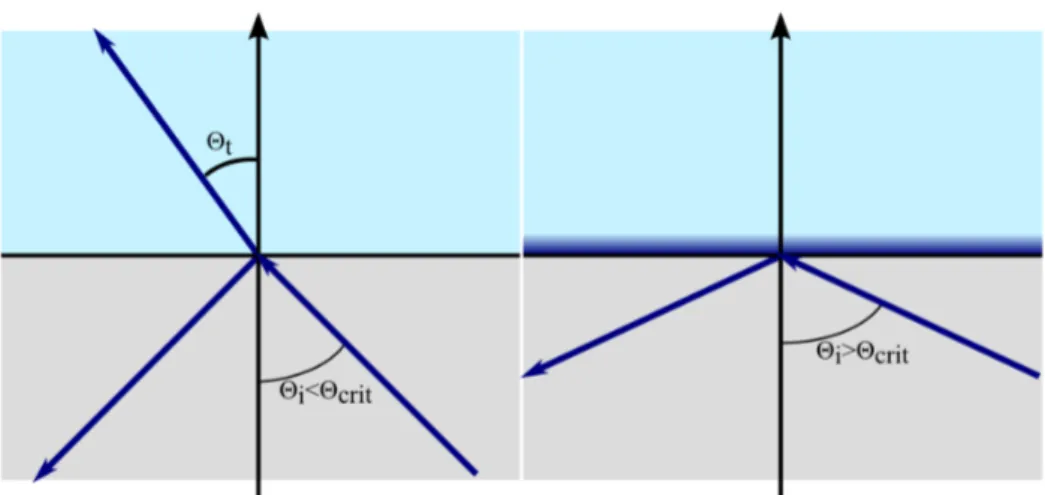
Figure 2.12: Light coming from a medium with an index of refraction n

and entering a medium with a refractive index n

with n

> n

undergoes total internal reflection if the incidence angle Θ is greater than the critical angle Θ

. At Θ

the angle of refraction is 90

, thus light is travelling parallel to the interface between the two media. For light undergoing total internal reflection an evanescent field is generated in the second medium. The evanescent wave vanishes exponentially with the distance from the interface where light is totally reflected.

incidence angle called the critical angle Θ

when Θ

becomes 90

. The critical angle then can be derived from equation 2.17 and is given by:

Θ

= arcsin n

n

. (2.18)

For any incidence angle Θ

exceeding the critical angle no light will enter the optically less dense medium and but will be totally reflected. The net energy flow through the interface will vanish, however the electromagnetic field in the second medium will not disappear but decay exponentially in the direction normal to the interface. For light undergoing total internal reflection at an interface in the xy-plane and the plane of incidence in the xz-plane, the evanescent wave intensity is given by:

I (z) = I (0) e

, (2.19)

where the penetration depth d is given by:

d = λ

4π

1

p n

sin

Θ − n

. (2.20) λ

is the wavelength of the incidence light [14].

In microscopy the evanescent wave is used to excite small regions just above the coverglass/sample interface. The penetration depth is greatly re- duced due to the exponential decay of the evanescent wave. For green fluores- cent protein excited at 476 nm and with a high NA-objective of 1.45 an inci- dent angle of 72

is achievable. With an index of refraction of n

= 1.52 and n

= 1.33 the penetration depth is d = 67 nm. The plasma mem- brane of a cell has a thickness of roughly 5 nm [3] and is close to the cover- glass (approximately 30 nm [73]). Fluorescently tagged proteins residing in the plasma membrane can thus be excited efficiently by an evanescent wave, whereas fluorescent background from cytosolic proteins is greatly reduced.

Experimentally TIR-illumination in fluorescence microscopy can be real-

ized in several ways, the two most common schemes are through objective

type illumination and prism-based illumination. In a prism-based setup a

prism is used to couple light to the interface where total internal reflection

takes place (Figure 2.13), fluorescence is then collected by microscope ob-

jective usually opposite to the prism. Prism type TIRF-setups offer better

control over the incidence angle and thus over the penetration depth of the

evanescent wave than objective type setups [101]. However, the sample acces-

sibility is greatly reduced: The sample has to be kept between two coverslides

allowing for excitation only in close proximity of the upper slide which is con-

nected to the prism. The distance between the two cover glasses has to be

reduced if an objective with a high numerical aperture and low working dis-

tance is used. Objective type TIRF setups use a high-NA objective which

allows for angles of excitation above the critical angle. Light is focused to

the back focal plane of the microscope objective. A translation of the beam

in the back focal plane away from the lens center leads to tilting of the ex-

citation beam, which can be used to achieve total internal reflection. For

total internal reflection to occur on a glass/water interface with refractive

Figure 2.13: Experimental realization of TIR illumination in fluorescence microscopy. In a prism type TIRF setup (left) the light is coupled to the sample by a prism. The excitation beam undergoes total internal reflection at the coverglass. Light is collected by an objective which is positioned opposite to the prism. In an objective type TIRF setup (right), the excitation beam is focused off center to the back focal plane of a microscope objective. The objective tilts the excitation beam so it is incident on the cover glass with an angle exceeding the critical angle. Fluorescence light is collected by the same objective.

indices of n

= 1.52 and n

= 1.33 the critical angle is Θ

= 61.0

. For an immersion medium with a index of refraction of n

= 1.518 this results in a minimal numerical aperture of N A = 1.33. TIRF-objectives must therefore have a numerical aperture which exceeds 1.33. Commercially available objectives have a numerical aperture ranging from 1.40 to 1.65.

Objective based TIRF setups use the same objective for exciting the sample and collecting the fluorescence emission, thus no special considerations about the sample design and accessibility have to be taken into account.

2.2.4 Fluorescence anisotropy microscopy

So far we described methods to measure light intensity with high spatial

resolution. As described in section 2.1.2 fluorescence anisotropy is a measure

of the polarization of light emitted by an ensemble of fluorescent molecules,

which can also be observed with a microscope. For the measurement of

fluorescence anisotropy the sample is excited by polarized light and the light

intensities polarized parallel and perpendicular to the excitation light are measured. Fluorescence anisotropy is defined as:

r = I

− I

I

, (2.21)

where I

is the intensity measured parallel to the excitation light and I

the light intensity perpendicular to the excitation light. The total intensity I

is given by:

I

= I

+ 2I

. (2.22)

The normalization of equation (2.21) by the total intensity leads to a dimen- sionless value for the anisotropy r, which is independent of the fluorophore concentration. The factor 2 in the total intensity results from the three in- tensity components I

, I

and I

along the axes x, y and z (see Figure 2.2) contributing equally to the total intensity. For a rotation symmetric emission of fluorescence around the z-axis I

equals I

with I

= I

this leads to

I

= I

+ I

+ I

= I

+ 2I

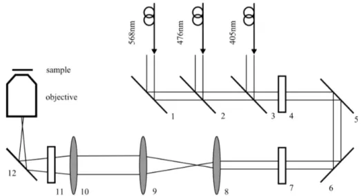
. (2.23) Figure (2.14) shows a schematic diagram of an anisotropy setup with a con- ventional wide field microscope. The sample is excited by a light source with a fixed linear polarization. The intensities polarized parallel and perpen- dicular to the excitation light are split by a polarizing beam splitter. Each channel can then be imaged separately by a camera.

High numerical aperture objectives

In fluorescence anisotropy microscopy special care has to be taken when using high numerical aperture microscope objectives. High NA-objectives can alter the polarization of the excitation as well as the polarization of the emission light due to their large angle of acceptance [20, 69] and lead to measured fluorescence anisotropies which are significantly lower than the actual fluorescence anisotropy.

The description in this thesis is based on [9, 10], which does not incorpo-

Figure 2.14: Schematic representation of a fluorescence anisotropy measure- ment with a wide field microscope. The sample is illuminated with linearly polarized excitation light (polarization points into the drawing plane). Fluo- rescence from the sample is separated from the excitation light by a dichroic mirror. The emitted light is then split by a polarizing beam splitter into light with polarization parallel (I

)and perpendicular (I

) to the excitation light.

An image of each channel is recorded.

rate any polarization effect on the excitation part as for widefield illumination the tipping and tilting of the polarization is negligible. In TIRF microscopy the s-polarized incident light will not be influenced by any high-NA-effect (see section 2.2.3) and thus the correction described in [9, 10] is also appropriate.

The influence of an objective with a high numerical aperture results from tipping and tilting of light by the objective. The total fluorescence collected by the objective is given by [9, 10]:

F

= k

F

+ k

F

+ k

F

, (2.24)

F

= k

F

+ k

F

+ k

F

, (2.25)

where k

, k

, k

are weighting factors accounting for the numerical aperture

of the microscope objective. With Θ being the half angle of the cone of light

Figure 2.15: Detection of fluorescent molecules by a high-NA lens. The polarization is tilted by the lens such that light polarized along the z-axis will be detected. Molecules of all orientations will contribute to the fluorescence signal. This polarization mixing leads to a reduced anisotropy value.

accepted by the microscope objective k

, k

, k

can be rewritten as:

k

= 1

6 · 2 − 3 cos Θ + cos

Θ

1 − cos Θ , (2.26)

k

= 1

24 · 1 − 3 cos Θ + 3 cos

Θ − cos

Θ

1 − cos Θ , (2.27)

k

= 1

8 · 5 − 3 cos Θ − cos

Θ − cos

Θ

1 − cos Θ . (2.28)

The fluorescence anisotropy then can be calculated for a distribution of

randomly oriented molecules by using the corrected intensities:

F

= k

F

− k

F

k

k

+ k

− k

k

− k

, (2.29) F

= (k

+ k

) F

− (k

+ k

) F

k

k

+ k

− k

k

− k

. (2.30)

2.2.5 TIRF anisotropy

The use of an evanescent wave in fluorescence anisotropy measurements re- duces the signal from out-of-focus light greatly due to the reduced penetra- tion depth of the evanescent field. In section 2.2.3, the generation of an evanescent wave has been described. To make use of an evanescent wave in fluorescence anisotropy microscopy the polarization of the evanescent field has to be taken into account. The electric field components of an evanescent wave at the interface were total internal reflection takes place (z = 0) are given by [13, 12]:

E

= (2 cos Θ) sin

Θ − n

n

cos

Θ + sin

Θ − n

A

e

(

) , (2.31a) E

= 2 cos Θ

(1 − n

)

A

e

, (2.31b)

E

= 2 cos Θ sin Θ

n

cos

Θ + sin

Θ − n

A

e

, (2.31c)

with

δ

≡ tan





sin

Θ − n

n

cos Θ



 , (2.32a)

δ

≡ tan





sin

Θ − n

cos Θ



 . (2.32b)

An incident beam with a polarization direction parallel to the plane of

incidence (p-polarization) and no polarization component perpendicular to the plane of incidence (A

= 0) results in an evanescent wave with elec- tric field components in x and z direction, with x being longitudinal. The phase shift of

between the x- (equation (2.31a)) and z-component (equation (2.31c)) results in a whirling of the electric field around the z-axis (Figure 2.16). For an incidence beam with a polarization purely perpendicular to

Figure 2.16: Polarization of the evanescent wave. A light beam undergoes total internal reflection. For a s-polarized incident light beam, the evanescent wave polarization is not altered and is polarized in the sample plane. A p- polarized incident beam results in an evanescent field with components in z- and x-directions. The phase difference of the x- and z-component (see Equa- tion (2.31)) causes the evanescent field to whirl around the z-axis (adapted from [11]).

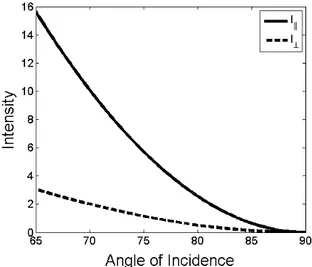
the incident plane (s-polarization) results in an evanescent electric field with a y-component and thus is polarized in this direction. It is important to note that the penetration depth d is independent of the polarization of the incident light, however, I (0) does show a dependency on the polarization as well as on the angle of the incidence light [13, 11] (see Figure 2.17):

I

(0) = A

2

(4 cos

Θ) 2 sin

Θ − n

n

cos

Θ + sin

Θ − n

, (2.33a) I

(0) = |A

|

4 cos

Θ

1 − n

, (2.33b)

where A

2

and |A

|

are the incident intensities and n =

2

.

Figure 2.17: Intensities I

(0) and I

(0) plotted for different incidence angles Θ

beyond the critical angle Θ

= 61.5

with n

= 1.33 and n

= 1.52.

A

2

and |A

|

are set to 1.

Due to its unique polarization states TIRF is well suited for anisotropy measurements. It allows for a purely transversal polarization in the sample plane as well as for a polarization state mainly along the optical axis of the microscope. Thus, probing any polarization state is possible without loosing the wide field capabilities. TIRF polarization measurements have been carried out as intensity measurements in dependence of the orientation of the polarization of the excitation light [9, 15].

2.3 Review of fluorescence anisotropy imag- ing literature

Despite the possibility of resolving clustering and dimerization by measuring

homo-FRET [29], fluorescence anisotropy in combination with imaging has

not been widely exploited yet. In particular fluorescence anisotropy measure-

ments with TIRF microscopy have been seldomly used. Only recently fluo-

rescence anisotropy in TIRF was used to investigate the homodimerization of

Amyloid Precursor Protein [36]. Prior polarization measurements in TIRF

were mostly carried out as intensity measurements, probing the molecules of interest with the different polarization states of the exciting evanescent field [9, 15]. Further polarization measurements in TIRF were carried out to determine the organization of F-Actin [42] and the tilting and wobbling of Myosin V [22], however these measurements used a complex prism-type setup.

On a single molecule level orientation measurements are well known. Ha et al. presented orientation measurements by probing the absorption dipole moment of a single TexasRed molecule [52], polarization measurements were used to measure 2d molecule orientations [54] and in combination with spatial sampling of the Fourier components to measure 3d orientations [62, 45]. The defocused image of single molecules can also be used to determine 3d molecule orientations [25].

However, TIRF excitation was rarely used in single molecule orientation measurements. Orientation measurements in super resolution microscopy were mostly carried out by conventional wide field excitation measuring the polarization of the excitation light [46, 108].

Recently the polarization modulation in TIRF by rotating the excitation

beam in the backfocal plane of the microscope objective was used to measure

molecule orientations by probing the absorption dipole of single organic dye

molecules [80].

Experimental realization of TIRF-anisotropy

This chapter describes the requirements for a TIRF anisotropy microscope,

which is used for ensemble measurements as well as for single molecule mea-

surements. The basic components of the microscope are discussed in de-

tail. The central part, the microscope frame itself, is a commercially avail-

able inverted microscope. To implement polarized TIRF, the excitation and

emission paths of the microscope are modified. In the next sections these

modifications are discussed separately.