Postglacial paleoenvironmental history of the Southern Patagonian Fjords at 53°S
I n a u g u r a l - D i s s e r t a t i o n zur
Erlangung des Doktorgrades
der Mathematisch-Naturwissenschaftlichen Fakultät der Universität zu Köln
vorgelegt von Jean P. Francois S.
aus Santiago de Chile
Köln, 2014
Berichterstatter: Prof. Dr. Frank Schäbitz
Prof. Dr. Olaf Bubenzer
Vorsitzender der
Prüfungskommission: Prof. Dr. Martin Melles
Tag der mündlichen Prüfung: 7. Juli. 2014
A mi familia
i Abstract
Southern Patagonia (50°-56°S) is as key region for paleoenvironmental studies, in particular, for addressing fundamental paleoclimatic and paleoecological questions. This is due to a number of physical and biotic characteristics of the region: (i) its location allows to examine and reconstruct changes of the Southern Westerly Wind (SWW) belt, (ii) the presence of the Andes, which intercepts the flux of the SWWs creating a strong orographic precipitation gradient on a west-east axis, and (iii) consequently the development and succession of distinct ecosystems along this gradient.
This thesis aims to investigate the vegetational history of Southern Patagonia through space and time and assess the various physical parameters that shaped these environments. Therefore, a comprehensive study of the modern vegetation and pollen rain in the Fjords at 53°S was undertaken. Additionally, a new paleoenvironmental record was acquired from the Tamar Lake (52°54’S; 73°48’W) and was analyzed using geochemistry and pollen analysis. Lastly, the Tamar and other regional paleorecords located along a west-east transect at 53°S were compared using multivariate analyses (PCA, DCCA, rarefaction) in order to develop a comprehensible postglacial history of S. Patagonian ecosystems.
The main vegetation types (i.e. Magellanic Moorland, Evergreen forest, Deciduous forest and Patagonian Steppe) occurring along this west-east transect are clearly identified in the modern pollen rain. Redundancy analysis suggests that modern pollen spectra from the different ecosystems are closely linked with the precipitation and temperature gradient occurring at 53°S. The pollen record from Tamar covering the last 16,000, indicates the development of a heath and grassland between 16 – 13.6 kyr BP, followed by the spread of scrublands and Nothofagus woodlands after 13.6 kyr BP, suggesting a shift from cold/dry to a more warm/wet climate. The Holocene is characterized by a succession of distinctive forest types, which begins with the development of Nothofagus forests (~11.8 – 8.5 kyr BP), followed by Nothofagus-Drimys forests (~10.3 – 6.2 kyr BP), and culminating in mixed temperate evergreen forests (~6.2 kyr BP to present). These changes in vegetation suggest a shift in the intensity of the SWWs and in temperature during the postglacial, accounting for a windy/warm early Holocene. Mass wasting events, well-developed soils and dense vegetation are characteristic for this period. Finally, the findings from the paleoecological reconstruction along Southern Patagonia, reveal substantial differences in the vegetation history (i.e. compositional changes, turnover and palynological richness) of the ecosystems located west and east of the Andes during the postglacial. The response of the ecosystems to environmental forcing (climatic and non- climatic) differs significantly along this transect.
This study reveals the complex interplay between abiotic and biotic factors (e.g. temperature,
precipitation, soil development, species competition) in the evolution of the ecosystems of Southern
Patagonia over time. The ecosystems respond sensitively to environmental (climatic and non-
climatic) forcing, but differ significantly in their resilience depending on intrinsic characteristics. In
light of increasing anthropogenic impact and ongoing climate change, these findings offer important
insights in the evolution of regional ecosystems that could be used in planning conservation projects.
ii Kurzzusammenfassung
Süd-Patagonien (50°-56°S) ist eine Schlüsselregion für Paläoumwelt-Studien, insbesondere im Fokus grundlegender paläoklimatischer und paläoökologischer Fragestellungen. Dies liegt an einer Reihe von typischen physisch-geographischen und biotischen Merkmalen der Region: (i) ihre Lage gestattet die Überprüfung und Rekonstruktion der Änderungen der latitudinalen Position der südlichen Westwindzone (SWW), (ii) der Andenkordilliere, die für die SSW eine Barriere darstellt und für einen starken orographischen Niederschlagsgradienten entlang einer West-Ost-Achse sorgt, und folglich, (iii) der Entwicklung und Sukzession unterschiedlicher Ökosysteme entlang dieses Gradienten.
Ziel dieser Arbeit ist die raum-zeitliche Untersuchung der Vegetationsgeschichte von Süd- Patagonien und die Bewertung von verschiedenen natürlichen Parametern, die diese Umwelt prägt.
Dazu wurde eine umfassende Studie über die rezente Vegetation und den rezenten Pollenniederschlag in den Fjorden auf 53°S vorgenommen. Zusätzlich wurde ein neuer Paläoumwelt-Datensatz aus Seesedimenten des Tamar-Sees ( 52°54‘S , 73°48’W ) mittels Geochemie und Pollenanalyse ausgewertet. Anschließend wurden die Tamar-Daten mit anderen regionalen Paläo-Datensätzen entlang eines West-Ost-Transekts auf 53°S unter Anwendung multivariater Analysen (PCA, DCCA, rarefaction) verglichen, um einen Überblick zur nacheiszeitlichen Entwicklungsgeschichte süd-patagonischer Ökosysteme zu erstellen.
Die Hauptvegetationstypen (u.a. Magellanisches Moorland, immergrüne Wälder, laubwerfende Wälder und patagonische Steppe), die entlang dieses West-Ost-Transekts auftreten, prägen sich deutlich im rezenten Pollenniederschlag aus. Redundanz-Analysen deuten darauf hin, dass rezente Pollenspektren aus den verschiedenen Ökosystemen eng mit dem Niederschlags- und Temperaturgefälle auf 53°S zusammenhängen. Der Pollennachweis des Tamar-Sees für die letzten 16,000 Jahre zeigt die Entwicklung von Heide- und Grasland zwischen 16 bis 13.6 kyr BP, gefolgt von der Ausbreitung von Buschland und Nothofagus –Wäldern nach 13.6 kyr BP, was auf eine Verschiebung von kalt / trockenem zu einem wärmeren / feuchten Klima schließen lässt.
Das Holozän ist durch die Entwicklung einer Reihe von markanten Waldtypen gekennzeichnet.
Anfänglich durch die Ausdehnung von Nothofagus-Wälder charakterisiert
(~11.8 – 8.5 kyr BP), folgt auf diese Phase die Ausbreitung von Nothofagus-Drimys- Wäldern (~10.3 bis 6.2 kyr BP), welche schließlich zu den heutigen gemäßigten, immergrünen Mischwäldern führt (~6.2 kyr BP bis heute). Diese Veränderungen in der Vegetation deuten auf eine Verschiebung der Intensität der SWW und der Temperatur im Postglazial hin, gefolgt von einem windigen / warmen Frühholozän. Hangrutschungen, gut entwickelte Böden und dichte Vegetationsbedeckung sind charakteristisch für diesen Zeitraum. Zusammenfassend ergeben die Erkenntnisse aus der Paläoumwelt-Rekonstruktion in Süd-Patagonien, dass sich die nacheiszeitliche Vegetationsgeschichte (d.h. Änderungen der Vegetationszusammensetzung, Artenwechsel und Pollen-Diversität) der Ökosysteme westlich und östlich der Anden erheblich voneinander unterscheiden. Die Reaktion der Ökosysteme auf Umweltveränderungen (klimatischer und nicht- klimatischer Natur) unterscheidet sich signifikant entlang des Transekts.
Diese Studie verdeutlicht das komplexe Zusammenspiel zwischen abiotischen und biotischen Faktoren (z.B. Temperatur, Niederschlag, Bodenentwicklung, Konkurrenz) in der Evolution der Ökosysteme von Süd-Patagonien über einen langen Zeitraum hinweg. Die Ökosysteme reagieren empfindlich auf Umweltveränderungen (klimatischer und nicht-klimatischer Natur). Abhängig von ihren intrinsischen Merkmalen, unterscheiden sich aber deutlich in ihrer Anpassungsfähigkeit.
Angesichts des zunehmenden anthropogenen Eingriffs und dem fortschreitenden Klimawandel,
liefern diese Erkenntnisse wichtige Einblicke in die Entwicklung der regionalen Ökosysteme, was
für die Planung von Naturschutzprojekten Beachtung finden sollte.
iii Acknowledgments
First of all, I would like to thank my supervisor, Prof. Dr. Frank Schäbitz (University of Cologne) who provided me the support during all these years of thesis work. Likewise, my gratitude is extended to Prof. Dr. Rolf Kilian (University of Trier) for sharing data from Tamar Lake but more important for his advice and big influence in my work, without which it would not have been possible to make this thesis. I thank the Deutscher Akademischer Austausch Dienst (DAAD) and the Comisión Nacional de Investigación Científica y Tecnológica (CONICYT) for funding this my thesis (DAAD-CONICYT Stipendium, 07-DOCDAAD-08), and Prof. Dr. Olaf Bubenzer for agreeing to review this thesis.
I also whist thanks to the Drs. Frank Lamy (AWI Bremerhaven), Helge Arz, Jerome Kaiser (Leibniz Institute for Baltic Sea Research, Warnemünder) and Flavia Quintana (University of Bariloche) for their helpful ideas to my work. In addition, I would like to thank all colleagues and friends from the Laboratory of Palynology and the department of Geographie und Ihre Didaktik of the Universität zu Köln: Karsten Schittek, Jonathan Hense, Verena Foerster, Jan Wowrek, Tsige Gebru-Kassa, Maria Papadopoulou, Mark Bormann, Jonas Urban, Wilfried Schulz, Michael Wille, Steffi Reusch, René Kabacinski, Carina Casimir, Markus Dzakovic and Dominik Berg for stimulating conversations, bright ideas, its invaluable help in the laboratory and for numerous extra curriculum activities. In special I would like to express my deepest gratitude to Konstantinos Panagiotopoulos for his friendship and support all along my thesis. Also thanks to Oscar Baeza, Francisco Rios and Sonja Breuer from the University of Trier for its friendship and help during the sampling time in Trier. Thanks also to Marcelo Arevalo, Anne Marx and Corinna Wagner for assistance in fieldwork.
I also wish to thanks my friends from Cologne city, people that helped to survive outside the University life. First of all my deepest gratitude to AAFUMAK my Chess group, and in special to Manuel Vasquez, David "Negro" Martinez, Luciano "Lucho" Lagos, Juan Chapuis, and Francisco Muñoz alias "Pancho Poeta". Also to Francisco Pinto and Anna Marczak, and Miguel Alvarez and Kerstin for its beautiful and sincere friendship.
How to forget my Chilean friends from Juan Gomez Millas which by beautiful coincidences meet up in Germany, in special Natalia Marquez and Jaime Martinez, and its kids Luna and Eru Martinez, alto to Camila Villavicencio, Rene Quispe and the little Ernesto Quispe. Thank you for all this tons of laughs and love that we passed in Berlin, München and Kreta.
Last but not least I would like to express my sincerest gratitude to my wife Loreto Ramirez,
and all my family in Chile for their unreserved support.
iv
Table of Contents
Abstract i Kurzzusammenfassung ii Acknowledgments iii
List of Figures vi
List of Tables xiv
1. INTRODUCTION 1
1.1. Background . . . . 1
1.2. Research questions and thesis objectives . . . . 6
2. STUDY AREA 10 2.1. Geology, climate and vegetation across Southern Patagonia at 53°S . . . 10
2.1.1. Regional geology . . . 10
2.1.2. Climate . . . 11
2.1.3. Vegetation . . . 14
3. MATERIALS AND METHODS 18 3.1. Vegetation and modern pollen-rain . . . 18
3.1.1. Sampling . . . 18
3.1.2. Pollen analyses . . . 18
3.1.3. Numerical analyses . . . 19
3.1.3.1. Cluster analyses and Principal Component Analysis (PCA) . . . 19
3.1.3.2. Canonical analyses . . . . 20
3.2. Sediment cores . . . 25
3.2.1. Coring locations . . . 25
3.2.2. Core analyses . . . 27
3.2.2.1. Non-destructive analysis, core correlation and geochemical analysis . . . 27
3.2.2.2. Radiocarbon and age model . . . . 27
3.2.2.3. Pollen analyses . . . . 29
3.2.3. Numerical analysis . . . 29
3.2.3.1. Cluster analysis (CONISS) and Principal Component Analysis (PCA) . . . . 29
3.2.3.2. Turnover and Richness . . . . 30
4. RESULTS 31 4.1. Vegetation and modern pollen-rain . . . 31
4.1.1. Vegetation and modern pollen-rain in the Southern Patagonian Fjords . . . 31
4.1.1.1. Cluster analyses and Principal Component Analysis (PCA) . . . 35
4.1.2. Pollen rain in a regional context . . . 37
4.1.2.1. Cluster analysis . . . 37
4.1.2.2. Principal Component Analysis (PCA) . . . 40
4.1.2.3. Canonical ordination . . . 40
4.2. Paleoenvironmental reconstruction of Tamar catchment . . . 43
v
4.2.1. Physical environment and vegetation within the Lake Tamar catchment . . . 43
4.2.2. Tamar Lake Sediment cores . . . 46
4.2.2.1. Core stratigraphy and chronology . . . 46
4.2.2.1.1. Lithological sections . . . 46
4.2.2.1.2. Age-depth model . . . 50
4.2.2.1.3. Light-colored deposits (LCD’s) . . . 51
4.2.2.1.4. Event chronology . . . 54
4.2.2.2. Pollen record . . . 56
4.2.2.2.1. Percentages . . . 56
4.2.2.2.2. Concentrations . . . 57
4.2.2.3. Numerical Analyses . . . 61
4.2.2.3.1. Principal Component Analysis (PCA) . . . 61
4.2.2.3.2. Palynological Turnover and Richness . . . 63
4.2.2.4. Numerical Analyses performed in additional pollen record located along a west- east transect . . . 64
4.2.2.4.1. Gran Campo Nevado (GCN) . . . 66
4.2.2.4.2. Rio Rubens . . . 68
4.2.2.4.3. Lago Guanaco . . . 70
4.2.2.4.4. Potrok Aike . . . 72
5. DISCUSSION 73 5.1. Vegetation and modern pollen-rain . . . 73
5.1.1. Vegetation and modern pollen-rain in the Southern Patagonian Fjords . . . 73
5.1.1.1. Distribution of main plant communities within the Fjords (53°S) . . . . 73
5.1.2. Modern pollen-rain within the Fjords and vicinity areas . . . 81
5.1.3. Modern pollen-rain and vegetation at regional scale (53°S) . . . 84
5.1.4. Pollen assemblages and environmental variables . . . 87
5.2. Examining the postglacial history of the Southern Patagonian Fjords at 53°S . . . 88
5.3. Main vegetation changes along a west-east transect in Southern Patagonia at 53°S during the Postglacial . . . 99
6. CONCLUSIONS 103 7. BIBLIOGRAPHY 105 8. APPENDIX 120 8.1. Appendix A. Figures and Tables . . . .121
8.2. Appendix B. Transfer functions . . . .140
8.3. Bibliography appendix A & B . . . .151
Erklärung 152
Lebenslauf 153
vi
List of Figures
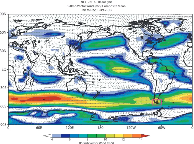
Figure 1. Global map showing the average wind (annual mean) at 850 mb during the period 1949-2013. The arrows indicate the prevalent wind direction, and the background colors the wind speed (m/s) (Image provided by the NOAA/
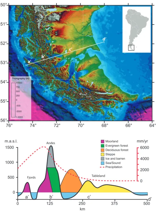
ESRL Physical Sciences Division, http://www.esrl.noaa.gov/psd). The Southern Patagonia territories (50°-56°S) are indicated by the purple color square. . . . . 3 Figure 2. (Above) Topographic map based on a digital elevation model (SRTM, 30 arc-
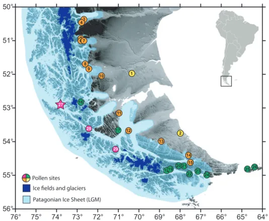
sec resolution; 90m) of Southern Patagonia territories (50°-56°S) and, (Below) schematic transect along the west-east axis (white line on the upper figure) denoting the precipitation gradient and the succession of main plant communities. . . . 4 Figure 3. Map of Southern Patagonia showing the location of pollen records (Table 1) and the
likely extension of the Patagonian Ice Sheet during the Last Glacial Maximum (LGM). The colour for each pollen site regards to the main vegetation occurring in the study area after the Figure 2. The star indicates the pollen record studied in this thesis (Tamar Lake). . . . 5 Figure 4. Geological map of southern Patagonia (after SERNAGEOMIN 2003, Ghiglione
et al. 2009; Fosdick et al. 2011) and inferred glacial limits during the LGM (after McCulloch et al. 2005; Coronato et al. 2008; Kaplan et al. 2008; Sagredo et al.
2011; Garcia et al. 2012). . . .10 Figure 5. Composite means for the period 1949-2013 illustrating the annual and seasonal
(winter and summer) patterns of zonal wind speed (above) and Sea Level Pressures (middle) occurring in the Southern Hemisphere, and its repercussions in the precipitation patterns along southern South America (below). The images were produced utilizing the online data provided by the NOAA/ESRL Physical Sciences Division, Boulder Colorado (http://www.esrl.noaa.gov/psd/). . . . . .12 Figure 6. Composite means for the period 1949-2013 illustrating the annual and seasonal
(winter and summer) temperatures of the air (above) and surface (below) in the southern South America. The images were produced utilizing the online data provided by the NOAA/ESRL Physical Sciences Division, Boulder Colorado (http://www.esrl.noaa.gov/psd/). . . . .13 Figure 7. Digital Elevation Model (DEM) and location of weather stations present in the
study area (53°S). Please note the under-represent values occurring during the winter months (MJJ) in the weather station of Gran Campo because the solid precipitation (snow). . . . .15 Figure 8. General map of Southern Patagonia, indicating the main plant formations occurring
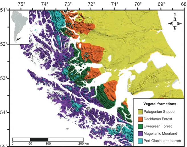
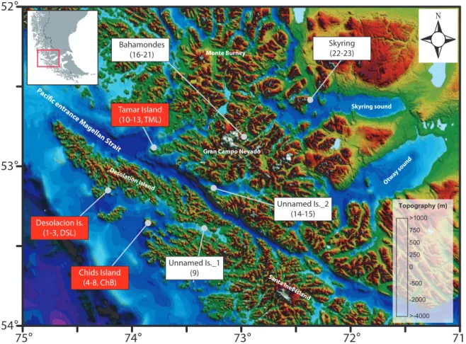
at regional-scale (after Schmithüsen 1956 and Gajardo 1994). . . . .17 Figure 9. Map of the study area (Southwest Patagonian Fjords, at 53°S) indicating the localities
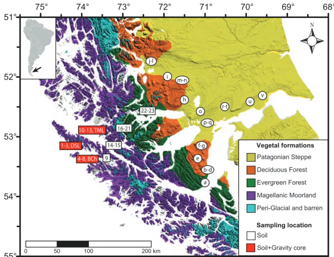
visited (n=7) where vegetation surveys and soil sampling were performed for the study of modern pollen-rain. The information into the rectangles refers to the name of the site and code for the samples retrieved (parenthesis) after Table 2. Rectangles in red indicate locations where additional samples from surface sediments (two lakes and one bay) were obtained. More details in the text. . . .19 Figure 10. Vegetation map (after Figure 8) showing the location of samples utilized to
the study of the modern pollen-rain that include the main plant formations
occurring along a west-east transect in Southern Patagonia. The information into
vii
the rectangles (this thesis) and circles (previous studies) indicates the codes of the samples provided in the Tables 2 & 3. . . .20 Figure 11. (A) General map of the Southwest Patagonian territories at 53°S (left) indicating
the location of the study site at Tamar Island (right). The yellow area in the georeferenced orthophoto denotes the lake catchment. (B) Oblique view (orthophoto+DEM) of the Tamar Lake catchment and elevation contour lines.
(C) Bathymetry map of Tamar Lake (left) indicating the location of the piston core (circle) and the performed echosounder tracks. The bold line denotes the track of the seismic profile plotted on the right. . . .26 Figure 12. Modern vegetation map (after figure 8) where is indicated the location of
pollen sites (rectangles) utilized to (i) examine changes in the plant community composition (turnover and richness) along a west-east gradient (at 53°S) and (ii) develop quantitative climatic reconstructions (transfer functions, see appendix section 8.2) for the postglacial. Locations for modern surface samples (pollen- rain) are also indicated. For more details see the text. . . . .30 Figure 13. Pollen diagram (relative percentage) from soil samples used to characterize
the pollen rain of the dominant plant communities occurring in Southwest Patagonia. Samples are grouped according to main vegetal formations and altitude. In addition, surface sediment samples (gravity cores) from Lake Tamar, Lake Desolacion and Chids Bay are included at the end. The locations of the study sites are indicated in the Table 2 and Figure 9. Black points indicates values
<5%. . . . .33 Figure 14. Cluster analysis (Edward & Cavalli-Sforza’s chord distance method) of the modern
pollen spectra from the Southern Patagonian Fjords. The analysis was performed using the samples obtained from soils and surface sediment (gravity cores). The name and colours indicates the main plant communities previously discussed (Figure 13). Grey rectangles indicate outliers. Sample codes are in parenthesis (Table 2). . . . .35 Figure 15. Principal Component Analysis for the main pollen types (>2%) on the first two
axes, using the samples obtained from soils and surface sediment (gravity cores) from the Southern Patagonian Fjords. . . .36 Figure 16. Pollen diagram (relative percentage) from surface samples used to characterize the
west-to-east modern pollen-rain along a broad biogeographic gradient (Figure 10 & Table 2). Colors indicate main groups defined by means of cluster analysis.
Black points indicates values <5%. . . . .38 Figure 17. Principal Component Analysis (PCA) for the main pollen types (>2%) present on
surface samples used to characterize the west-to-east modern pollen-rain along a broad biogeographic gradient (Figure 10 & Table 2). Colors indicate main groups defined previously by means of cluster analysis (Figure 16). . . . .41 Figure 18. Biplot showing the first two axes of the RDA ordination for modern surface
samples and selected taxa. Significant climatic variables Pann and Tann are denoted in red. Correlation and probability values are in the Table 6 . . . .42 Figure 19. Main physic features (elevation, aspect and slope) from the Tamar Lake
catchment . . . .43
Figure 20. Maps of the most relevant physical features occurring within of Lake Tamar
viii
catchment: A) elevation, B) aspect, and C) gradient slope. Below (D), vegetation mapping of Tamar Lake catchment. The images positioned left and right, represent the aerial and 3D perspective (respectively) view for each categorized maps. . . . .45 Figure 21. Composite image of the sediment core TML, showing: the position of radiocarbon
dates, a descriptive lithology column and the lithological sections discussed in the text, including the position of the different types of light-colored deposits (LCD’s). In the right are show the parameters of magnetic susceptibility and gray scale intensity . . . .48 Figure 22. Grayscale, magnetic susceptibility, and geochemical data from core TML1 versus
composite core depth (cm) and age (cal. yr BP). Color bars blue, red and green denotes the stratigraphic position of light-colored deposits (LCDs) Types 1-3 (respectively), while grey bars mark the two tephras originating from eruptions of Mt.-Burney. Red diamonds not line-connected on the geochemical parameters, indicates data points retrieved from LCDs. . . . .49 Figure 23. Age-depth model and sedimentation rates (mm yr
-1) for the composite sediment
core TML. The reliability of the model is constrained to the core sections were organic pelagic sedimentation occurs (lithological section II-IV). Note that the model is plotted against a corrected depth (without light-colored deposits and tephras layers). For more details see the text . . . .50 Figure 24. Close-up sections for the four different types of light-colored deposit (LCD’s)
present in the composite sediment core TML, indicating: length (cm), lithology, and the outcome of the parameters of grayscale and magnetic susceptibility for each one of them. . . .53 Figure 25. Chronology, thickness and frequency (per 1000 years) of events, based on
individualized light-colored deposits (LCD’s), present in the TML sedimentary record. Taking into account the differences observed among the LCD’s (e.g.
internal structure and distribution along the core), in the graph above (A) are plotted only the events corresponding to LCD’s types 1-3, while in the graph below (B) are plotted the events associated to the LCD’s type 4. Arrows in the graph B indicate periods when the recurrence among events is <100 years (sub- centennial time scales). . . . .55 Figure 26. Percentage diagram of selected taxa from Core TML, plotted against the calibrated
calendar age. The secondary y-axis displays the composite depth scale (cm).
Dashed lines represent the boundaries of pollen zones after the cluster analyses (CONNIS) in the right. Gray area (outside the curves) indicates a exaggeration factor x5. . . . .59 Figure 27. Concentration diagram (grains/cc) of selected taxa from the pollen record of Tamar
Lake. On the right of the graph are included the total concentration of terrestrial plants, ferns and aquatics. Please note the differences in the concentration scale among the taxa. . . .60 Figure 28. (Above) Biplot of Principal Component Analysis (PCA) for the pollen record
TML, performed on a re-calculated dataset containing only taxa >5%. The
respective pollen zone for each sample is indicated. (Below) Sample scores for
the Axis 1 and 2, plotted against age. Pollen zones are also indicated. Results
for the DCCA (Turnover) and the palynological rarefaction analysis (Richness)
ix
performed on the pollen record. The estimated palynological richness is based on the minimum number of pollen taxa (Tn). In order to highlight the major trends in the palynological turnover and richness, a Loess smoother (solid lines) has been fitted to the raw data, utilizing a sampling span of 1.5 and rejecting the outliers. . . . .62 Figure 29. (Above) Biplot of Principal Component Analysis (PCA) for the pollen record
GCN, performed on a re-calculated dataset containing only taxa >5%. The respective pollen zone for each sample is indicated. (Below) Sample scores for the Axis 1 and 2, plotted against age. Pollen zones are also indicated. Results for the DCCA (Turnover) and the palynological rarefaction analysis (Richness) performed on the pollen record. The estimated palynological richness is based on the minimum number of pollen taxa (Tn). The results are plotted against age. Pollen zones are indicated on the middle of the graph. In order to highlight the major trends in the palynological turnover and richness, a Loess smoother (solid lines) has been fitted to the raw data, utilizing a sampling span of 1.5 and rejecting the outliers. . . . .65 Figure 30. (Above) Biplot of Principal Component Analysis (PCA) for the pollen record
Rio Rubens, performed on a re-calculated dataset containing only taxa >5%.
The respective pollen zone for each sample is indicated. (Below) Sample scores for the Axis 1 and 2, plotted against age. Pollen zones are also indicated. Results for the DCCA (Turnover) and the palynological rarefaction analysis (Richness) performed on the pollen record. The estimated palynological richness is based on the minimum number of pollen taxa (Tn). The results are plotted against age. Pollen zones are indicated on the middle of the graph. In order to highlight the major trends in the palynological turnover and richness, a Loess smoother (solid lines) has been fitted to the raw data, utilizing a sampling span of 1.5 and rejecting the outliers. . . . .67 Figure 31. (Above) Biplot of Principal Component Analysis for the pollen record Laguna
Guanaco, performed on a re-calculated dataset containing only taxa >5%. The respective pollen zone for each sample is indicated. (Below) Sample scores for the Axis 1 and 2, plotted against age. Pollen zones are also indicated. Results for the DCCA (Turnover) and the palynological rarefaction analysis (Richness) performed on the pollen record. The estimated palynological richness is based on the minimum number of pollen taxa (Tn). The results are plotted against age. Pollen zones are indicated on the middle of the graph. In order to highlight the major trends in the palynological turnover and richness, a Loess smoother (solid lines) has been fitted to the raw data, utilizing a sampling span of 1.5 and rejecting the outliers . . . .69 Figure 32. (Above) Biplot of Principal Component Analysis for the pollen record Potrok Aike,
performed on a re-calculated dataset containing only taxa >5%. The respective
pollen zone for each sample is indicated. (Below) Sample scores for the Axis 1
and 2, plotted against age. Pollen zones are also indicated. Results for the DCCA
(Turnover) and the palynological rarefaction analysis (Richness) performed on
the pollen record. The estimated palynological richness is based on the minimum
number of pollen taxa (Tn). The results are plotted against age. Pollen zones are
indicated on the middle of the graph. In order to highlight the major trends in
the palynological turnover and richness, a Loess smoother (solid lines) has been
fitted to the raw data, utilizing a sampling span of 1.5 and rejecting the outliers. 71
x
Figure 33. Schematic profile indicating the distribution of main plant communities identified and described in this thesis, as the most characteristic in the Southern Patagonia Fjords (53°S). For each plant community the most representative taxa is indicated, while rare taxa are marked with a “+”. Main characteristics of the physical environment where each plant community occurs are also indicated on the left upper corner of the figure. . . .76 Figure 34. Images from Sub-alpine environments present in the Southern Patagonian Fjords
at 53°S. Left. General view of the vegetal landscape at ~300 m.a.s.l. Right. Detail of regolith formation in a wind exposed area at ~350 m.a.s.l. The red dashed line indicates the approximate elevation where sub-alpine environments take place.
Both photographs from Chids Island (for location see figure 9) . . . .77 Figure 35. Above. Analysis of the correlation between elevation and slope parameters for
two studied locations, Tamar Island and Chids Island (for location see Figure 9).
The analysis was performed using GIS, utilizing a grid of 100 m extracted from a DEM (SRTM, 3 arc-sec resolution; 90m). The red line represents the linear regression, and the blue the best fit-curve (quadratic). The yellow bar indicates the mid-elevations. Below. Basic conceptual diagram indicating the main stages and mechanisms involved in the transition from soil-mantled landscapes to bedrock-dominated landscapes in the Southern Patagonian Fjords. For details see text. . . . .79 Figure 36. Observed geomorphological context where forest communities occurs in the
visited areas on the Southern Patagonian Fjords . . . .80 Figure 37. Process of natural destruction of cushion-bogs observed in the visited areas. . . .80 Figure 38. Above. Comparison between summary pollen diagram (left) and PCA Axis 1
(right) from the modern pollen-rain samples retrieved in the Fjords and vicinity areas. Below. Boxplots for percentages corresponding to the different plant communities identified and studied, and linear regression between PCA Axis 1 and soil cover classes. The box encloses the middle half of the data between the first and third quartiles. The central line denotes the value of the median. The horizontal line extending from the top and bottom of the box indicates the range of typical data values. Outliers are displayed as “o” for outside values and “*” for far outside values . . . .83 Figure 39. Left. Comparison between summary pollen diagram, PCA Axis 1 and cluster
analyses. Right. Boxplots of percentages for the main plant formations studied in this thesis located along the west-east transect. The box encloses the middle half of the data between the first and third quartiles. The central line denotes the value of the median. The horizontal line extending from the top and bottom of the box indicates the range of typical data values. Outliers are displayed as “o” for outside values and “*” for far outside values . . . .86 Figure 40. Map of the study area at 53°S indicating the locations of paleoenvironmental
proxies discussed in the text. The star shows the location of Tamar Island and TML core. Glaciers are marked in orange and inferred ice limits in yellow.
Minimum ages corresponding to ice retreat are also provided. . . .89 Figure 41. Summary figure for main geochemical and palynological results from the TML
core, and selected paleoclimatic proxies . . . .90
xi
Figure 42. Left. View of the Lake Tamar catchment and surrounding vegetation. Lake bathymetry and lithology of gravity cores are shown . . . .93 Figure 43. Summary figure of main abiotic and biotic proxies from the TML core . . . . .96 Figure 44. Summary figure for abiotic (geochemical) and biotic (pollen) from TML and
selected paleoclimatic proxies. For location see figure 40 . . . .97 Figure 45. Summarized pollen concentration diagram of tree taxa, indicating its shade
tolerance. The red arrow indicates the point when the taxon becomes abundant in the record. . . . .98 Figure 46. Comparison of the results obtained from the principal component analysis (PCA),
detrended canonical correspondence analysis (Turnover) and Rarefaction analysis (Richness) performed at the four additional pollen records located along the west-east transect in Southern Patagonia (Figure 12). In all the cases, the results are plotted against time. The data from Turnover and Richness were smoothed utilizing a 0.2 lowesss spline (solid line). The estimated palynological richness was calculated based on the minimum number of pollen taxa (Tn) at each site.
Also selected paleoclimatic proxies are provided. . . . . 101 Figure 47. Schematic evolution of the main vegetation types of Southern Patagonia during
the Postglacial. . . 102 Appendix figure 1. Co-occurrence network from the quantitative content analysis performed
on a dataset that include only scientific publications (n=29) related with Quaternary palynological issues of Southern Patagonia (see table 1 for references).
The results (co-occurrence networks) are representing words (nodes) from the texts (excluding the bibliography) from the analysed pollen publications-dataset.
Two methods and analysed in terms of: sentences (left) and paragraphs (right).
The resulting co-occurrence network was measured utilizing a community- modularity clustering method (Clauset et al. 2004). The position of the nodes was calculated use Fruchterman-Reingold algorithm (Fruchterman and Reingold) . 121 Appendix figure 2. Idealized wind behaviour scenarios in a landscape with and without
topography. Above. Cross section along the landscape in where is indicated with red lines the wind behaviour in a scenario without topography, and with blue lines the wind behaviour in the presence of a mountain (grey). Below.
Graph for wind speed versus height along three profiles (a,b,c). The first (a) characterizes the idealized behaviour of the wind speed along the height in the absence of topography. On the contrary the profiles a and b denotes the effect of the topography. Notice the increase of the flow (wind speeds) in response to the topography because the compression of the flux in the top of the hill, and the presence of a wind-sheltered zone on the leeward (Modified from several sources). . . 122 Appendix figure 3. (Above) Hanging vegetation occurring in coastal areas and, (Below) an
example of the observed absence of vegetation probably related to characteristics of rock type. . . . . 123 Appendix figure 4. Images showing the area affected by a recent landslide in the area of Bahia
Bahamondes, being appreciable the soil covered by Gunnera magellanica. . . . 124
Appendix figure 5. Panoramic view of Tamar lake, Chids bay and Desolacion lake. . . . . 125
xii
Appendix figure 6. Boxplots of modern pollen rain percentages for selected taxa arranged by dominant plant formations occurring in Southern Patagonia. The box encloses the middle half of the data between the first and third quartiles. The central line denotes the value of the median. The horizontal line extending from the top and bottom of the box indicates the range of typical data values. Outliers are displayed as “o” for outside values and “*” for far outside values. Note changes in scale. . . 126 Appendix figure 7. Detail of the magnetic susceptibility results from the Tamar lake sediment
core indicating in gray the basal section of the record where predominates clays (light gray) and sandy layers (dark gray). . . . . 127 Appendix figure 8. Boxplots of selected geochemical parameters for pelagic sediments (matrix)
and LCD’s (types 2-4) present within of the sediment core from Tamar lake . The box encloses the middle half of the data between the first and third quartiles. The central line denotes the value of the median. The vertical line extending from the top and bottom of the box indicates the range of typical data values. Outliers are displayed as “o”. . . 128 Appendix figure 9. Percentage diagram of the pollen record from Tamar of lake, where are
included the samples (in red) associated to mass wasting deposits or light-colored deposits (LCDs). Colour bars blue, red and green denotes the stratigraphic position of LCDs Types 1-3 (respectively). . . . . 129 Appendix figure 10. Plant macrorest found in the mass wasting deposits of Tamar lake
sediment core. . . . . 130 Appendix figure 11. Leaves of Nothofagus betuloides found in the mass wasting deposits of
Tamar lake sediment core. . . 131 Appendix figure 12. Concentration diagram (grains/cc) including all the taxa from the pollen
record of Tamar Lake. . . . 132 Appendix figure 13. Percentages pollen diagram from Gran Campo Nevado sediment core. 133 Appendix figure 14. Percentages pollen diagram from Rio Rubens sediment core. . . 134 Appendix figure 15. Percentages pollen diagram from Lago Guanaco sediment core. . . . 136 Appendix figure 16. Percentages pollen diagram from Potrok Aike sediment core. . . 137 Appendix figure 17. Scatter plot of the predicted precipitation values versus the observations
(upper panel) and its respective residuals (lower panel), for the WAPLS and MAT models . . . 141 Appendix figure 18. Boxplots of estimated precipitation (Pann) from the transfer function
models (MAT and WAPLS) for each of the pollen records utilized in this thesis in order to perform quantitative paleoprecipitation reconstructions along a west- east transect at ~53°S (Figure 12). The box encloses the middle half of the data between the first and third quartiles. The central line denotes the value of the median. The vertical line extending from the top and bottom of the box indicates the range of typical data values. Outliers are displayed as “o”. . . . 143 Appendix figure 19. (Left) Reconstructed annual precipitation (Pann) parameter from the
pollen record of Tamar lake, utilizing the transfer functions WAPLS (red) and
MAT (blue). The green arrow and dashed line indicate the modern Pann at the
xiii
study site. (Right) Results from a simple subtraction operation (expressed in mm) performed among the transfer functions, in order to visualize more easily divergences between the curves. The solid-hard line on the graphs correspond to a Loess smoother, have been fitted to the raw data in order to highlight the major trends, utilizing a sampling span of 1.5 and rejecting the outliers. . . 144 Appendix figure 20. (Left) Reconstructed annual precipitation (Pann) parameter from
the pollen record of GCN, utilizing the transfer functions WAPLS (red) and MAT (blue). The green arrow and dashed line indicate the modern Pann at the study site. (Right) Results from a simple subtraction operation (expressed in mm) performed among the transfer functions, in order to visualize more easily divergences between the curves. The solid-hard line on the graphs correspond to a Loess smoother, have been fitted to the raw data in order to highlight the major trends, utilizing a sampling span of 1.5 and rejecting the outliers. . . 145 Appendix figure 21. (Left) Reconstructed annual precipitation (Pann) parameter from the
pollen record of Rio Rubens, utilizing the transfer functions WAPLS (red) and MAT (blue). The green arrow and dashed line indicate the modern Pann at the study site. (Right) Results from a simple subtraction operation (expressed in mm) performed among the transfer functions, in order to visualize more easily divergences between the curves. The solid-hard line on the graphs correspond to a Loess smoother, have been fitted to the raw data in order to highlight the major trends, utilizing a sampling span of 1.5 and rejecting the outliers. . . 147 Appendix figure 22. (Left) Reconstructed annual precipitation (Pann) parameter from the
pollen record of Lago Guanaco, utilizing the transfer functions WAPLS (red) and MAT (blue). The green arrow and dashed line indicate the modern Pann at the study site. (Middle) Results from a simple subtraction operation (expressed in mm) performed among the transfer functions, in order to visualize more easily divergences between the curves. The solid-hard line on the graphs correspond to a Loess smoother, have been fitted to the raw data in order to highlight the major trends, utilizing a sampling span of 1.5 and rejecting the outliers. Notice that reconstructed annual precipitation (Pann) utilizing the MAT transfer functions is plotted as single graph in the right of the figure. . . 148 Appendix figure 23. (Left) Reconstructed annual precipitation (Pann) parameter from the
pollen record of Potrok Aike, utilizing the transfer functions WAPLS (red) and
MAT (blue). The green arrow and dashed line indicate the modern Pann at the
study site. (Right) Results from a simple subtraction operation (expressed in
mm) performed among the transfer functions, in order to visualize more easily
divergences between the curves. The solid-hard line on the graphs correspond to
a Loess smoother, have been fitted to the raw data in order to highlight the major
trends, utilizing a sampling span of 1.5 and rejecting the outliers. . . 150
xiv
List of Tables
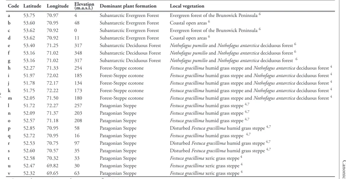
Table 1. Summary table indicating the code (number), name, location and altitude of palynological studies performed in Southern Patagonia (Figure 3). Note that sites are ordered according to the dominant plant formation present on each of the study sites. . . 9 Table 2. Codes and main geographical characteristics (coordinates/elevation, site name and
dominant plant formations) of the surface samples collected in this thesis to study the modern pollen-rain within the Southern Patagonian Fjords. . . . . .22 Table 3. Additional surface sample locations (Quintana 2009) utilized to develop a
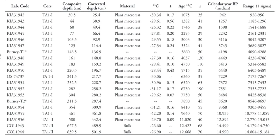
comprehensive study of the modern pollen-rain along a broad west-to-east transect in Southern Patagonia (53ºS). For more details see the text. . . . 24 Table 4. Radiocarbon dates for the Tamar Lake composite core, indicating corrected depths
after be subtracted all the layers related to events of instantaneous deposition (e.g.
tephra, mass flows). Radiocarbon samples have been calibrated using Calib 6.1.0 and the Southern Hemisphere calibration curve (SHCal04). For ages beyond the SHCal04 calibration curve were used the IntCal04 calibration curve. Median and 1 sigma of distribution for each calibrated radiocarbon date are provided.
The age of tephra layers are based on previously reported results (Kilian et al.
2003). For more details see the text. . . .28 Table 5. Climatic and geographic variables used in the ordination analysis (RDA). Variables
in bold are significant at p-value<0.005. . . .41 Table 6. Correlations and inter-correlations between significant climatic variables and RDA
axis. . . .42 Table 7. Total and relative areal cover of the main plant communities identified within the
Tamar Lake catchment, and the physical features characterizing the areas where they occur. . . .44 Table 8. Summary of principal component analysis (PCA) and detrended canonical
correspondence analyses (DCCA), measure of trends in turnover (beta- diversity), total inertia (total variance in each sequence), and the first eigenvalue (λ1) measure of the contribution of the first axis to total variance at the four study sites, using both all samples and only those samples covering the period in common (12,750 cal yr BP to present). . . .64 Table 9. Main ecological traits for tree taxa involved in the postglacial forest succession in the
Tamar pollen record . . . .99 Appendix table 1. Chronology of events associated to light-colored deposits (LCDs) present
in the sediment core of Tamar Lake . . . 138 Appendix table 2. Performance of the reconstruction models, indicating: the coefficient
of determination between predicted and observed climate values (R
2), the
maximum bias (Max. bias), root mean square error of prediction (RMSEP) and
the percentage of change among the components (%Change). The best model
within each set of algorithms are indicated in color, namely: MAT (Modern
analogue technique), WA (weighted averaging) and WAPLS (Weighted averaging
partial least squares regression). For more details see the text. . . . 141
xv
Appendix table 3. Basic statistic parameters for each of the reconstructions (WAPLS and MAT) performed on selected pollen records located along a west-east transect at
~53°S. . . 142
1
INTRODUCTION 1. INTRODUCTION
1.1. Background
The configuration of modern ecosystems, in terms of its distribution and composition, is the result of complexes processes tied inherently to particular environmental forcings in time (Delcourt et al. 1983, Delcourt and Delcourt 1988, Seppä and Bennett 2003, Willis and Birks 2006, Davies and Bunting 2010, Rull 2010, Willis et al. 2010, Vegas-Vilarrubia et al. 2011). Today it is broadly accepted that climate exerts a key control over the distribution of the world’s major ecosystems (Holdridge 1947, Whittaker 1975), and therefore past climate changes must have also been imprinted through changes in biota (Bennett 1997, Lieberman 2000)
1. A classic example which illustrates the role of climate as a key environmental forcing are the profuse and coeval changes observed in the distribution and composition of terrestrial and marine ecosystems (Coope and Wilkins 1994, Hewitt 2000, Willis et al. 2004, MacDonald et al. 2008) during the successive glacial-interglacial cycles which characterize the Quaternary (<2.6 Ma)(Pillans and Naishb 2004, Gibbard et al. 2009). Nevertheless, this apparent synchronicity and correlation between changes in climate and biota lessen in importance when the spatial-temporal scale decreases, giving way to a new level in which ecological factors acquire relevance (Delcourt et al. 1983, Delcourt and Delcourt 1988). In other words, environmental forcing functions and biotic responses vary according to the temporal and spatial scales investigated.
The palynology as a proxy for the study of past plant communities
Palynology or pollen analysis; the study of fossil pollen and spores, is the principal technique utilized to perform vegetational reconstructions at various timescales (Fægri and Iversen 1989).
Since its development by Von Post (Manten 1967), palynological studies have provided significant contributions to Quaternary sciences, being utilized largely as a paleoclimatic proxy
2. Nevertheless, even when climate strongly influences the geographical distribution of plants and vegetation types (Woodward 1987), the evidence also indicates that vegetation changes are not always in equilibrium with it (Webb 1986). For example, the observed time lag (~1500 yr) between climate change and postglacial spread of temperate trees in northern Europe has been interpreted as result of deficient soil development in areas previously covered by ice (Pennington 1986). In comparison, in areas not covered by ice during the last glacial maximum the process is reversed, beginning with the forest arrival and then the development and maturation of soils (Willis et al. 1997). Other examples illustrating the participation of non-climatic mechanisms in the reconstructed changes and patterns (e.g. succession) of the vegetation involve dispersal mechanisms (Wilkinson 1997), interspecific competition (Bennett and Lamb 1988), disturbance mediated by wildfires (Bond et al. 2005), pathogens attack (Waller 2013) and human activities (Edwards and MacDonald 1991).
In recent years, several studies have highlighted the relevance of including a long-term perspective for conservation strategies and policies (Willis and Birks 2006, Davies and Bunting 2010, Willis et al. 2010, Vegas-Vilarrubia et al. 2011, Birks 2012). In this context, palynological studies provide a robust tool to examine the biotic responses to environmental forcing (climatic and non-climatic) along different spatial-temporal scales. Paleoenvironmental information inferred from pollen records is not solely restricted to vegetation reconstructions. Nowadays, owing to the
1 The notion of climate as the main control in the distribution of global biota, was first mentioned in the 18th century by Carl Linnaeus “On the increase of the habitable Earth” (Oratio de Telluris habitabilis incremento, 1744). Nevertheless, it was only during the 19th century when the idea of climate changes conducing changes on the biota with time was conceived. This invaluable contribution to the science is discussed of two classic works of the epoch:: “Principles of Geology (1837)” of Charles Lyell “and “The origin of the species (1859)” of Charles Darwin.
2 For more details refer to section: Pollen records, in the Encyclopedia of Quaternary Science (Brewer et al. 2007).
2
Background development of new statistical tools and numerical analysis, it is possible to estimate qualitative changes in the diversity and composition of the ecosystems on various scales (Odgaard 2007)
3. Consequently, ecological thresholds and resilience
4of plant communities to environmental forcing over different timescales can be examined (Birks and Birks 1980, Delcourt et al. 1983, Prentice 1986, Delcourt and Delcourt 1988, Delcourt and Delcourt 1991, MacDonald and Edwards 1991, Huntley 1996, Seppä and Bennett 2003, Rull 2010, Willis et al. 2010, Birks 2012).
Rationale: Southern Patagonia as a case study
Southern Patagonia (50°-56°S) is key region for paleoenvironmental studies addressing complex paleoclimatic and paleoecological questions, due to a number of physical and biotic singularities that characterize local environments. Firstly, Southern Patagonia located at the tip of South America is the only continental landmass extending south of 38°S (Australia) and the most austral continuous land south of 46°S (New Zealand; Figure 1)
5. The absence of significant landmasses in mid and high latitudes of the Southern Hemisphere, allows the development of a symmetric behaviour in the flux of the Southern Westerly Wind belt (SWW), a key component of the coupled atmosphere-ocean system (Garreaud et al. 2009)(Figure 1). Several studies have highlighted the importance of examining the dynamics of the SWW (e.g. strength and position) through time, due to its influence on climate of mid-high latitudes of the Southern Hemisphere.
The SWW are linked with the global climate due to its role in the active upwelling mechanism of deeper Antarctic Circumpolar Current (ACC) waters and the subsequent repercussions for CO
2degassing from the Southern Ocean (Thompson and Solomon 2002, Shulmeister et al. 2004, Varma et al. 2012, Razik et al. 2013). Therefore, the Southern Patagonia territories are a key location for undertaking paleoenvironmental studies to reconstruct and examine changes in the dynamic of the SWW at various timescales.
A further noteworthy characteristic of the Southern Patagonia territories is the succession of distinct biophysical environments along the west-east axis (Figure 2). This feature, result of million of years of tectonic history and evolution of biota
6, can be summarized to: (i) a main cordillera dividing dissimilar landscapes occurring in the west (Fjords) and the east (plains and tablelands), (ii) creating a strong orographic precipitation gradient along the west-east axis, and with (iii) the consequent occurrence of hyper-humid climates in the west and semi-desert in the east (Endlicher and Santana 1988, Schneider et al. 2003, Coronato et al. 2008, Garreaud et al. 2013)(Figure 2). The vegetation follows this natural west-east gradient, with the dominance of Moorlands ecosystems in the western Fjords, Evergreen and Deciduous Forest in the Andean region, and extensive grasslands ecosystems (Steppe) along the eastern plains(Schmithüsen 1956, Oberdorfer 1960, Pisano 1977, Boelcke et al. 1985, Gajardo 1994)(Figure 2).
3 Whittaker et al. (2001) offers a coherent discussion about changes in the species diversity along different spatial-temporal scales, propos- ing a hierarchical schema that distinguishes five main diversity tiers: community (α-diversity), between-community (β-diversity), landscape (γ-diversity), between-landscape (δ-diversity), and regional (ε-diversity).
4 The ecological threshold refers to the point at which there is an abrupt change in the properties or structures of an ecosystem, whereas the ecological resilience regards with the ability of the (eco)systems to tolerate disturbances (i.e environmental forcings) and still maintain the properties or structures similar to the pre-disturbance state (for more details see Groffman et al. 2006).
5 This observation excludes the Antarctic territories and the subantarctic islands (Auckland, Kerguelen, Falkland and South Georgia, among others).
6 Geologic and paleobotanic information suggest that the first stages of the differentiation between the biogeographic subregions of Subantarc- tic (west) and Patagonia (east), are closely related with the progressive uplift of Patagonian Andean Cordillera during the Late Miocene (14-10 Ma) and the Early Pliocene (5 Ma), and the subsequent develop of the rain-shadow effect (Hinojosa and Villagrán 1997; Villagrán and Hinojosa 2005; Ortiz-Jaureguizar and Cladera 2006). Thereby, these antecedents highlight the ancient roots of the physical and environmental gradient studied in this thesis..
3
Background
Several paleoenvironmental studies have been conducted within this biophysical gradient, using different kinds of archives and proxies (Kilian and Lamy 2012). The findings, which indicate significant changes in the biotic and abiotic components of the reconstructed paleoenvironments, suggest important transformations in the ecosystems under the action of environmental forcing.
Pollen studies, the most common paleoenvironmental proxy utilized in Southern Patagonia (Kilian and Lamy 2012), have been largely used to reconstruct past climate changes and specifically changes in the SWW dynamic, but hardly to address paleoecological questions (Appendix figure 1)
7. For example, a well-know feature observed in all pollen records is the increase of tree pollen percentages during the postglacial, denoting the spread of forest communities through the region (Markgraf 1993, McCulloch and Davies 2001, Mancini 2002, Heusser 2003, Fesq-Martin et al. 2004, Huber et al. 2004, Villa-Martinez and Moreno 2007, Mancini 2009, Wille and Schäbitz 2009, Markgraf
7 As a direct way to exemplify the observed lack of non-climatic topics in the main discussions of palynological studies, a quantitative text analysis content was performed over a dataset that included all palynological publications published until present. The analysis was performed using co-occurrence networks, a common statistical technique utilized in quantitative content analysis to determine the presence of certain words, concepts, themes, phrases, characters, or sentences within texts or sets of texts and to quantify this presence in an objective manner (Danowski 1993). In this case, the co-occurrence network approach was used to identify the main focus or trends, and the correlations among concepts. The results highlighted the lack paleoecological topics in the text, and the strong correlation among the concepts pollen-record and climate. More information is provided in the appendix section (Appendix figure 1).
NCEP/NCAR Reanalysis 850mb Vector Wind (m/s) Composite Mean
Jan to Dec: 1949-2013
850mb Vector Wind (m/s)
4 6 8 10 12 14
NOAA/ESRL Physical Sciences Division
90N
60N
EQ
30S
60S
90S 30N
0 60E 120E 180 120W 60W 0
Figure 1. Global map showing the average wind (annual mean) at 850 mb during the period 1949-2013. The arrows
indicate the prevalent wind direction, and the background colors the wind speed (m/s) (Image provided by the NOAA/
ESRL Physical Sciences Division, http://www.esrl.noaa.gov/psd). The Southern Patagonia territories (50°-56°S) are
indicated by the purple color square.
4
Background and Huber 2010, Moreno et al. 2010, Ponce et al. 2011). The timing and structure of this change is site-dependent, suggesting a complex history in forest expansion and establishment through the region during the postglacial. Absence of dispersal agents, insufficient soil development, intra- and interspecific competition, and/or features related with the distance from refugial areas and physical barriers in the routes of migration, are some of the plausible factors able to modify the dynamic of colonization and spread of tree taxa (Giesecke 2007). However, in most palynological studies interpret these changes are interpreted only in terms of precipitation changes associated with the SWW dynamics.
51°
50°
76° 74° 72° 70° 68° 66° 64°
56°
55°
54°
53°
52°
0
>1000 500
>-4000 -2000 -500 250 750 Topography (m)
a’ b’
c’
d’
375 1500
1000
500
0
0 125 250
km
500 m.a.s.l.
a’ d’
Fjords
Andes
Tableland
b’ c’
0 2000 4000 6000 mm/yr
Moorland Evergreen forest Deciduous forest Steppe Ice and barren Sea/Sound Precipitation
Figure 2. (Above) Topographic map based on a digital elevation model (SRTM, 30 arc-sec resolution; 90m) of
Southern Patagonia territories (50°-56°S) and, (Below) schematic transect along the west-east axis (white line on the
upper figure) denoting the precipitation gradient and the succession of main plant communities.
5
Background Additionally, it is important to mention the anomalous conglomeration of pollen records along the Andes and adjacent territories, and the resulting low representation of the steppe and moorland environments in paleoenvironmental studies (Figure 3). This is partly due to the lack of suitable locations to acquire paleoenvironmental records in the east (due to the prevalent dry climatic conditions) and due to logistic difficulties in accessing western locations
8(Kilian and Lamy 2012). The lack of data in the west (i.e. Channels and Fjords) is can be also seen in the sparse vegetation surveys (Luebert and Pliscoff 2006) undertaken and the absence of pollen-rain studies (Schäbitz et al. 2013) both prerequisites for the interpretation of pollen records (Fægri and Iversen 1989).
In light of the above, this study aims to investigate these ecological issues such as the actual distribution and composition of main plant communities occurring in Western Patagonia, as well as the representation of these plant communities in the modern pollen rain. The relationships between pollen assemblages (i.e. vegetation types) and key environmental variables (i.e. climate, altitude, etc) have been not studied by previous studies concerning the modern pollen-rain (Mancini 1998, Prieto et al. 1998, Heusser 2003, Trivi et al. 2006, Mancini et al. 2012). Hence, with the development of a modern pollen-rain study in the fjords is possible solve the sampling bias exhibited by previous studies, and to perform quantitative analyses to explore the relationship between pollen assemblages and environmental variables along a range which includes all the main plant formations from Southern Patagonia (Figure 2).
8 The Southern Patagonian Fjords are one of the most isolated and unpopulated areas in southernmost South America (estimated demographic density <0.01 inhabitant/km2, source INE). This explains why its territories, at present, contain several pristine ecosystems, making some areas of the western Andes particularly important in terms of conservation (Martínez-Harms and Gajardo 2008).
53°
52°
51°
50°
76° 75° 74° 73° 72° 71° 70° 69° 68° 67° 66° 65° 64°
56°
55°
54°
Patagonian Ice Sheet (LGM) Ice fields and glaciers Pollen sites
3
5 4
6 7
89
10 1
12 11
17
13 2
14 16
18 2115
22 23 24 25 26
29
19 20 28
27
Figure 3. Map of Southern Patagonia showing the location of pollen records (Table 1) and the likely extension of the