Research
The software maintenance
project effort estimation model based on function points
Yunsik Ahn∗,†, Jungseok Suh, Seungryeol Kim and Hyunsoo Kim
Kyungwon College, Sungnam, Kyungki-Do, Seoul, Korea
SUMMARY
In this study, software maintenance size is discussed and the software maintenance project effort estimation model (SMPEEM) is proposed. The SMPEEM uses function points to calculate the volume of the maintenance function. Ten value adjustment factors (VAF) are considered and grouped into three categories of maintenance characteristics, that is the engineer’s skill (people domain), its technical characteristics (product domain) and the maintenance environment (process domain). Finally, we suggest an exponential function model which can show the relationships among the maintenance efforts, maintenance environment factors, and function points of the software maintenance project. Regression analysis of some small maintenance projects demonstrates the significance of the SMPEEM model. Copyright c2003 John Wiley
& Sons, Ltd.
KEY WORDS: function point; software maintenance; maintenance project effort estimation
1. INTRODUCTION
Software maintenance is categorized into adaptive, corrective, preventive and perfective [1–3]. Most organizations are concerned about the costs of software maintenance, for it has been increasing steadily and many companies spend approximately 80% of their software budget on maintenance [4,5].
Therefore, these organizations need to manage their software maintenance efforts and costs effectively.
However, there are fewer effort estimation models for a software maintenance project compared with software development.
∗Correspondence to: Yunsik Ahn, Kyungwon College, Mt. 65 Bokjeong-Dong Sujeong-Gu, Sungnam, Kyungki-Do, Seoul, Korea 461-701.
†E-mail: ysahn@kwc.ac.kr
The major issues in estimation related to software maintenance efforts include the software system’s size and maintenance productivity [4]. A number of estimation models for software development have been broadly adopted such as size measures as source lines of code, function points, etc. [6]. Lines of code (LOC) have also been adopted as the size measure of software maintenance in spite of some difficulties which derived from the variation in the definition on source codes itself and counting the new, changed, or reused lines delivered. However, counting the LOC for a prioriestimation is usually difficult in order to estimate how much effort would be required for software maintenance [6,7]. In addition, productivity factors on software maintenance projects should be differentiated from those for software development projects.
In this study, the software maintenance project effort estimation model (SMPEEM) is proposed which is based on the function point measure and new maintenance productivity factors. The SMPEEM is empirically validated focusing on small maintenance projects.
2. LITERATURE REVIEW
In this section, some models related to the estimation of maintenance efforts and productivity of software maintenance are reviewed.
2.1. Estimation model for software maintenance efforts
There are some sizing approaches for estimating the software maintenance efforts such as source lines of code (SLOC) [8], function points (FPs) [9], and object points [10,11]. We review the annual change traffic (ACT) model, the FP model and COnstruction COst MOdel (COCOMO) 2.0 reuse model.
The ACT model estimates the maintenance size depending on the actual data of annual change traffic and the FP model counts the number of FPs. The COCOMO 2.0 reuse model reflects the estimated efforts for modifying reusable software. Each model is described in detail.
2.1.1. The ACT model
ACT is defined as ‘the fraction of the software product’s source instructions which undergo change during a typical year, either addition or modification’ [12]. Boehm established Equation (1) for estimating maintenance costs using the data gathered from 63 projects [13]
AME=ACT×SDT (1)
where AME and SDT are the annual maintenance effort and the software development time, respectively. The dimension of AME may be expressed in man-months (MM). Similarly, Schaefer’s study suggests the following Equation (2) [14]:
E=ACT×2.4KLOC1.05 (2)
whereEis the effort (MM) required to maintain the software annually. ACT is defined as the ratio of the system undergoing maintenance and the number of source code instructions that are modified or added during one year of maintenance.
These models are derived from the original COCOMO model. They are mainly applicable for annual maintenance cost estimation where an organization has the historical data for ACT. Therefore, the following fundamental problems are still present in these models.
First, if the systems are completely new and there is no historic basis for estimating the ACT, the results of estimation are likely to be unreliable. Second, the quantity of source code changed and added does not always represent the effort of the maintenance project. Third, expressing software size using lines of codea priorito the project can vary. Finally, this approach has the critical risk that it does not consider quantitatively any scientific attributes representative of software maintainability.
An estimation guide [15] of software maintenance costs may be calculated as the multiplication of the system’s LOC and maintenance adjustment score. Five factors, such as the frequency of required maintenance, the volume of processed data, the relevance of the external system, the necessity of understanding business rules, and the degree of distributed processing are checked for their maintenance adjustment score [15]. However, this model also contains the insufficiencies of the ACT model, because the maintenance workload is computed as LOC and the frequency of required maintenance is considered as a kind of ACT which cannot be easily estimated.
2.1.2. The COCOMO 2.0 reuse model
The COCOMO 2.0 model is an update of the COCOMO model [16]. The post-architecture stage of this model has the following form:
Effort=A× [size]1.01+5i=1SFi × 17 i=1
EMi (3)
whereAis a constant and the size is measured in terms of KSLOC (thousands of source lines of code), FPs or object points. SF means the five scale factors such as precedentedness, development flexibility, architecture/risk resolution, team cohesion and process maturity. EM means the 17 effort multipliers including the required software reliability, database size, product complexity, required reusability, documentation, etc.
In the viewpoint of the software maintenance project, the size and instructions of a new project (SLOC), are derived from the following equation:
SLOC=ASLOC×(AA+SU+0.4×DM+0.3×CM+0.3×IM)
100 (4)
In Equation (4), the size involves the estimated amount of software to be adapted (ASLOC), the rating scale for assessment and assimilation increment (AA), the software understanding increment (SU), and three degrees of modification parameters: DM, the percentage of design modification; CM, the percentage of code modification; and IM, the percentage of the original integration effort required for integrating the reused software. The rating scale for AA has five levels relating to the effort of module test and evaluation (T&E) and documentation. As for SU, the rating scales are decided by the degree of the software’s structure, applications clarity, and self-descriptiveness factor.
We can, however, consider this model as a management model rather than an estimation model, because of the modification parameters which cannot be estimated before the planning stage of the maintenance project.
2.1.3. The FP model
The FP model [17] was developed originally for the effort estimation of a new software project in the 1970s and was expanded to the software maintenance and enhancement project by Albrecht’s FP revision model [18].
The FP model defines the five basic function types to estimate the size of the software. Two data functions types are internal logical files (ILF) and external interface files (EIF), and the remaining three transactional function types are external inputs (EI), external outputs (EO), and external inquiries (EQ).
In order to adopt this FP model, the maintenance and enhancement project function point calculation consists of three components of functionality [9]: (1) the application functionality which is included in the user requirements for the project; (2) the conversion functionality; and (3) the value adjustment factor (VAF).
Application functionality consists of FPs which are added, changed, and deleted by a maintenance project. Conversion functionality consists of FPs delivered because of a conversion. The VAF is based on the 14 weighted characteristics. The degree of influence ranges from zero to five, from no influence to strong influence.
The formula for the maintenance and enhancement project FP calculation is defined as follows [9]
EFP=(ADD+CHG+CFP)×VAFa+(DEL×VAFb) (5)
where EFP is the enhancement project function point, added (ADD), changed (CHG), deleted (DEL) FPs are counted as application functionality, and CFP means the unadjusted function points added by conversion. VAFa and VAFb are the value adjustment factor of the application after and before the project, respectively.
Function point counts are a more consistenta priorimeasure of software size compared to the source lines of code [6]. FP is currently the functional size metric most often used and it continues to gain adherents in the management information system field and has proven to be successful for building productivity models and for estimating project costs [19].
However, the VAF of this model is originally introduced for a new software development project.
There are several examples of VAFs such as data communications, distributed processing, and performance, etc. These factors are not also applicable to the maintenance environment and cannot be measured with an objective view.
2.2. Productivity factors on software maintenance
In general, maintenance costs are difficult to estimate, because these costs are related to the number of product, process, and organizational factors related to the productivity of software maintenance.
Some models do not differentiate the productivity factors of software maintenance from those of development [9,20]. However, the productivity factors of software maintenance differ from those of software development.
The major maintenance cost driver is associated with the size, age, and complexity [21]. Sommerville [2] asserted that the productivity factors concerning the environment of software maintenance can include characteristics such as module independence, programming language, programming style etc.
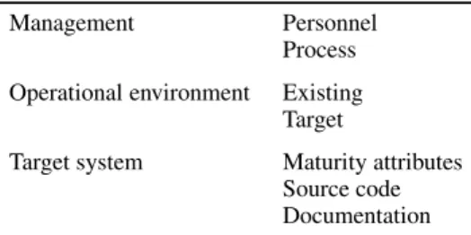
Table I. Software maintainability hierarchy.
Management Personnel
Process Operational environment Existing
Target
Target system Maturity attributes Source code Documentation
In 1985, software productivity research (SPR) introduced a new way to calculate function points [22]. The SPR technique for dealing with complexity is to separate the overall complexity into three distinct areas: problem complexity, code complexity, and data complexity. In this way, the effort to complete the calculations can also be reduced. Also, software maintainability characteristics were expressed as a hierarchical structure of seven attributes by Oman’s research as shown in TableI[23].
Beladyet al.consider maintenance efforts as the aforementioned productivity effort, complexity of software design and documentation, and the degree of familiarity with the software [24]. Jorgensen’s effort prediction model includes variables such as the cause of the task, the degree of change in the code, the type of operation on the code (mode), and the confidence of the maintainer [25]. The questionnaires in the study asked for information of environmental characteristics including technical constraints (response time, security, number of users, platforms), maintenance tools and techniques (development methodology, CASE tools), and factors related to personnel (number of programmers, experience) [3].
In the perspectives of software product, the size of both the software understanding and the module interface checking penalty can be reduced by good software structuring [16], because modular and hierarchical structuring can reduce the number of interfaces which need checking (discussed in [16]).
Therefore, the various characteristics which have an influence on software maintenance productivity should be refined.
3. SOFTWARE MAINTENANCE PROJECT EFFORT ESTIMATION MODEL
This section provides a description of the suggested Software Maintenance Project Effort Estimation Model (SMPEEM). After introducing the approach, the process of counting and adjusting the function points is explained. Finally, the adjusted function points are applied to estimate the software maintenance effort by using SMPEEM.
3.1. Approach
The framework of our SMPEEM is based on the concepts shown in Figure 1. First, to estimate the size of the maintenance tasks, the concept of a FP model is applied. Second, to adjust the counted
Counting Func tion Points
Adjus ting Func tion Points
Es tima ting Ma inte na nc e P r oje c t Una djus te d
FP
Adjus te d FP
Figure 1. The concept of suggested SMPEEM.
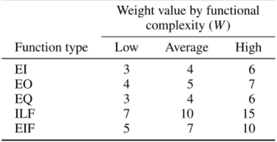
Table II. Unadjusted FP count calculation table. (Source:
IFPUG Counting Practice Manual 4.1, 1999.) Weight value by functional
complexity (W) Function type Low Average High
EI 3 4 6
EO 4 5 7
EQ 3 4 6
ILF 7 10 15
EIF 5 7 10
FP considering the maintenance environment, we need to introduce the new concept of the VAF. The VAFs of this model are related to the attributes of each characteristic group such as the engineer’s skill, technical characteristics and the maintenance environment. Finally, we suggest an exponential function model that can estimate how much effort is required for the software maintenance project.
3.2. Counting FPs
FPs of each application type should be counted to estimate the size of the maintenance project. There are three types of application maintenance such as adding, changing, and deleting. The rule of counting the function point is used as in the International Function Points User Group (IFPUG) model [9].
An application maintenance type could be one of the five function types: ILF, EIF, EI, EO, or EQ.
Each of these is individually assessed for complexity and given a weighting value that varies from three (for simple EIs) to 15 (for complex ILFs) as shown in TableII.
The unadjusted function count (FC) is computed by multiplying each raw count by the estimated weight (W):
FC=
function types
No. of functions×W (6)
where FC is the counted function point andWis the complexity weighting value of each function type.
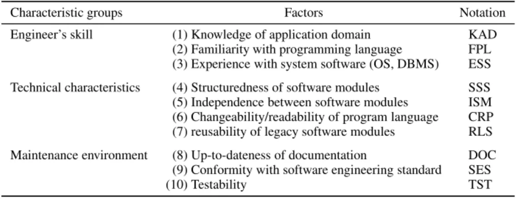
Table III. Value adjustment factors.
Characteristic groups Factors Notation
Engineer’s skill (1) Knowledge of application domain KAD (2) Familiarity with programming language FPL (3) Experience with system software (OS, DBMS) ESS Technical characteristics (4) Structuredness of software modules SSS (5) Independence between software modules ISM (6) Changeability/readability of program language CRP (7) reusability of legacy software modules RLS Maintenance environment (8) Up-to-dateness of documentation DOC
(9) Conformity with software engineering standard SES
(10) Testability TST
3.3. Adjusting the FPs 3.3.1. Value adjustment factors
This FC is then further modified by the 10 VAFs. In the SMPEEM model, the three types of VAFs are: (1) the engineer’s skill, considered as the perspective of ‘people’; (2) the technical characteristics considered as the perspective of ‘product’; (3) the maintenance environment characteristics considered as the perspective of ‘process’; as shown in TableIII.
The first characteristic group is the engineer’s skill required for the software maintenance, which includes three factors such as a knowledge of the application domain, familiarity with programming language, and experience with the system software (OS, DBMS). These factors describe the capability level of maintenance staff. If the application domain is well understood, the system requirements can be analyzed easily [2]. Also application experience, language and tool experience, and platform experience factors measure the productivity of COCOMO 2.0 [16].
The second technical characteristic group contains four factors, i.e. the structuredness of the software modules, the independence of the software modules, the changeability/readability of the programming language, and the reusability of the legacy software modules. These factors are representative of program modules status. As the software is maintained, its structure is degraded [2]. Application age [25] and reusability [16,26] factors are adopted as the technical productivity measures of software.
The last characteristic group is the maintenance environment which includes up-to-dateness of documentation, conformity with software engineering standards, and testability factors. These factors are more related to the maintenance process. Documentation matches with the lifecycle needs [16,26];
process maturity and testability [26] are referenced as the productivity factors to reduce maintenance costs.
These 10 factors are selected focusing on the perspective of maintenance project managers. In order to adjust the FP after counting it, as shown in Figure 1, some factors related to the size measures
of maintenance projects must be excluded; for example, maintenance traffic, size of software system or database. Because SMPEEM is aimed to estimate efforts in this phase, some factors related to output measures of estimation must also be excluded; for example the size of required efforts or team. Some factors related to maintenance organization characteristics for outsourcing can also be excluded because we consider only internal maintenance projects. We do not include the factors related to maintenance tools, because the responded organizations do not use any automatic maintenance tools.
3.3.2. Adjustment method
The unadjusted FP is multiplied by the VAF to produce the final FP. In SMPEEM, three characteristic groups of the 10 VAFs have a weighting value for each group and for each of the factors, respectively.
The VAF of a software maintenance project could be calculated from the following equation:
VAF= 3
group=1
k factors=1
scores×Wf 100
× Wg
100
(7) whereWgandWf are the weighting values of each characteristic group and their factors, respectively.
These weight values can be substituted from the value in TableIII. Scores are measured by the software maintenance project manager and vary from 0 (the lowest degree) to 5 (the highest degree), and are answered in part 2 of our questionnaire.
The VAF ranges from 0 to 50. This VAF can be used to adjust an unadjusted function count which was computed by Equation (6).
Alternatively, FPs can be computed by Equation (8), which is introduced for adjusting function counts as the unit of±δ%:
FP=FC×
1− δ
100
+ 2δ
5000
∗VAF (8)
whereδ is the absolute value of the adjustment range. The adjustment range can be decided by the actual data and repeated experiments of the concerned organization. For example, if an organization intends to adjust the function counts within the range of±20%,δof Equation (8) can be substituted with an absolute value of±20 to produce the following equation
FP=FC× {0.80+(0.008×VAF)} (9) From Equation (9), we obtain the adjusted FPs which can be used to calculate the estimated software maintenance effort. In the case of VAF=0, FP is calculated as 80% of the unadjusted function counts.
In contrast, the maximum VAF (50) provides 120% of the unadjusted function counts to final FPs.
Hence, Equation (8) gives us the adjusted FPs through the various adjustment ranges.
3.4. Estimation of software maintenance project effort
Software cost estimation models often have an exponential factor to account for the relative economies or diseconomies of scale encountered as a software project increases its size [16]. This factor is generally represented as the exponentBin the equation:
Effort=A×(Size)B
Table IV. Weight of characteristic groups (N=32).
Weight (Wg) 95% Confidence interval
t-test (df=31) of the difference Mean Standard
Characteristic groups (%) deviation T Significance Lower Upper
Engineer’s skill 36.7 9.6 0.011 0.991 −3.4263 3.4638
Technical characteristics 33.1 8.6 0.016 0.987 −3.0721 3.1221 Maintenance environment 30.2 9.9 0.025 0.980 −3.6048 3.5173
The relation between the software maintenance effort and FPs can be represented in the following exponential equation
Effort=a×FPb (10)
where the constantsaandbare the coefficients which can be introduced from the result of regression.
So, if FP and VAF of any maintenance project is known, the maintenance effort can be estimated by Equation (10).
4. VALIDATION
To validate the proposed SMPEEM empirically, a survey method was used. In this section, the summary of questionnaires and collected data will be described. For searching the best estimation model, regression analysis was performed by using the Statistical Package for the Social Science (SPSS), version 9.0.
4.1. Questionnaires
In this study, the questionnaire in the survey consists of two parts. The first part includes questions about the VAFs’ weight value covering the software maintenance project of most business applications.
The second part is for the collection of actual data about function points and maintenance efforts of past projects.
4.2. Data collection
To validate the proposed SMPEEM model, the actual data were collected from a survey of the system management (SM) organizations of four system integration (SI) companies in Korea.
For the sample of software maintenance project managers, a total of 44 questionnaires were distributed. 32 answers for part 1 and 26 answers of part 2 were collected.
Part 1 of our questionnaire asked to assign weights to the value adjustment factors listed in TablesIV and V. From these answers, we derive the mean and standard deviation. These average values are suitable as adjustment factors of SMPEEM if the variance is low.
Table V. Value adjustment factors of SMPEEM (N =32).
Weight (Wf) 95% Confidence interval
of the difference
Characteristic Mean Standard t Cronbach’s Factor’s
groups Factors (%) deviation (df=31) Significance Lower Upper alpha loading
Engineer’s KAD 45.0 13.7 0.000 1.000 −4.9316 4.9316 0.679 0.359
skill FPL 28.3 8.7 −0.012 0.990 −3.1448 3.1073 0.985
ESS 26.7 8.6 0.012 0.990 −3.0736 3.1111 0.924
Technical SSS 31.3 10.6 −0.027 0.979 −3.8809 3.7809 0.896 0.884
characteristics ISM 25.9 6.8 0.031 0.975 −2.4043 2.4793 0.836
CRP 21.9 11.2 −0.013 0.990 −4.0624 4.0124 0.912
RLS 20.8 5.3 −0.020 0.984 −1.9127 1.8752 0.862
Maintenance DOC 38.6 15.5 −0.002 0.998 −5.5811 5.5686 0.643 0.873
environment MET 29.1 11.8 −0.018 0.986 −4.2945 4.2195 0.758
TST 32.5 12.2 0.000 1.000 −4.3919 4.3919 0.646
In TableIV, the mean and standard deviation of the characteristic groups are shown. Each mean value was tested using the two-tailed one samplet-test at the 95% significance level. All significance probabilities (sig.) of TableIVare above significance level (0.05) and confidence intervals include zero.
For instance, significance probability (sig.) of characteristic group ‘engineer’s skill’ is 0.991> 0.05 and the confidence interval ranging from the lower (−3.4263) to the upper (3.4638) bound includes zero. The mean value (36.7) of this group can be supported. Likewise, these mean values of TableIV could be used as the weight value (Wg) in the SMPEEM model.
We also find that all significance probabilities (sig.) of TableVare above significance level (0.05) and confidence intervals include zero. For instance, the significance probability (sig.) of the ‘knowledge of application domain (KAD)’ is 1.000>0.05 and the confidence interval ranging from lower (−4.9316) to upper (4.9316) bound includes zero. Using the same approach, the mean values of 10 factors, shown in TableV, are calculated and can be used as the weight value (Wf) of adjustment factors after testing of the two-tailed one samplet-test.
For the collected data from part 1 of our questionnaire, reliability and validity tests were performed.
TableVshows the Cronbach’s alphas as they exceed 0.6. The factor’s loading values are the result of factor analysis using the extraction method of principle component analysis.
4.3. Regression analysis
Table VI shows the general descriptions of 26 maintenance projects collected from part 2 of the questionnaires.
For this dataset, we see the general description of these systems. These systems have an average of 169.1 source modules. The mean value of the age of the systems is 6.24 years. The programming language of the 22 systems is C, C++ or COBOL. The other four systems are written in PowerBuilder.
Table VI. General descriptions of projects (N=26).
Items Unit Mean value
System’s volume No. of source modules 169.1
Programming language Project 4 (Power Builder) 22 (C, C++ or COBOL)
System’s age Year 6.24
Size/project Function point 33.8
Maintenance effort/project Man-weeks 9.5
Table VII. Actual function point and efforts.
Project Unadjusted FP VAF Actual effort
1 31 3.27 5.7
2 18 3.56 3.6
3 28 3.58 5.7
4 18 3.15 1.4
5 18 3.04 1.4
6 21 3.25 2.8
7 11 2.84 2.1
8 46 2.89 5.0
9 28 1.80 6.1
10 23 2.84 2.8
11 27 2.46 4.0
12 22 3.41 5.3
13 68 3.37 20.5
14 57 3.01 12.9
15 23 3.15 3.1
16 19 2.65 2.8
17 26 2.68 4.6
18 53 1.90 13.4
19 140 4.05 50.2
20 28 3.25 3.0
21 13 2.66 2.7
22 16 3.77 1.7
23 44 3.54 15.0
24 23 3.28 4.0
25 60 2.41 12.9
26 17 2.79 2.0
Table VIII. Regression results by adjustment range.
Asymptotic 95% confidence interval
a b
Adjustment
range (%) a b R2 Lower Upper Lower Upper
±0 0.041 1.440 0.9654 0.0192 0.0626 1.3249 1.5554
±10 0.048 1.394 0.9660 0.0233 0.0717 1.2848 1.5033
±20 0.054 1.353 0.9664 0.0277 0.0811 1.2483 1.4572
±30 0.062 1.311 0.9648 0.0318 0.0924 1.2087 1.4140
±40 0.068 1.282 0.9639 0.0490 0.1006 1.1810 1.3834
±50 0.073 1.256 0.9613 0.0370 0.1090 1.1543 1.3585
±100 0.037 1.304 0.9647 0.1768 0.0570 1.2019 1.4058
±150 0.022 1.302 0.9646 0.0096 0.0348 1.2003 1.4043
±200 0.015 1.304 0.9649 0.0061 0.0241 1.2023 1.4060
Also, the average function points per maintenance project are 33.8 with a minimum of 11 and a maximum of 140. The average effort of maintenance project is 9.5 man-weeks, which is much smaller than the size of new development projects.
From part 2 of the questionnaire, unadjusted FPs of TableVII were estimated using the IFPUG model. VAFs were calculated according to the SMPEEM model. The responded projects include the add and change types of projects. Actual efforts were collected from the survey results and measured in man-weeks.
To evaluate the SMPEEM model, regression analysis is performed. Equation (10) was used for nonlinear regression analysis which describes the relation of actual efforts and adjusted FPs. The actual effort (man-weeks) and the FP values of TableVIIwere used in Equation (10) for each project.
The constantsa, bare the coefficients which resulted from the regression.
TableVIIIshows a summary of the regression analysis results. We sought the best regression model by varying the adjustment range from±0% to±200%. Regression coefficients (R2) of most models are above 0.9. Constantsaandbare significant in the asymptotic 95% confidence interval.
We obtain the highestR2valueR2=0.9664,F =259.90 in the model of adjustment range±20%.
This figure is meaningful considering the significant F value F0.95(3,25) = 2.99. In conclusion, Equation (10) can be rewritten as follows
Effort(man-weeks)=0.054×FP1.353 (11)
5. SUMMARY AND CONCLUSIONS
The SMPEEM is designed to help the project manager in charge of software maintenance to calculate the estimated software maintenance effort. Software maintenance means repairing defects in order to correct errors and adding small new features to software applications. In this model, the method of counting the FP to estimate the size of the maintenance is referred to as the FP model of the IFPUG.
Ten new VAFs are used for adjusting the FPs considering the software maintenance complexity characteristics. These VAFs are grouped into three categories, i.e. the engineer’s skill (people domain),
its technical characteristics (product domain) and the maintenance environment (process domain). Each weight of VAFs and the three characteristic groups is given by the mean value of collected data and validated by the t-test. The ten factors of the SMPEEM are simpler and adequate for assessing the maintenance effort.
With experimental analysis of the ranges of adjustment, the most significant regression model could be selected. We found that unadjusted FPs are a good measure to estimate the effort of the maintenance project and that they can be adjusted in the range of±20% by the 10 VAFs of SMPEEM. However, the 10 VAFs are not as influential as one expected.
We are aware that the collected data are only from small maintenance projects. Due to the limitations of the actual data, our SMPEEM should be refined by collecting and analyzing more actual projects if this model is to be applied to an organization. The result is that the methodology of SMPEEM may be used as a useful guide for the estimation of a maintenance project in any organization.
This study also can be further extended by using the maintenance projects of larger size software systems. These and similar investigations will provide a better estimation of the maintenance efforts based on productivity factors.
REFERENCES
1. Harrison W, Cook C. Insights on improving the maintenance process through software measurement. Proceedings International Conference on Software Maintenance. IEEE Computer Society Press: San Diego CA, 1990; 37–45.
http://www.cs.pdx.edu/∼warren/Papers/CSM.htm.
2. Sommerville I.Software Engineering. Addison-Wesley: Harlow, UK, 1996; 666–672.
3. Desharnais J, Pare F, Maya M, St-Pierre D. Implementing a measurement program in software maintenance: An experience report based on Basili’s approach.Proceedings of the Conference of the International Function Points Users Group.
International Function Points Users Group: Mequon WI, 1997; 143–152.
4. Martin J, Mcclure C.Software Maintenance: The Problem and its Solutions. Prentice-Hall: Englewood Cliffs NJ, 1983;
23.
5. Pigoski TM.Practical Software Maintenance: Best Practices for Managing Your Software Investment. Wiley: New York NY, 1997; 32–33.
6. Low GC, Jeffery DR. Function points in the estimation and evaluation of the software process.IEEE Transactions on Software Engineering1990;16(1):64–71.
7. Jones TC. Measuring programming quality and productivity.IBM System Journal1978;17(1):39–63.
8. Park R. Software size measurement: A framework for counting source statements.Report CMU/SEI-92-TR-20, Software Engineering Institute, Carnegie Mellon University: Pittsburgh PA, 1992.
9. IFPUG. Enhancement project function point calculation. Function Point Counting Practices Manual (Release 4.1).
International Function Points Users Group: Mequon WI, 1999; 8.10–8.17.
10. Kauffman R, Kumar R. Modeling estimation expertise in object based ICASE environments. Stern School of Business Report, New York University, 1993.
11. Banker R, Kauffman R, Kumar R. An empirical test of object based output measurement metrics in a CASE environment.
Journal of MIS1994;8(3):127–150.
12. Pressman RS.Software Engineering A Practitioner’s Approach, ch. 20. McGraw-Hill: New York NY, 1992; 677.
13. Boehm BW.Software Engineering Economics. Prentice-Hall: Englewood Cliffs NJ, 1981; 596–599.
14. Schaefer H. Metrics for optimal maintenance management. Proceedings Conference on Software Maintenance. IEEE Computer Society Press: Washington, 1985; 114–119.
15. Ministry of Information and Communication. Cost Estimation Guide for Software Business. Korean Ministry of Information and Communication: Seoul, Korea, 2002; 49–56.
16. Boehm BW, Clark B, Horowitz E, Westland C, Madachy R, Selby R. Cost models for future software life cycle process:
COCOMO 2.0.Annals of Software Engineering Special Volume on Software Process and Product Measurement, Arthur JD, Henry SM (eds.). Science Publishers: Amsterdam, 1995; 57–94.
17. Albrecht AJ. Measuring application development productivity. Proceedings of the joint SHARE/GUIDE and IBM Application Development Symposium. SHARE, Inc. and GUIDE Intl. Corp.: Chicagho IL, 1979; 83–92.
18. Albrecht AJ.AD/M Productivity Measurement and Estimate Validation. IBM Corporation: New York, 1984.
19. Desharnais J, Morris P. Validation of function points—an experimental perspective.Proceedings of the Conference of the International Function Points Users Group, Atlanta. International Function Points Users Group: Mequon WI, 1996;
167–184.
20. Symons CR. Function point analysis: Difficulties and improvement.IEEE Transactions on Software Engineering1988;
14(1):2–11.
21. Jones C. Applied software measurement.Assuring Productivity and Quality(2nd edn). McGraw-Hill: New York NY, 1997;
51.
22. SPR.User Guide to SPQR/20. Software Productivity Research Inc.: Burlington MA, 1987; 65.
23. Oman P, Hagemeister J, Ash D. A definition and taxonomy for software maintainability.Technical Report 91-08, Software Engineering Test Laboratory, University of Idaho, 1991.
24. Belady L, Lehman M. An Introduction to Growth Dynamics in Statistical Computer Performance Evaluation, Freiberger W (ed.). Academic Press: New York NY, 1972; 503–511.
25. Jorgensen M. Experience with the accuracy of software maintenance task effort prediction models.IEEE Transactions on Software Engineering1995;21(8):674–681.
26. Dart S, Christie AM, Brown AW. A case study in software maintenance.Report CMU/SEI-93-TR-8, Software Engineering Institute, Carnegie Mellon University: Pittsburgh PA, 1993.
AUTHORS’ BIOGRAPHIES
Dr Yunsik Ahn is a professor in the Department of Secretariat Science, Kyungwon College. He holds a BS from Jeonbuk National University, a ME in Computer Science from Yonsei University and a PhD in Information Management from Kookmin University.
Dr Ahn has more than 15 years of industry experience in information system projects and information technology consultancy. His current research interest lies in information system audit and software measurement.
Dr Jungseok Suh is a professor in the Department of Information Science, Korea Nazarene University. He has a doctorate degree from the Department of MIS at Kookmin University in Seoul Korea. He also has a Master of Science degree from Boston University, and a MBA degree, majored in MIS, from Drexel University. His current interest is in estimating for the developing component software.
Dr Seungryeol Kim is a professor in the School of MIS, Kookmin University Seoul Korea. He graduated from the Seoul National University and obtained a doctorate degree from the Department of IE at Iowa State University. He has been a lecturer in the Department of IE&M at California Polytechnic State University. His current research interest lies in two areas, object-oriented system analysis and design, and system measurement. He is also a member of the IFPUG.
Dr Hyunsoo Kimis a professor of MIS at Kookmin University in Korea. He holds a BE from Seoul National University, a MS from the Korea Advanced Institute of Science and Technology, and a PhD in Business Administration from the University of Florida.
His papers appear in Omega, European Journal of Operational Research, Intelligent Systems in Accounting, Finance and Management, MIS Research, etc. His research interest include information systems project management, cost estimation models, and information systems auditing.