Parameterizing anisotropic reflectance of snow surfaces from airborne digital camera observations in Antarctica

(1)

https://doi.org/10.5194/tc-14-3959-2020

Parameterizing anisotropic reflectance of snow surfaces from airborne digital camera observations in Antarctica

Tim Carlsen^1,a, Gerit Birnbaum², André Ehrlich¹, Veit Helm², Evelyn Jäkel¹, Michael Schäfer¹, and Manfred Wendisch¹

1Leipzig Institute for Meteorology, University of Leipzig, Leipzig, Germany

2Alfred Wegener Institute, Helmholtz Centre for Polar and Marine Research, Bremerhaven, Germany

anow at: Department of Geosciences, University of Oslo, Oslo, Norway Correspondence:Tim Carlsen (tim.carlsen@geo.uio.no)

Received: 6 April 2020 – Discussion started: 26 May 2020

Revised: 10 September 2020 – Accepted: 4 October 2020 – Published: 12 November 2020

Abstract.The surface reflection of solar radiation comprises an important boundary condition for solar radiative transfer simulations. In polar regions above snow surfaces, the surface reflection is particularly anisotropic due to low Sun elevations and the highly anisotropic scattering phase function of the snow crystals. The characterization of this surface reflection anisotropy is essential for satellite remote sensing over both the Arctic and Antarctica. To quantify the angular snow reflection properties, the hemispherical-directional reflectance factor (HDRF) of snow surfaces was derived from airborne measurements in Antarctica during austral summer in 2013/14. For this purpose, a digital 180^◦ fish- eye camera (green channel, 490–585 nm wavelength band) was used. The HDRF was measured for different surface roughness conditions, optical-equivalent snow grain sizes, and solar zenith angles. The airborne observations covered an area of around 1000 km×1000 km in the vicin- ity of Kohnen Station (75^◦0⁰S, 0^◦4⁰E) at the outer part of the East Antarctic Plateau. The observations include regions with higher (coastal areas) and lower (inner Antarc- tica) precipitation amounts and frequencies. The digital camera provided upward, angular-dependent radiance measurements from the lower hemisphere. The comparison of the measured HDRF derived for smooth and rough snow surfaces (sastrugi) showed significant differences, which are superimposed on the diurnal cycle. By inverting a semi- empirical kernel-driven bidirectional reflectance distribution function (BRDF) model, the measured HDRF of snow surfaces was parameterized as a function of solar zenith angle, surface roughness, and optical-equivalent snow grain size.

This allows a direct comparison of the HDRF measurements with the BRDF derived from the Moderate Resolution Imag- ing Spectroradiometer (MODIS) satellite product MCD43.

For the analyzed cases, MODIS observations (545–565 nm wavelength band) generally underestimated the anisotropy of the surface reflection. The largest deviations were found for the volumetric model weightfvol (average underestimation by a factor of 10). These deviations are likely linked to short- term changes in snow properties.

1 Introduction

Surface reflection in the polar regions plays an important role in the Earth’s climate system. The snow surface albedo is highly variable on both a temporal and spatial scale. This causes uncertainties in determining the surface solar radiative energy budget in these areas (e.g., Kuipers Munneke et al., 2008). As such it is essential to monitor the reflective properties of snow surfaces to accurately predict future climate change in the polar regions. However, their remote and harsh environment makes them difficult to access and requires remote sensing techniques to observe snow surface reflection and its influencing parameters.

The high spatial and temporal variability of the snow surface albedo necessitates continuous observations with global coverage, which are provided by satellite instruments. Polar- orbiting satellites monitor the reflectance (i.e., reflected radiance in units of W m⁻²sr⁻¹) at the top of the atmosphere (TOA). However, they are restricted in terms of the number

(2)

of available observation angles and spectral bands as well as their temporal resolution. The processing of using measurements from polar-orbiting satellites to monitor the broadband surface albedo typically requires three steps (e.g., Qu et al., 2015): atmospheric correction, modeling of the angular reflectance, and narrow-to-broadband conversion. During the first step, the TOA reflectance is converted into a surface reflectance by correcting for gaseous and aerosol scattering and absorption applying radiative transfer modeling (e.g., Vermote and Kotchenova, 2008). For the calculation of the narrowband surface albedo, accurate knowledge of the bidirectional reflectance distribution function (BRDF) of the surface is required due to the limited number of available observation angles. The BRDF describes the scattering of electromagnetic (EM) radiation from one incident direction to another direction of the hemisphere. By using a linear combination of the discrete spectral band measurements with specific weighting, the broadband surface albedo is calculated (e.g., Brest and Goward, 1987; Klein and Stroeve, 2002; Liang et al., 2003; Pohl et al., 2020). The largest uncertainty in this three-step process is introduced by the angular dependence of the surface BRDF, especially when the reflection of the underlying surface is highly anisotropic. This is the case for the reflection of solar radiation at snow surfaces in polar regions due to low Sun elevations and the anisotropic scattering phase function of snow crystals. As the snow surface of the Antarctic ice sheet is also used for the validation and cross-calibration of polar-orbiting satellites (Jaross and Warner, 2008), a thorough understanding of the anisotropic reflection is needed.

However, as an infinitesimal quantity, the BRDF of a surface cannot directly be measured under natural illumination conditions. From a rigorous physical point of view, most satellite, airborne, and ground-based instruments measure the hemispherical-directional reflectance factor (HDRF;

Schaepman-Strub et al., 2006) if the reflectance is constant over the full cone angle of the instrument’s field of view (FOV). In contrast to the BRDF, the HDRF includes incident irradiance from the entire hemisphere. An effective BRDF can only be derived from HDRF observations if the atmospheric influence is considered and the FOV is sufficiently small (e.g., Gatebe et al., 2003; Lyapustin et al., 2010).

For example, the retrieval of the aerosol optical depth (AOD) over highly reflecting surfaces is complicated, as it is hard to separate the surface and aerosol contributions to the measured reflectance at the TOA (Tomasi et al., 2015), especially for the comparably low values of AOD in polar regions (Mei et al., 2013). Due to its high surface albedo, most of the solar radiation incident on a snow surface is reflected, which depends strongly on the BRDF of the snow surface and, thus, on the illumination and viewing geometry. In general, most of the photons are scattered by the snow grains in the forward scattering direction. Yang et al. (2014) compared Moderate Resolution Imaging Spectroradiometer (MODIS) measurements of AOD at 550 nm over eastern China with ground-

based data from the Aerosol Robotic Network (AERONET).

Using a Lambertian model, 54 % of the regression points fell within the expected error envelope around the 1:1 line.

This result is improved to 69 % if a more sophisticated, non- Lambertian model accounting for anisotropic reflection at the land surface is applied.

Yet the BRDF varies with snow grain morphology, the solar zenith and azimuth angles, the liquid water content of the snowpack, the snow impurity type and concentration, the dimension and orientation of surface roughness structures, and the wavelength. To account for these effects, an accurate model of the snow BRDF is needed. A BRDF model can be physical, empirical, or semi-empirical. Physical BRDF models (e.g., Cook and Torrance, 1982) accurately simulate the scattering of an EM wave at a surface by applying physical laws. The high accuracy comes at the cost of very complex computations. Empirical BRDF models (e.g., Phong, 1975;

Walthall et al., 1985) mimic the surface reflection by means of a simple, non-physical formulation. However, the draw- back of the rather simple computations is their restricted accuracy. Semi-empirical models (e.g., Martonchik et al., 1998;

Lucht et al., 2000) use simple, direct parameterizations of a more complex physical BRDF with a limited number of independent parameters.

The anisotropic reflection by snow surfaces was investigated by Li (1982) with simulations of the snow BRDF using Mie theory and the doubling and adding method. Apply- ing Mie theory and the discrete-ordinate method, Han (1996) retrieved the surface albedo from satellite measurements in the Arctic. Leroux and Fily (1998) developed a snow BRDF model including the effect of sastrugi by means of regu- larly spaced, identical, and rectangular protrusions. Leroux et al. (1998) and Leroux et al. (1999) employed the doubling and adding method, Mie theory, and ray tracing to develop a snow BRDF model including polarization. Comparing the simulated values with observations in the principal plane, they found that the BRDF in the near-infrared wavelength range is strongly affected by the snow grain shape, whereby simulations assuming hexagonal particle shapes yield an improved agreement with the observations compared to assuming spheres. Accordingly, Aoki et al. (2000) stressed the importance of the particle shape assumption for the scattering phase function used in their BRDF model (applying both Mie theory and the Henyey–Greenstein phase function) when comparing to observations between 0.52 and 2.21 µm wavelength. Kokhanovsky and Zege (2004) demonstrated the use of an asymptotic analytical equation to model the BRDF of snow. Their approach represents the snow grains for example as fractal particles and, thus, accounts for their non-sphericity. Evaluating this asymptotic model with in situ measurements of the snow reflectance, Kokhanovsky et al.

(2005) found generally good agreement but reduced model accuracy in the solar principal plane at large observation angles. In contrast to considering snow grains as independent scatterers of fractal shape, Malinka (2014) provided a frame-

(3)

work to calculate the inherent optical properties (extinction coefficient, single-scattering albedo, scattering phase function, and the polarization properties) by applying the concept of stereology, which considers snow as a random mixture of ice and air. Malinka et al. (2016) combined the stereological approach with analytical, asymptotic formulas to calculate the bidirectional reflectance. Their model showed high accuracy when compared to albedo observations of snow-covered sea ice.

The comparison of in situ measurements of the snow reflectance with simulations is essential in terms of model validation. Observations of the HDRF (or effective BRDF in case the FOV is small and the atmospheric influence is considered) are conducted using a variety of different measurement concepts. For ground-based applications, manual or automated gonio-spectrometer systems are employed (e.g., Painter et al., 2003; Pegrum et al., 2006; Bourgeois et al., 2006a). Kuhn (1985) observed a peak in reflectance that is contained within±60^◦to both sides of the solar azimuth angle. This peak becomes more prominent with increasing solar zenith angle and snow grain size. Marks et al. (2015) measured the HDRF of snow surfaces between 400 and 1600 nm wavelength with the Gonio Radiometric Spectrometer Sys- tem (GRASS; Pegrum et al., 2006) at Dome C, Antarctica.

Their observations also showed enhanced forward scattering. In addition, they observed a larger anisotropy of the surface reflection at longer wavelengths. Employing a gonio- spectrometer, Bourgeois et al. (2006b) measured strong variations of the HDRF between 0.6 and 13 (in the wavelength range 350–1050 nm) depending on the solar zenith angle and the surface roughness at Summit, Greenland. Mea- surements with the Automated Spectro-Goniometer (ASG;

Painter et al., 2003) showed a decrease of snow HDRF at all wavelengths between 400 to 2500 nm when the snow grain size increased from 80 to 280 µm (Painter and Dozier, 2004b). Further comparisons with the results of a forward discrete-ordinate radiative transfer model (Stamnes et al., 1988) revealed larger deviations between the simulations and observations for more complex crystals. The importance of the crystal habit for the anisotropy of reflection at snow surfaces was also emphasized by Dumont et al. (2010) and Stan- ton et al. (2016). The latter measured increasing anisotropy of the surface reflection during the growth of surface hoar in the laboratory. Several studies observed systematically less anisotropy for a typical snow HDRF than estimated from simulations (Warren et al., 1998; Painter and Dozier, 2004a;

Hudson et al., 2006; Hudson and Warren, 2007). In the solar principal plane, the models mainly overestimate the forward scattering and underestimate the backward scattering. Im- plementing non-spherical grains in the BRDF models (e.g., Mishchenko et al., 1999; Xie et al., 2006; Jin et al., 2008) im- proves the comparison with observations. The non-spherical model of Jin et al. (2008) agrees within±10 % for viewing zenith angles less than 60^◦ with observations in Antarctica performed by Hudson et al. (2006). However, the asymme-

try between forward and backward scattering still remains.

This highlights the need to further incorporate macroscopic effects such as the roughness of the snow surfaces into the models (Leroux and Fily, 1998; Hudson and Warren, 2007).

Ground-based instruments observe the directional reflectance of a characteristic, homogeneous surface, whereas airborne and satellite observations average over a larger measurement area. Thus, the latter are more suitable for studying the influence of macroscopic surface roughness on the surface HDRF. Nolin et al. (2002) employed multi-angular measurements with the Multi-angle Imaging Spectroradiometer (MISR) for the characterization of surface roughness over Greenland and Antarctica. Measurements with the Clouds and the Earth’s Radiant Energy System (CERES) showed monthly regional biases between−12 and 7.5 W m⁻²in the cloudless TOA solar irradiance. These biases were attributed to the effect of sastrugi, which introduce a significant solar azimuth dependence: Kuchiki et al. (2011) observed a diurnal cycle in MODIS reflectances over the South Pole. In general, sastrugi decrease the forward scattering by casting shadows and increase the backward scattering due to a lower effective incident angle caused by the sastrugi slope, and the snow HDRF loses its azimuthal symmetry (Warren et al., 1998).

Zhuravleva and Kokhanovsky (2011) simulated a larger effect for a higher density of the sastrugi field.

Airborne measurements can be employed for the validation of BRDF models and the comparison with the large pixel size of satellite observations. Gatebe and King (2016) provided an extensive database of airborne spectral (effective) BRDFs for various surface types, for example, ocean, vegetation, snow, desert, and clouds. The effective BRDFs were acquired by the Cloud Absorption Radiometer (CAR;

Gatebe et al., 2003) over a 30-year period between 1984 and 2014. The CAR is a scanning radiometer covering 14 spectral channels between 340 and 2324 nm. The effect of surface roughness on the effective BRDF was studied by Lyapustin et al. (2010) with CAR measurements during the Arctic Re- search of the Composition of the Troposphere from Aircraft and Satellites (ARCTAS) spring campaign in April 2008 (Ja- cob et al., 2010; Matsui et al., 2011). Their results showed an agreement between the kernel-based Ross-Thick–Li-Sparse- Reciprocal (RTLSR) BRDF model (Lucht et al., 2000) used in the operational MODIS BRDF/Albedo Model Parameters product (MCD43A1) (Schaaf et al., 2002) and the CAR measurements to within ±0.05. The RTLSR model performed better in the forward scattering direction, whereas the kernel- based Modified Rahman–Pinty–Verstraete (MRPV) BRDF model (Martonchik et al., 1998) used for the processing of data from MISR performed better in the backscattering direction. Jiao et al. (2019) proposed an additional snow kernel within the kernel-driven BRDF model framework to better account for the anisotropic reflection of pure snow surfaces. Incorporating the additional snow kernel yielded a correlation coefficient of 0.9 (compared to 0.65 for the original three-kernel model) and only small biases between the model

(4)

and different BRDF validation data from ground-based and satellite observations.

Cox and Munk (1954) analyzed radiance-calibrated ana- log photographs for the parameterization of the ocean HDRF.

Nowadays, digital cameras are increasingly applied in vegetation and soil monitoring (e.g., Lebourgeois et al., 2008;

Koukal and Atzberger, 2012). The instantaneous measurement of multiple viewing angles facilitates aerial HDRF measurements with digital cameras. The high angular resolution allows the detection of features in the anisotropy of the reflection which could be missed with HDRF measurements allowing only a limited number of observation angles.

This was demonstrated by Goyens et al. (2018) for ground- based measurements of the snow HDRF, comparing radiance measurements with a spectroradiometer at discrete viewing angles with hyperangular observations using a fish-eye radiance camera. Ehrlich et al. (2012) used a commercial digital camera equipped with a wide-angle lens with a FOV of 100^◦ for measurements of the HDRF of snow-covered sea ice, ocean, and clouds (viewing zenith angle up to around 60^◦).

This study presents a method to derive the snow HDRF at a visible wavelength (spectral band 490–585 nm) from airborne digital camera measurements in Antarctica during austral summer in 2013/14. Concurrent measurements of the optical-equivalent snow grain size retrieved from spectral surface albedo measurements, and surface roughness determined by means of a laser scanner, allow for investigating their effect on the snow HDRF in separate case studies. Sub- sequently, the measurements are used to parameterize the snow HDRF applying the RTLSR model (Lucht et al., 2000).

The presented methodological approach allows for a direct comparison of the airborne HDRF measurements with satellite observations from MODIS.

The definition of reflectance quantities used within this work, the modeling of the BRDF, and the inversion of a semi-empirical kernel-driven BRDF model are presented in Sect. 2. The fieldwork and instrumentation are presented in Sect. 3 together with the detailed calibration involved in the measurement of the snow HDRF. The dependence of the snow HDRF on the solar zenith angle, the surface roughness, and the optical-equivalent snow grain size is studied in Sect. 4 based on three cases. Subsequently, the airborne measurements are compared with satellite-derived BRDF from MODIS. In the concluding Sect. 5, the findings of this work are summarized and perspectives for future studies are given.

2 Methodology

2.1 Definition of reflectance quantities

The definition of the reflectance quantities applied within this work follows Schaepman-Strub et al. (2006). The intrinsic reflectance properties of a surface are given by its

BRDF. It quantifies the reflection of the incident radiation at the surface and its scattering from one direction of the hemisphere to another. The spectral BRDF (f_BRDF, units of sr⁻¹) provides for each zenith (θ_i) and azimuth angle (ϕ_i) of incident direct irradianceF_i(θ_i, ϕ_i;λ)the reflected radiance I_r(θ_i, ϕ_i;θ_r, ϕ_r;λ)for all directions of reflection (defined by the reflection zenith and azimuth anglesθ_randϕ_r) by f_BRDF=dIr(θi, ϕi;θr, ϕr;λ)

dFi(θi, ϕi;λ) . (1)

The bidirectional reflectance factor (BRF, dimensionless) is obtained when the BRDF of a sample surface is divided by the BRDF of a diffuse (Lambertian) standard surface illumi- nated under the same conditions (identical beam geometry).

As the BRDF of an ideal Lambertian surface is(πsr)⁻¹, the BRF is given by

R_BRF=dIr(θi, ϕi;θr, ϕr)

dFi(θi, ϕi) · dFi(θi, ϕi)

dI_r^ideal(θi, ϕi)=πsr·f_BRDF. (2) In Eq. (2) and in the remainder of this section, the spectral dependence is omitted for reasons of simplicity. In atmospheric conditions, both the BRDF and BRF cannot be measured directly as the global irradianceF0 reaching the surface is composed of a direct (F_i) and diffuse (F_diff) com- ponent. In this case, the measurable quantity is the HDRF.

The definition of the HDRF is analogous to that of the BRF but includes irradiance from the entire hemisphere (denoted with 2π):

RHDRF=πsr·dI_r(θ_i, ϕ_i,2π;θ_r, ϕ_r) dF₀(θ_i, ϕ_i,2π )

=R_BRF(θ_i, ϕ_i;θ_r, ϕ_r)·f_dir

+R(2π;θ_r, ϕ_r)·(1−f_dir) . (3) fdir denotes the fraction of direct incident radiation (i.e., fdir∈ [0,1]). The second step in Eq. (3) assumes that the incident diffuse radiation is isotropic (for details, see Schaepman-Strub et al., 2006). The additional integration over all reflection angles leads to the bihemispherical reflectance, generally called surface albedoα.

2.2 Modeling of the bidirectional reflectance

The shape of the BRDF is described by a weighted sum of trigonometric functions, generally referred to as kernels for volumetric scattering (K_vol), geometric scattering (K_geo), and isotropic scattering (K_iso).

The kernel-driven semi-empirical Ross–Li model (Lucht et al., 2000), which forms the basis of the MODIS 16 d BRDF/albedo product (Schaaf et al., 2002), is applied within this study. The BRDF is given as a linear combination of the kernels with corresponding non-negative weighting func-

(5)

tionsfiso,fvol, andfgeo:

f_BRDF(θi, θ_r, 1ϕ, λ)=f_iso(λ)·K_iso

+f_vol(λ)·K_vol(θ_i, θ_r, 1ϕ)

+fgeo(λ)·Kgeo(θi, θr, 1ϕ) , (4) with the viewing (reflection) zenith angleθr, incidence zenith angleθ_i, relative viewing azimuth angle1ϕ, and wavelength λ. The kernels,

K_iso=1, (5)

Kvol=

π 2−θ

cosθ+sinθ cosθ_i+cosθ_r −π

4, (6)

K_geo=O(θ_i, θ_r, 1ϕ)−secθ_i−secθ_r +1

2(1+cosθ )·secθ_i·secθ_r, (7) depend on the scattering angleθand the functionO:

cosθ=cosθ_i·cosθ_r+sinθ_i·sinθ_r·cos1ϕ, (8) O(θ_i, θ_r, 1ϕ)= 1

π(C−sinC·cosC)·(secθ_i+secθ_r) . (9) The functions C andD depend solely on the viewing and illumination geometry:

cosC= 2·

q

D²+(tanθ_r·tanθ_i·sin1ϕ)²

secθ_i+secθ_r , (10)

D= q

tan²θr+tan²θi−2 tanθr·tanθi·cos1ϕ. (11) Originally, the concept of the model was developed studying typical features in observations of the bidirectional reflectance of various surface types (Roujean et al., 1992).

First, bare soil surfaces exhibit strong backscattering characteristics and show the effect of geometrical structures on the surface. Secondly, dense leaf canopies typically feature a minimum reflectance close to the nadir direction that increases off nadir for all azimuthal directions. In their approach, Roujean et al. (1992) represented the modeled BRDF as a linear combination of these two observational characteristics – with the former being accounted for byKgeo, and the latter byKvol. The volumetric kernelKvolstems from volume scattering radiative transfer models (Ross, 1981). Thereby, randomly located facets that absorb and scatter incident radiation are modeled under the single-scattering approximation. The formula given in Eq. (6) corresponds to the Ross- Thick kernel for a dense leaf canopy. The geometric kernel K_geo is derived from surface scattering and geometric shadow casting theory (Li and Strahler, 1992) and expresses effects caused by intercrown gaps within vegetation. It represents randomly oriented vertical protrusions on a flat and horizontal surface that isotropically reflect radiation. Equa- tion (7) gives the Li-Sparse geometric kernel in reciprocal

form describing the casting of shadows by a sparse ensemble of surface objects.

Hu et al. (1997) validated kernel-based BRDF models with 27 multi-angular data sets from various land cover types. The accuracy of the model was high. The correlation coefficient between model and observations was above 0.7 for all and above 0.9 for more than half of the data sets. Although originally calculated for surfaces covered with vegetation, the Ross-Thick and Li-Sparse-Reciprocal kernels are also applied for snow surfaces for the MODIS BRDF/albedo product. Stroeve et al. (2005) and Stroeve et al. (2013) assessed the accuracy of the 16 d albedo product of 11 years of measurements at 17 automatic weather stations on the Greenland ice sheet. They retrieved physically realistic ice sheet albedo values with an overall mean bias between MODIS and the in situ measurements of 0.022.

2.3 Inversion of semi-empirical kernel-driven model The main benefit of retrieving the weighting functionsfiso, fvol, and fgeo from the HDRF measurements is that they encompass all of the angular radiance information. The retrieval is done by inverting the RTLSR BRDF model. Thus, information about the complete two-dimensional shape of the HDRF is used.

The modeled f_BRDF(θi, θ_r, 1ϕ, λ) from Eq. (4) can be written in the form of a sum as

f_BRDF,l=

3

X

k=1

f_k·K_kl. (12)

The spectral dependence is omitted here, and the index l denotes a particular viewing and illumination geometry (θi, θr, 1ϕ)_l. Considering an observation withN directional measurementsρl (l=1, . . ., N), the error functionE²is defined as the difference between the observed and the modeled reflectances such that

E²=1 d

N

X

l=1

ρl−fBRDF,l2

wl

. (13)

The degree of freedomd is(N−3)andw_l denotes weights which are assigned to the respective observations. In general, wl could take the values 1,ρl, orρ_l². The goal of the inversion is the determination of the model weighting functionsfk

such thatE² is minimized. Strahler et al. (1996), amongst others, presented the analytical solutions for the threefk fol- lowing this minimization. and Lewis (1995) showed thatE² has a global minimum inf_k.

The inversion depends on the choice of the error function E² and, thus, on the choice of the weightsw_l. Minimizing the absolute error (using weights equal to unity) leads to smaller errors in angular domains with a large reflectance.

In contrast, minimizing the relative error (e.g.,w_l=ρ_l, ρ_l²) performs better in angular regions with lower reflectance.

(6)

Subsequently, different choices forwlwere tested for the retrievals performed in this work, andwl=ρ_l²was chosen as it produced the lowest retrieval errors across the entire angular domain.

3 Measurements and instrumentation

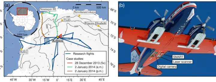
The airborne measurements were performed with the Polar 6 research aircraft (Wesche et al., 2016), operated by the Alfred Wegener Institute, Helmholtz Centre for Polar and Marine Research (AWI), Bremerhaven, Germany. Polar 6 was based at Kohnen Station (75^◦0⁰S, 0^◦4⁰E). Figure 1a illustrates the tracks of the research flights with Polar 6 (60 flight hours) covering an area of 1000 km×1000 km around Kohnen Sta- tion in Dronning Maud Land. The flights were performed between 24 December 2013 and 5 January 2014. The observations comprised regions with higher (coastal areas) and lower precipitation amounts and frequencies (inner Antarc- tica), as well as a variety of surface roughness structures. An overview of the airborne instrumentation is given in Carlsen et al. (2017); the mounting of the digital camera, laser scanner, and the Spectral Modular Airborne Radiation measurement sysTem (SMART) for surface albedo measurements on the underside of the aircraft is illustrated in Fig. 1b. The variability of the solar zenith angle is illustrated in Fig. 2a in the form of a histogram. During the flights, the solar zenith angle varied between 49 and 73^◦.

3.1 Surface roughness measurements using a laser scanner

The snow surface topography was measured using the airborne laser scanner RIEGL VQ-580. In time-of-flight laser ranging, a near-infrared laser beam (1064 nm wavelength) is emitted downward and subsequently reflected upward by the snow surface before the echo is acquired by the sensor. From the time lag between emission and detection, the distance to the ground is calculated with a precision of about 25 mm depending on flight altitude. A fast-rotating polygonal mirror with a FOV of 60^◦and 10 to 150 scans per second allows for fully linear, unidirectional, and parallel scan lines.

After a correction for the aircraft attitude, a 1 km×1 km digital elevation model (DEM) is generated from the geo- tagged laser point cloud with a resolution of 1 m. Subtract- ing the large-scale topography (smoothed DEM), the residual field contains the roughness information. The standard deviation (SD) of the residual field is interpreted as the surface roughness at the central coordinate of the DEM. Thus, roughness data are given for one data point per 1 km along the flight track of the aircraft. The uncertainty of the absolute height measurements (used for DEM generation) is less than 0.1 m. The relative analysis applied to the measurements yields even higher accuracy.

The range in surface roughness is illustrated in Fig. 2b in the form of a histogram. The snow surface was generally smooth with roughness structures mostly below 5–10 cm (note the logarithmic scale; maximum: 2.2 m).

3.2 Optical-equivalent snow grain size as retrieved from spectral surface albedo measurements Solar spectral radiation measurements were conducted using SMART (Wendisch et al., 2001; Ehrlich et al., 2008). The upward and downward spectral irradiance [F^↑(λ), F^↓(λ)]

is measured within 0.3 to 2.2 µm wavelength applying an active horizontal adjustment system of the optical inlets to compensate for aircraft movement. From the irradiance measurements, the spectral snow surface albedo was obtained (Wendisch et al., 2004). The spectral resolution is 2 to 3 nm between 0.3 and 1.0 µm and 15 nm up to 2.2 µm wavelength;

the temporal resolution is in the order of 1 s. Combining the errors associated with the signal-to-noise ratio (1.3–3.0 %), the accuracy of the dark correction (0.1 %), the wavelength calibration (1.0 %), the accuracy of the cross-calibration (1.0–4.5 %), the non-ideal cosine response of the optical inlets (3.5 %), and the horizontal stabilization (1.0 %), the surface albedo measurements with SMART have an estimated uncertainty between 4.1 and 8.1 % depending on wavelength (Carlsen et al., 2017).

The optical-equivalent snow grain size is defined as the radiusRoptof a collection of spheres with the same volume- to-surface ratio compared to the actual non-spherical snow grains. The retrieval of Ropt from spectral surface albedo measurements is described in Carlsen et al. (2017). In principle, the snow grain size and pollution amount (SGSP) algorithm (Zege et al., 2011) was extended to spectral ra- tios of surface albedo at 1280 and 1100 nm wavelength.

Being independent of systematic measurement uncertainties (e.g., cross-calibration of the optical inlets), this approach decreases the uncertainty of the retrieved R_opt compared to the single-wavelength approach. The retrievedR_optfrom SMART and analogous ground-based measurements were compared to grain size observations utilizing reflectance measurements with MODIS (Carlsen et al., 2017). The grain size as retrieved from SMART measurements (mean value: 105 µm) is slightly higher than the MODIS retrievals (89 µm). The larger data set of ground-based observations (72 µm) agrees well with the MODIS retrievals within the ranges given by the measurement uncertainties (linear correlation coefficient: 0.78; root-mean-square error: 24 µm).

The variability ofRoptduring the research flights is illustrated in Fig. 2c in the form of a histogram. The optical- equivalent snow grain size varied between 16 and 480 µm but was mostly below 120 µm depending on precipitation and snow metamorphism processes.

(7)

Figure 1. (a)Illustration of research flights with Polar 6 in Dronning Maud Land between 24 December 2013 and 5 January 2014. The five flights on 28 December 2013 (marked in red) and the two flights on 2 January 2014 (green and brown) are used for the case studies. The parameter ranges covered by the case studies are marked with the same colors within the histograms in Fig. 2.(b)Photograph of Polar 6 illustrating the mounting of the digital camera, SMART, and the laser scanner.

Figure 2.Variability of different parameters during research flights shown as histograms of the probability density function (PDF). The parameter ranges covered by the case studies are marked with the same colors as the corresponding flight tracks in Fig. 1.(a)Vari- ability of solar zenith angle (bin size: 1^◦).(b)Variability of surface roughness (bin size: 4 cm). Note the logarithmic scale.(c)Variabil- ity of optical-equivalent snow grain size (bin size: 20 µm).

3.3 Directional radiance measurements using a digital camera

3.3.1 Camera specifications

A Canon EOS-1D Mark III digital camera was used for the airborne HDRF measurements of the snow surface. It is a

digital single-lens reflex camera with a complementary metal oxide semiconductor (CMOS) image sensor. The CMOS sensor covers 3908 pixel×2600 pixel on a sensor area of 28.1 mm×18.7 mm (Advanced Photo System (APS-H) format). During the observations, the camera was configured with a 8 mm F3.5 EX DG Circular Fisheye lens by Sigma.

Color information is obtained by means of a color filter ar- ray (CFA) in front of the CMOS sensor. The CFA consists of red (R), green (G), and blue (B) color filters, which determine the spectral response of the underlying pixel.

In principle, the measured signal s (in digital numbers, DN) should be saved essentially verbatim in the propri- etary RAW format CR2 (Canon RAW version 2). This would ensure the highest flexibility in the data analysis as no interpolation or white balance color correction is applied to the raw data. Full control over the post-processing steps is a prerequisite for radiometric measurements. Dur- ing the airborne measurements, the camera was set to pro- duce sRAW output format (small RAW) with a resolution of 1944 pixel×1296 pixel. At some point, internal chrominance subsampling is applied by the camera (Kerr, 2015).

The sRAW photos are decoded utilizing the open-source tooldcraw(Coffin, 2017). The darkness level was set to 0 DN (see below) and the saturation level to 16 383 DN as the camera captures images with color depth of 14 bit. In between, the raw data are linearly interpolated. The multipliers for all channels are set to 1, meaning no white balance color correction is applied. The dynamic range of the output file is 16 bit (saturation at 65 536 DN).

To characterize the linearity of the sensor, photos from the radiation emitted by an integrating sphere with varying output intensities were taken with the camera in the laboratory (Carlsen, 2018). The camera sensor showed a lin-

(8)

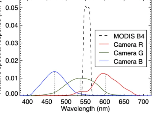
Figure 3.Relative spectral response functions for the three camera channels (colored lines: R, G, and B). The vertical dotted lines denote the respective central wavelengths. Dashed black line: RSR function for MODIS spectral band 4.

ear sensitivity over a large part of the dynamic range up to 53 000 DN; the coefficient of correlation was exceptionally high at 0.99998. Photographs that measured higher signals (0.4 % of the total number) were excluded from the analysis.

Compared to the dynamic range, the dark current (5 DN) and the read-out noise (7 DN) can be neglected.

Information on the spectral response of the camera is needed for the radiometric calibration. It determines the ex- tent to which radiation of a certain wavelength passes the fish-eye lens as well as the CFA and is registered by the pho- todiodes. In this regard, the relative spectral response (RSR) function (in units of nm⁻¹) of the three camera channels is defined as

RSR(λ)= Tc(λ)

∞

R

0

T_c(λ)dλ

. (14)

T_c(λ) withc=R, G, B denotes the dimensionless spectral transmission coefficients. The RSR function is normalized such that

∞

Z

0

RSR(λ)dλ=1. (15)

The RSR function of the camera was measured in the laboratory using an integrating sphere as a radiation source and varying the outgoing radiation between 300 and 750 nm in increments of 5 nm wavelength by means of a grating monochromator. Figure 3 shows the measured RSR functions for the three camera channels. The central wavelengths of the non-Gaussian RSR functions are 602 nm (R), 538 nm (G), and 470 nm (B). Their full width at half maximum (FWHM) varies between 68 nm for the blue channel and 95 nm for the green channel.

The FOV of the camera is 180^◦due to the optics of the fish- eye lens. However, the camera is installed slightly above the

lower aircraft body so that the camera is protected especially during take-off and landing. Therefore, parts of the aircraft frame are constantly in the FOV of the camera, which is why the effective FOV is reduced to approximately 160^◦. 3.3.2 Radiance calibration and image post-processing The post-processing of each raw image involves (a) the radiometric calibration, (b) the geometric calibration, (c) the aircraft attitude correction, and (d) the calculation of the HDRF.

A detailed description of the different steps can be found in Carlsen (2018).

The measured signal was converted into the physical quantity of radiance (units of W m⁻²nm⁻¹sr⁻¹) by means of a radiometric calibration in the laboratory. The pixels respond differently to a uniform illumination due to manufacturing tolerances (e.g., irregularities in the silicon used), contami- nation with dust particles, and optical effects at the edges of the lenses. These deviations lead to the photo response non- uniformity (PRNU) and need to be corrected.

The camera was positioned in front of an integrating sphere that served as a uniform radiation source. However, a distinct decrease in brightness is visible from the center to the edges of the sensor. This vignetting effect is typical for digital cameras (e.g., Lebourgeois et al., 2008). From the data sheet, the spectral radianceI_sphere(λ)that the integrating sphere emits at the specific optometer current is known. The calibration factorkcis defined at each pixel location on the sensor (rowx, columny) as

k_c(x, y)=Isphere(λ)

s(x, y) ·t_exp (16)

and carries the unit of W m⁻²nm⁻¹sr⁻¹(DN/s)⁻¹. During the calibration, the exposure timet_exp was set to 1/1000 s.

Not only doesk_c correct for the PRNU; it simultaneously performs the absolute calibration, transforming the measured digital signal into the physical quantity of radiance (in units of W m⁻²nm⁻¹sr⁻¹).

The geometric calibration of the camera–lens system re- lates each sensor pixel to a viewing zenith and azimuth angle (θ_v,ϕ_v). Often, the process of geometric calibration of a camera involves calibration equipment or the use of pla- nar targets such as checkerboard patterns (e.g., Tsai, 1987;

Urquhart et al., 2016). Within this work, a stellar calibration method is applied (e.g., Schmid, 1974; Klaus et al., 2004;

Mori et al., 2013; Urquhart et al., 2016) utilizing the high precision to which the positions of stellar objects are known.

In this regard, 684 different star positions identified in sub- sequent pictures of the night sky were utilized to calculateθ_v andϕ_vfor each sensor pixel.

(9)

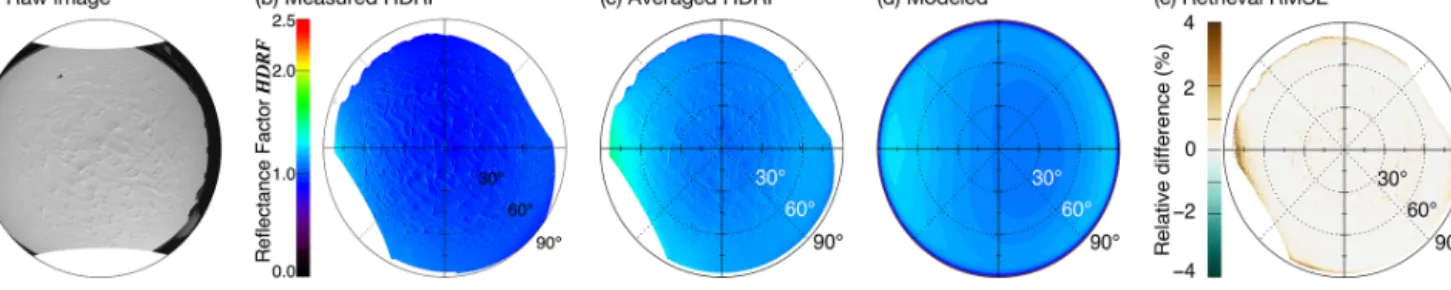
Figure 4.Exemplary post-processing and retrieval of model parameters for HDRF measurement.(a)Raw image taken on 2 January 2014 at 08:16 UTC (θ₀=58.9^◦).(b) Polar plot of observed snow HDRFρ_l calculated from raw image for camera channel G. The image is rotated in the azimuthal direction of the Sun such that the Sun is on the left.(c)Averaged HDRF measurement using three images; the footprint is 1670 m.(d)Modeled snow HDRFR_HDRF,lafter retrieval of model parametersf_iso=1.12,f_vol=0.17, andfgeo=0.01 from(c).

(e) Relative difference(ρ_l−R_HDRF,l)/R_HDRF,l. The accumulated RMSE is 0.04.

3.4 Calculation and uncertainties of measured surface HDRF

The camera took pictures with a temporal resolution of about 8 s. Exemplarily, Fig. 4 demonstrates the derivation of the snow HDRF from a raw image taken by the camera on 2 Jan- uary 2014 (08:16 UTC; see Fig. 4a). First, the pixels receiv- ing radiation from the direction of the aircraft frame are excluded. For each pixel location (x,y), the radianceI (x, y) (in units of W m⁻²nm⁻¹sr⁻¹) is calculated from the measured signalsusing the absolute calibration factork_cand the exposure timetexp:

I (x, y)=s(x, y)

t_exp ·k_c(x, y). (17)

The camera viewing angles are calculated from the geometric calibration for each pixel (x,y). As the camera is fixed to the aircraft frame, a correction for the aircraft attitude was implemented to obtain the reflection anglesθrandϕr. Thus, beside the geometric calibration, the observed reflection angles are determined by the attitude angles of the aircraft. Uti- lizing the data from the internal navigation system and the GPS on Polar 6, the viewing angles are corrected depending on the roll, pitch and yaw angles of the aircraft at the time of measurement. In this regard, Euler rotations are applied as described in Ehrlich et al. (2012). Finally, the observed HDRF is calculated by

R_HDRF(θ₀, ϕ₀;θ_r, ϕ_r)=πsr·I (θr, ϕr)

F^↓(θ0, ϕ0) . (18) F^↓(θ0, ϕ0)denotes the downward solar irradiance at the time of measurement (with solar zenith and azimuth anglesθ0and ϕ₀). Based on the resulting reflection angles, a polar plot of the measured R_HDRF is created (camera channel G; see Fig. 4b). To achieve comparability, each image is rotated in the azimuthal direction of the Sun.

The downward irradiance measurements from SMART could not be used for the calculation of the HDRF due to calibration issues. Note that this pertains to the radiometric

calibration only, which converts the digital numbers registered by the spectrometer into units of irradiance. For the albedo measurements with SMART, a relative calibration of the upper and lower sensors is sufficient and an absolute radiometric calibration is not required. Thus, the albedo measurements and the retrieval of the optical-equivalent snow grain size are unaffected by this calibration issues. For the calculation of the HDRF, the global irradiance was simulated along the flight track with the Library for Radiative Transfer (libRadtran; Mayer and Kylling, 2005) using the Discrete Or- dinate Radiative Transfer (DISORT) solver by Stamnes et al.

(1988) instead. Vertical profile data of air temperature and relative humidity measured by radiosondes at Kohnen Sta- tion, Neumayer Station III (König-Langlo, 2014), and Hal- ley Research Station (Durre et al., 2016) were used as input for the simulations. The simulated irradiance was integrated over the wavelength range of each camera channel and weighted with the RSR function of the camera. The use of simulations limits the validity of absolute values of the measured HDRF to cloudless conditions. Cloudless cases (approximately 75 % of the camera observations) were identified from visual synoptic observations during the flights as well as using the downward irradiance measured with SMART. Periods with fast fluctuations in the downward irradiance were flagged as cloudy. Although mainly the shape of the HDRF is analyzed within this work (which is independent from the absolute value ofF^↓), the analysis is restricted to cloudless conditions only.

The overall relative uncertainty of the HDRF measurements with the digital camera ranges in the order of 4.5 %.

The error in the absolute value of RHDRF might be higher depending on the atmospheric conditions due to the usage of simulated values for the global irradianceF^↓in Eq. (18).

The uncertainties in the HDRF measurements stem from sensor characteristics (estimated as 0.5 % due to signal-to-noise ratio, dark current, linearity, read-out noise, and chrominance subsampling), the radiometric calibration (4 %), the geometric calibration, and the correction for the aircraft attitude (combined estimate of 1.0 %).

(10)

3.5 Averaging

From trigonometric considerations, the footprint of the camera (twice the radius r of the disc on the ground pictured by the camera) depends on the flight altitudezand the FOV.

At an altitude of 100 m, the radius is 570 m and the footprint approximately 1 km. The footprint grows with increasing altitude to 5.7 km (z=500 m) and 11.3 km (z=1000 m).

To get independent of local roughness features, averaging is performed over time intervals of around 30 s (including three to four pictures). This interval was chosen trading off the gained independence from local features for a growing footprint and thus reduced comparability with the MODIS BRDF measurements that are provided on a 500 m×500 m grid. Generally, averaging over 30 s yields footprints between 1 and 2 km. However, individual footprints depend on flight altitude, exact averaging time, and aircraft velocity. The averaged HDRF for the exemplary measurement on 2 January 2014 for a footprint of 1670 m is shown in Fig. 4c.

3.6 Approximation of surface BRF with HDRF measurements

For each averaged HDRF, the weighting functionsf_iso,f_vol, andf_geoare retrieved by inverting the RTLSR BRDF model and setting the HDRF equal to the BRDF in Eq. (12). This is necessary as the BRDF is not measurable under atmospheric conditions. However, the atmospheric influence is assumed to be small due to the high surface elevation and the dry, aerosol-free atmosphere on the Antarctic Plateau: the mean AOD at Kohnen Station was 0.015 between 2001 and 2006 (at 500 nm; Tomasi et al., 2007), and the mean integrated atmospheric water vapor was 1.1 kg m⁻² between Decem- ber 2013 and January 2014 (Carlsen et al., 2017). Simula- tions with libRadtran (Mayer and Kylling, 2005) of the mean direct fraction of the global irradiance f_dir at Kohnen Sta- tion between 10 December 2013 and 31 January 2014 indicate rather weak atmospheric scattering effects. For the central wavelengths of the three camera channels, the mean direct fraction is 87 % (for 602 nm wavelength, channel R), 81 % (538 nm, G), and 69 % (470 nm, B). The values for fdir are even higher when contributions from a small scattering cone around the incident direction are considered.

Schaepman-Strub et al. (2006) simulated the difference between the HDRF and BRF (RBRF=πsr·fBRDF; compare Eq. 2) for snow surfaces for different fractionsfdirat 550 nm wavelength. They found that, with an increasing diffuse fraction of the incident irradiance, the shape of the HDRF is smoothed in comparison to the BRF (f_dir=1; see Eq. 3).

For f_dir=0.8 at θ₀=30^◦, the shape of the HDRF is still close to that of the BRF. Hence, the measured HDRF shapes can serve as approximations for the intrinsic BRF of the underlying snow surface for the measurements analyzed within this study (f_dir>0.8).

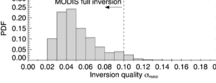
Figure 5.Statistics of the quality of the inversion. RMSE of all airborne retrievals (PDF; bin size: 0.01). Vertical dashed line shows RMSE threshold of 0.1 for MODIS full inversions.

3.7 Quality of the inversion

An exemplary inversion is performed on the snow HDRF measurement from 2 January 2014 at 08:16 UTC (θ₀= 58.9^◦). Figure 4c shows the averaged observations that are used as input for the algorithm. The inversion leads to the retrieved model parameters of 1.12 (f_iso), 0.17 (f_vol), and 0.01 (f_geo). With the calculated kernelsK_kl, the modeled HDRF is obtained (see Fig. 4d). The shapes of modeled and measured HDRF are similar; their relative difference is mostly within the range of±5 % (see Fig. 4e). The largest deviations occur in the forward scattering direction (up to 3 %) because the location of maximum is not mimicked perfectly by the modeled HDRF. However, up to viewing zenith angles of around 75^◦, the relative difference is below 1 %.

The root-mean-square error (RMSE),

σRMSE=E= v u u t

1 N−3·

N

X

l=1

(ρ_l−R_HDRF,l)²

w_l , (19)

serves as a criterion for the quality of the inversion. Only RMSEs below 0.1 are considered full inversions within the MODIS retrieval (e.g., Stroeve et al., 2005). For the example shown in Fig. 4, it is 4.0 %.σ_RMSEstrongly depends on the anisotropy of the observed HDRF. Figure 5 shows the RMSE for all airborne retrievals as a histogram, with 96 % of the retrievals showing an RMSE below 0.1. Hence, the upper bound for the uncertainty of the inversion is in the range of 10 %.

The influence of the angular sampling on the retrieval of the model parameters can be investigated using the weights of determination (WoD; Lucht and Lewis, 2000), which depend both on the angular sampling and the number of directional measurementsN. WoD (also: noise amplification fac- tors) below 1 indicate a retrieval uncertainty that is smaller than the RMSE of the inversions. Due to the largeN and consistent sampling of the viewing hemisphere, the WoD for the model parametersf_k within this study are mostly below 0.0002. For comparison, the sparse angular sampling of the reflectance measurements from MODIS observations can lead to WoD above 1, and only model fits with WoD below 2.5 are considered full inversions.

(11)

To study the stability of the inversion as a result of the uncertainties in the reflectance measurements, the stability of the retrieval of fk was studied for a 5 min flight leg over a homogeneous snow surface on 28 December 2013: the surface roughness varied between 2 and 4 cm, R_opt varied between 80 and 90 µm, and the solar zenith angle was around 55.3^◦. The inversion was performed for each individual camera picture (no averaging). The mean and SD of the retrieved model parameters along the flight leg were 1.104±0.030 (f_iso), 0.296±0.027 (f_vol), and 0.031±0.003 (f_geo). The same area was sampled five times at different solar zenith angles on 28 December 2013; the influence of θ0 on the SDs of thef_k is negligible. The mean SDs of 0.031 (fiso), 0.020 (fvol), and 0.003 (fgeo) are used as error bars for thefk

within this study.

3.8 Comparison with BRDF derived from MODIS satellite observations

The use of the RTLSR model in the retrieval of the model parameters f_k from airborne observations provides the framework to compare with satellite observations. The MODIS BRDF/Albedo Model Parameters product (MCD43A1) provides thef_k at 500 m resolution utilizing multi-date, atmo- spherically corrected, and cloud-cleared input data over a period of 16 d (Schaaf et al., 2002). Version 6 of the MCD43A1 product uses both Terra and Aqua data and is temporally weighted to the ninth day of a 16 d retrieval window, thereby putting greater emphasis on the actual day of interest than previous versions. The combination of MODIS on Terra and Aqua provides a higher number of high-quality reflectance measurements, resulting in better temporal and angular sampling. As the retrieval uncertainty increases with larger solar zenith angle, a thorough quality assessment of the satellite data is needed especially in polar regions. Stroeve et al.

(2005) compared the MODIS albedo product with in situ observations on the Greenland ice sheet and recommended only using full-inversion data (RMSE<0.1, WoD<2.5). Hence, this study restricts the satellite data to full inversions based on the quality flag information provided in the MCD43A2 product (quality flag values: 0 or 1). Lower quality-magnitude inversions would facilitate archetypal BRDF parameters to im- prove the retrieval in case of less than seven high-quality reflectance observations or poor angular sampling. The BRDF data from MODIS spectral band 4 (0.545–0.565 µm) are used as it coincides best with the green camera channel (see Fig. 3).

The MODIS data were resampled on the flight track using the nearest neighbor with respect to the great circle distance.

For the comparison, the aircraft measurements are filtered analogously: only clear-sky observations with RMSE<0.1 (96 % of total measurements), WoD<2.5 (valid for all observations), and a solar zenith angle lower than 70^◦ were used. Stroeve et al. (2005) restricted the analysis toθ₀<75^◦; however, the number of comparable observations between

MODIS and the aircraft is not reduced by the stricter condition. In fact, only 434 (21 %) MODIS observations can be compared to the 2078 airborne observations that in principle fulfill the quality requirements. For the remaining observations, no full-inversion retrieval could be performed from the MODIS observations.

4 Results and discussion

To study the influence of the solar zenith angle, the surface roughness, and the optical-equivalent snow grain size on the snow HDRF, the effects of the individual parameters need to be separated. For this purpose, several case studies were selected: (a) measurements at differentθ0(marked with red circles in Fig. 2a, five flights on 28 December 2013), (b) measurements at different surface roughness (marked with green circles in Fig. 2b, morning flight on 2 January 2014), and (c) measurements at differentR_opt(marked with brown circles in Fig. 2c, afternoon flight on 2 January 2014). The remaining two parameters were kept constant throughout the individual cases. After discussing the individual cases, the airborne observations are compared with the BRDF derived from MODIS.

4.1 Influence of solar zenith angle

The research flights with Polar 6 on 28 December 2013 were exploited to study the influence of θ0 on the snow HDRF.

Five consecutive flights were conducted in an area northeast of Kohnen Station (see red flight track in Fig. 1a).

For each flight, the snow HDRF was averaged over a 30 s segment during the easternmost flight leg; the results are shown in the top panel of Fig. 6. The solar zenith angle varied between 51.8 and 71.6^◦. As Polar 6 took identical routes throughout the flights, the respective flight leg always covered the same area. The central points of the five consecutive segments are separated by less than 1 km. Therefore, the surface roughness (retrieved from the laser scanner) of approximately 6 to 7 cm remained constant. Within the retrieval uncertainties, the same holds true for the optical-equivalent snow grain size. Ropt varied between 70 and 85 µm. This minimizes a possible influence ofRoptorlroughon the snow HDRF that would be superimposed on the effect of θ0. Cloudless conditions prevailed during the flights.

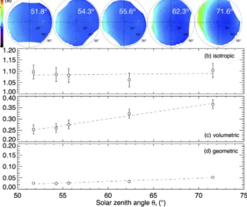
With increasing θ0, the maximum of the HDRF in the forward scattering direction becomes more pronounced (see Fig. 6). Correspondingly, the anisotropy gets larger. Figure 6 shows the dependence of thef_k on θ₀ for the green camera channel (490–585 nm wavelength).f_iso shows no clear dependence on θ₀ and varies between 1.06 and 1.10. f_geo weakly increases withθ₀from 0.03 atθ₀=51.8^◦to 0.05 at 71.6^◦. During the first three research flights,θ₀ varied only slightly. Therefore, the strongest trends are visible between flights 3 and 5. In particular,f_volincreases from 0.25 to 0.36.

(12)

Figure 6. (a)Averaged snow HDRF (490–585 nm wavelength) over 30 s segment during easternmost flight leg for the five consecutive research flights on 28 December 2013.(b–d)Dependence of the re- trievedf_kon the solar zenith angleθ₀for the five flights. The dashed lines represent linear regression fits of the parameters with respect toθ₀.(b)The isotropic weightf_iso.(c)The volumetric weightf_vol. (d)The geometric weightf_geo.

The probability of photons entering the snowpack to leave it after just a few scattering events increases for lower Sun elevation. With increasingθ₀, the reflection properties of the snow layer converge to the single-scattering properties of ice crystals. In addition, longer shadows are cast by surface roughness structures at largerθ₀. The expected increase in the anisotropy of the snow HDRF for increasingθ₀is obvious in the changing model parametersf_k and has been observed in earlier studies (e.g., Dirmhirn and Eaton, 1975; Kuhn, 1985;

Warren et al., 1998; Hudson et al., 2006).

4.2 Influence of surface roughness

On 2 January 2014, a research flight was conducted from Kohnen Station in the direction of the coastline to Neumayer Station III. The flight track is shown in Fig. 1a (green). Be- tween 08:50 and 09:00 UTC, Polar 6 crossed a sastrugi field at an elevation between 100 and 250 m a.s.l.. This fostered large variations in the surface roughness between 42 cm and 2.2 m which became distinguishable by visual observation from the aircraft. At the same time, the solar zenith angle was constant at around 55.5^◦. For these values, only little varia- tion of the snow HDRF withθ₀was found (compare Fig. 6).

The optical-equivalent snow grain size varied between 240 and 320 µm; the flight altitude remained at around 600 m above the surface, leading to a footprint of approximately 3.5 to 4.0 km. During this flight leg, 14 measurements were used to study the influence of the surface roughness on the snow

Figure 7. (a)Two examples of snow HDRF (490–585 nm wavelength) at different times during an overflight over a sastrugi field on 2 January 2014 (morning flight).(b–d)Dependence of the re- trievedf_kon the surface roughness. The dashed lines represent linear regression fits of the parameters with respect tol_rough.(b)The isotropic weightf_iso.(c)The volumetric weightf_vol.(d)The geometric weightfgeo.

HDRF. Two examples of the snow HDRF are shown in the top panel of Fig. 7.

For the smooth surfaces, the maximum in forward scattering direction is more pronounced. With increasing surface roughness, the anisotropy gets lower. Roughness structures enhance the backscatter by changing the effective angle of incidence. In addition, they cast shadows that reduce the forward scatter. The evolution of the retrieved model parameters fk as illustrated in Fig. 7 demonstrates the decreasing anisotropy:fisoandfgeoshow a slight decreasing trend, whereas, most prominently,f_voldecreases from 0.33 to 0.24 with increasing surface roughness. This is in accordance with Warren et al. (1998), who observed a reduction of the forward reflection peak due to sastrugi during tower measurements at South Pole Station. The effect of surface roughness on the BRDF has been previously investigated in observational (e.g., Grenfell et al., 1994; Hudson and Warren, 2007) and modeling studies (e.g., Leroux and Fily, 1998; Zhuravl- eva and Kokhanovsky, 2011) and is facilitated by the multi- angular reflectance data from MISR to map surface roughness over ice sheets and sea ice from space (Nolin et al., 2002).

4.3 Influence of optical-equivalent snow grain size The separation of the two parametersθ₀andl_rough showed that they influence the snow HDRF in opposite ways. Ice absorption becomes dominant in the near-infrared part of the solar EM spectrum. Hence, even though a wide variety of

(13)

Figure 8. (a) Two examples of snow HDRF (490–585 nm wavelength) at different times on 2 January 2014 (afternoon flight).(b–

d)Dependence of the retrievedf_k on the optical-equivalent snow grain size. The dashed lines represent linear regression fits of the parameters with respect toR_opt.(b)The isotropic weightf_iso.(c)The volumetric weightf_vol.(d)The geometric weightfgeo.

optical-equivalent snow grain sizes was covered during the flights (16 to 480 µm), no large effect on the snow HDRF was expected as the camera is only sensitive in the visible wavelength range (Warren et al., 1998, compare Fig. 3).

However, 32 observations between 14:45 and 15:15 UTC on 2 January 2014 (see brown flight track in Fig. 1a), depicted in Fig. 8, show a decrease offvolfrom 0.34 at 184 µm to 0.17 at 325 µm snow grain size. This is consistent with the decrease in anisotropy as visible in the averaged HDRF measurements (top panel in Fig. 8).

However, this stands in contrast to findings by Steffen (1987), who measured the bidirectional reflectance on a glacier in northwestern China for powder snow (grain size:

0.15 mm), new snow (0.5–1.0 mm), and old snow (1–3 mm) and found higher anisotropy for larger snow grains. It should be noted that the range of snow grain sizes covered within this study is significantly smaller and the footprint of the measurements is larger compared to the local study by Stef- fen (1987). Even though other parameters were kept constant during this case study (θ0: 51.3–53.4^◦;lrough: 4–7 cm; footprint: 1.3–1.7 km), effects of other influencing parameters cannot be ruled out completely. For example, Steffen (1987) reported changing ice crystal shapes between the measurements and suggested a possible influence of dust particles within the snow. This could partly explain the opposite con- clusions drawn within this study.

4.4 Parameterization of snow HDRF

The most significant effects ofθ0,lrough, andRoptwere observed on the model parameterf_vol, for which the parameterizations in terms of linear regression fits (dashed black lines in Figs. 6c–8c) are given by

fvol(θ0)= 0.0059·θ0−0.0537

(forl_rough=6−7 cm and R_opt=70−85 µm), (20) f_vol(l_rough)= −0.0656·l_rough(m)+0.3416

(forθ₀=55.5^◦ and R_opt=240−320 µm), (21) f_vol(R_opt)= −0.0009·R_opt(µm)+0.5013

(forθ0=51.3−53.4^◦ and lrough=4−7 cm). (22) The linear correlation coefficients (R²) are 0.98 (forθ0), 0.75 (lrough), and 0.68 (Ropt). Note that these parameterizations are only valid for the wavelength range of about 490–585 nm (green camera channel) and the ranges of all three parameters as given within the descriptions of the case studies.

4.5 Comparison with satellite observations

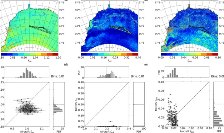
Figure 9 shows the comparison between retrievedf_k from airborne and satellite measurements for the research flight on 29 December 2013, which showed the largest amount of full-inversion retrievals for MODIS (235). The flight covered a triangular pattern southeast of Kohnen Station. The top panel shows contour plots with color coding for the three parameters as retrieved from MODIS on that day: (a)fiso, (b) fvol, and (c) fgeo. The colored circles along the flight track (black) correspond to the airborne-retrieved fk. The corresponding scatter plots between the MODIS and aircraft retrievals are shown in Fig. 9d–f. The isotropic and geometric model weights f_iso andf_geo from airborne and MODIS retrievals are in the same order of magnitude and partly agree within the measurement uncertainties.f_iso values from aircraft are slightly higher than the corresponding MODIS retrievals. This is evident from the difference in the probability density functions (PDFs) between aircraft and MODIS retrievals as illustrated in Fig. 9d–f. The comparison off_geo values shows no robust difference between airborne and MODIS retrievals. However, the lowest correlation is found for the volumetric weightsfvol.fvolvalues retrieved from aircraft range mostly between 0.1 and 0.3 and are much larger than the MODIS retrievals. The map in Fig. 9b shows that the flight covered an area where MODIS retrievedfvol

values of exactly or close to 0. In particular, this holds true for a latitudinal band around 76^◦S. Even though full inversions were reported for this area, this might still be a measurement artifact. But even for the cases with nonzero values, the aircraft retrievals lead to much higher f_vol values and, thus, larger anisotropy of the surface reflection than shown in the MODIS retrieval.

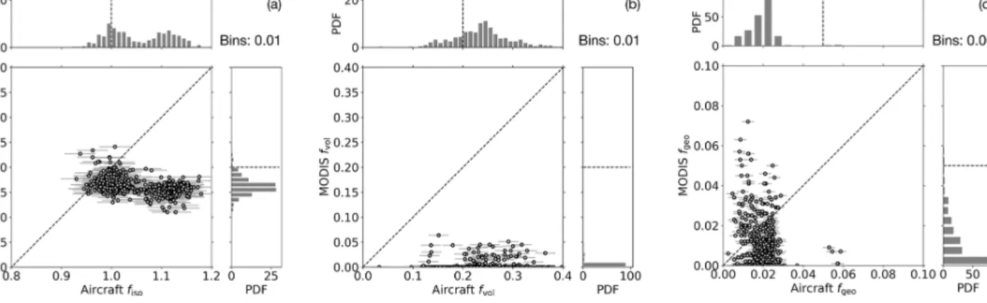
The combined scatter plots and histograms for the three model weights including all 434 observations from seven dif-