Investigation of Ultrafast Spin Dynamics by Photoemission
A thesis submitted to attain the degree of
Doctor of Sciences
(Dr. sc. ETH Zurich)
presented by
Kevin B¨ uhlmann
MSc Physics, ETH Zurich born on 26.01.1993
citizen of
Emmen LU, Switzerland accepted on the recommendation of Prof. Dr. Andreas Vaterlaus, examiner
Dr. Yves Acremann, co-examiner Prof. Dr. Michael Bauer, co-examiner
2020
The behavior of electron spins in condensed matter on ultrashort timescales is under intense investigation in theory as well as experimentally. On one hand the topic is interesting for fundamental science, on the other hand it promises big potential for applications in information technology.
In this thesis we focus on two parts of that area: the ultrafast demagneti- zation of iron and spin transport into a non-magnetic material. In both cases spin-, time- and angle-resolved photoemission spectroscopy serves as experimen- tal method. We discuss different properties as well as the implementation of this only recently applicable technique, which allows for a direct access to the spin resolved bandstructure.
The experiments on ultrafast demagnetization reveal that the spin polarization shows different dynamics during the process depending on the binding energy.
Therefore, using the magnetization as a sole quantity to describe the state of the spin system is not always sufficient on the considered timescale. We investigate the dependence of this spectrally inhomogeneous behavior on applied excitation fluence. A comparison of these results to measurements based on the widely used magneto optical Kerr effect shows a discrepancy between the optical signal and the magnetization for a short time after the excitation of the system. Finally, the evolution of the Fermi-Dirac distribution is analyzed, leading ot the observation of a spin voltage.
Spin transport is investigated in a gold/iron system, whereas the ultrafast demagnetization of the iron film serves as a source of polarized electrons. One set of experiments is performed with the excitation incident on the probed gold layer. In another it hits the iron layer through the transparent substrate. Rise and decay of a spin polarization in the gold layer are clearly visible in both cases. In a study with gold layers of varying thickness the comparison of the polarization decay times allows us to draw conclusions about the dominating relaxation pathways. It is again possible, to at least observe evidence of the presence of a spin voltage.
Das Verhalten der Elektronenpins in Festk¨orpern auf ultrakurzen Zeitskalen ist Gegenstand intensiver Forschung, sowohl experimentell wie auch in der Theo- rie. Einerseits ist das Themengebiet interessant f¨ur die Grundlagenforschung, andererseits verspricht man sich grosses Potential f¨ur Anwendungen in der Infor- mationstechnologie.
In dieser Arbeit konzentrieren wir uns auf zwei Teilgebiete: ultraschnelle Ent- magnetisierung in Eisen und Spintransport in ein nicht-magnetisches Material.
Die pr¨asentierten Experimente basieren auf spin-, zeit- und winkelaufgel¨oster Photoelektronenspektroskopie. Die Prinzipien dieser Technik, welche direkten Einblick in die spinaufgel¨osten Bandstruktur erm¨oglicht, werden diskutiert. Zu- dem wird die exakte Implementation in unserem Labor sowie dessen Eigen- schaften beschrieben.
Die Experimente zur ultraschnellen Entmagnetisierung zeigen, dass die Spin- polarisierung w¨ahrend des Prozesses je nach Bindungsenergie verschiedenen Dy- namiken aufweist. Folglich ist es auf der betrachteten Zeitskala unzureichend, den Zustand der Spins nur mittels der skalaren Gr¨osse Magnetismus zu beschreiben.
Wir untersuchen, wie sich die Dynamik verschiedener Teile des Spektrums in Abh¨angigkeit der anregenden Intensit¨at ¨andert. Ein Vergleich der Resultate aus Photoemissionsexperimenten mit jenen aus magnetooptischen Kerr-Messungen offenbart, dass das optischen Signal kurze Zeit nach der Anregung des Sys- tems deutlich von der Magnetisierung Abweicht. Eine Analyse der Evolution der Fermi-Dirac-Verteilung l¨asst uns eine Spinspannung im System beobachten.
Ultraschnelle Entmagnetisierung in einer Eisenschicht dient in den Experi- menten zu Spintransport als Quelle von polarisierten Elektronen. Gemessen wird dann der Zustand des Spinsystems in einer angrenzenden Goldschicht. Die Ex- perimente wurden in zwei Geometrien mit der Anregung von der einen oder der anderen Seite des Gold/Eisen-Systems durchgef¨uhrt. Anstieg und Zerfall einer Spinpolarisation in der Goldschicht sind in beiden F¨allen deutlich erkennbar.
Eine Studie, welche die Abh¨angigkeit des Polarisationszerfalls von der Dicke der Goldlage untersucht, erlaubt es, R¨uckschl¨usse auf die dominanten Relaxations- mechanismen zu ziehen. Es gelingt wiederum, zumindest Indizien einer auftre- tenden Spinspannung zu sehen.
Abstract iii
Kurzfassung iv
Contents v
Acronyms vii
Introduction 1
1 Methods and Setup 5
1.1 Photoemission Process . . . 6
1.2 Detection Setup . . . 8
1.2.1 Measurement of energy and angle . . . 9
1.2.2 Spin sensitivity . . . 11
1.2.3 Time resolution . . . 18
1.3 Radiation Delivery . . . 19
1.3.1 Laser system and optical setup . . . 19
1.3.2 High Harmonic Generation . . . 21
1.4 General . . . 25
1.4.1 Sample preparation . . . 26
1.4.2 Control and data acquisition . . . 27
1.4.3 Data processing . . . 28
2 Demagnetization Experiments 33 2.1 Introduction . . . 34
2.2 Sample . . . 38
2.3 Remarks on results . . . 39
2.4 Dynamics at fixed energies . . . 41
2.4.1 Fitting function . . . 41
2.4.2 Spectrally inhomogeneous depolarization . . . 42
2.4.3 Fluence dependent study in the valence band . . . 45
2.4.4 Fluence dependent study at the Fermi energy . . . 46
2.4.5 Field of view in magneto optical Kerr effect (MOKE) . . . 48
2.5 Spectral scans . . . 50
2.5.1 Exchange splitting reduction versus band mirroring . . . . 51
2.5.2 Evolution of the Fermi-Dirac distribution . . . 54
2.5.3 Dynamics above the Fermi energy . . . 60
2.6 Summary and conclusion . . . 61
3 Spin Transport Experiments 63 3.1 Introduction . . . 64
3.2 Samples . . . 67
3.3 Remarks on the results . . . 70
3.4 Dynamics at the Fermi energy . . . 70
3.4.1 Front pump geometry . . . 70
3.4.2 Back pump geometry . . . 72
3.5 Dynamics in the valence band . . . 75
3.6 Evolution of the Fermi-Dirac distribution . . . 78
3.7 Summary and conclusion . . . 80
Bibliography 83
List of Publications 99
Curriculum Vitæ 101
Acknowledgments 103
STARPES spin-, time- and angle-resolved photoemission spectroscopy STT spin transfer torque
SPLEED spin polarized low energy electron diffraction ARPES angle-resolved photoemission spectroscopy HWP half wave plate
HHG high harmonic generation BZ Brillouin zone
DOS density of states UV ultra violet
XUV extreme ultra violet
IR infrared
TOF time of flight
HEA hemispherical energy analyzer MCP microchannel plate
SOC spin orbit coupling UHV ultra high vacuum
FWHM full width half maximum FEL free electron laser
BBO beta-barium borate
MOKE magneto optical Kerr effect 3TM three temperature model
M3TM microscopic three temperature model LLB Landau-Lifshitz-Bloch
RKKY Ruderman-Kittel-Kasuya-Yoshida
mSHG magnetization dependent second harmonic generation
From static magnetism to ultrafast spin dynamics
In every day life, magnetism is usually directly encountered in form of permanent magnets, i.e. ferromagnets with high Curie temperature. Nowadays of great technological importance is the long lasting magnetization for data storage in magnetic hard drives. In this static or quasi-static case the magnetization M~ is aligned parallel to a strong enough magnetic field H. Note that this field~ can also include internal contributions stemming for example from the exchange interaction or spin orbit coupling (SOC).
We now leave the static case by first considering a non-parallel configuration of a magnetic moment m~ and a field H. Now~ m~ experiences a torque ddt~L given by:
dL~
dt =m~ ×µ0H~ (1)
with the permeability of the vacuumµ0. With the introduction of the gyromag- netic ratio γ that links magnetic moment to angular momentum we can express the torque as a change of magnetic moment. If we then also take the average of
~
m per volume, we arrive at a differential equation for the magnetization:
dM~
dt =−γ ~M ×H~ (2)
As the differential is proportional to the cross product of magnetization and field, it does not lead to an alignment of the two but causes a precessional motion
at field strengths around one Tesla.
However, as mentioned above our experience tells us that M~ is aligned to H. This is achieved by the introduction of a phenomenological damping term~ αMM~ × ddtM~ that forces the magnetization along the field. The resulting equation is called the Landau-Lifshitz-Gilbert equation [1, 2]:
dM~
dt =−γ ~M ×H~ +α M~
M × dM~
dt (3)
As the magnetic moments that lead to a magnetization are carried by electrons, there is also the possibility to manipulate magnetization by a spin current. This effect can be considered as an effective torque, therefore it is known as spin trans- fer torque (STT) [3]. The spin currents are usually created by the transmission of an electrical current across the interface between a ferromagnet and a nor- mal metal. The transport properties of this interface lead to a polarization of the passing electrons. This puts the field in the timescale of electronics that is slightly below the nanosecond range. In this context it is also worth mentioning the material class of topological insulators that host a permanent spin current in their surface state.
This work considers the case of further increased temporal resolution and in- tense stimuli. Under these conditions the effect of ultrafast demagnetization, i.e.
a partial loss of magnetization in less than a picosecond, is observed. Since this effect can serve as a source for spin currents on the same time scale, it also enables spintronics in that range. The emerging field, often called femtomagnetism, has attracted great interest for several reasons elaborated closer in the next section.
It does not come as a big surprise that equation 3 is not sufficient to describe the observed dynamics. Nowadays several partially competing or redundant theoret- ical frameworks are around, the most prominent ones are presented in sections 2.1 and 3.1.
Motivation
We investigate spin dynamics on the femtosecond timescale in condensed matter by photoemission. Why is the topic worth the effort? And what advantages brings the use of this very delicate measurement technique?
First of all, the field of ultrafast spin dynamics is quite interesting from a pure scientific point of view: We can learn about the interaction mechanisms between the spins and other degrees of freedom - for example charge and lattice - in a system that is driven far out of equilibrium. The presented experiments deliver further information towards a more general understanding of the principle mechanisms behind ultrafast demagnetization, which is a long-lasting challenge within the field. Another interesting point is the effect of inter- and surfaces, i.e. broken translational symmetry along one direction, on the lifetime of a spin imbalance in a non-magnetic material.
We have chosen spin-, time- and angle-resolved photoemission spectroscopy (STARPES) for our experiments since it offers the opportunity to measure spin polarization in a rather unambiguous way. Furthermore one also obtains addi- tional information about the electronic states of the sample under investigation at the same time, as discussed in chapter 1. Both of these points make the technique a valuable addition to other, due to their easier implementation more commonly used methods such as magneto optical Kerr effect (MOKE) or magnetization dependent second harmonic generation (mSHG).
Possible applications that motivate the pursuit of this field of research mainly lie in information technology. For the demagnetization experiments presented in chapter 2 the major incentive is the acceleration of the writing process in magnetic storage media (hard drives). Changing a bit means inverting the mag- netization locally. For now this is done by the application of a magnetic field that causes the motion of the magnetization governed by equation 3. This way, switching times are typically in the range of nanoseconds [4]. The idea is to decrease this time using the ultrafast demagnetization effect. First, the magne- tization is strongly reduced within picoseconds and recovers as under an applied field in the other direction. Strongly related to that is the concept of heat as-
Hc. Excitation by a laser pulse is than used to locally decrease the medium’s coercivity such that its magnetization can be changed [5].
Transport of spins, investigated in chapter 3, is the key element of spintron- ics. Most prominent example of this field is the giant magnetoresistance (GMR), working principle of modern magnetic hard drives [6, 7]. However, spintronics is not only promising for long term data storage but also for data transmission and processing. The change from charge - as in classical electronics - to spins can offer advantages as dissipationless information transfer or great reliability in a radioactive environment, which is an issue in space technology. An application that was recently commercialized (Everspin Technologies) is magnetic random access memory (MRAM) [8], which is in contrast to its conventional counterpart non-volatile. MRAM also offers faster writing speeds and more write cycles.
The last point from the application side - often forgotten - in favor for the con- duction of the presented experiments is the improvement and better understand- ing of the applied measurement technique. As mentioned, it is rather delicate but also extremely powerful as it delivers a lot of information at the same time in a direct way. Therefore, we think that STARPES bears great potential for the application in other fields where the electronic structure including its spin state is crucial, e.g. topological insulators.
Methods and Setup
Before we discuss experimental data and the conclusions thereof, we shall understand how to obtain them in this chapter. The results presented in this work were obtained by spin-, time- and angle-resolved photoemission spec- troscopy. This technique gives direct access to the dynamics of the spin re- solved band structure and the corresponding electron occupation. First, the photoemission process itself is explained in limited theoretical depth. The sections on the detection setup and the creation of the radiation for photoe- mission contain both, basic concepts and the actual implementations. The last part focuses on practical details concerning the experimental work and data analysis.
1.1 Photoemission Process
In photoemission a formerly bound electron is emitted from a system due to absorption of one or several photons. In solid state physics the process is often described in terms of the three-step model [9]:
1. Excitation of the electron in an unoccupied state by the photon 2. Transport of the electron to the surface
3. Escape of the electron into vacuum
This model is a strong simplification of the very complex evolution of the many body wavefunction of the macroscopic system, which the solid is. However, it is very useful as it allows for meaningful interpretation of experimental results. A more accurate description is the one-step model [10]. Due to its higher complex- ity and the fact that it delivers no further insight in the following, we will not cover it.
What information about their initial state and therefore the electronic structure of the solid do the emitted electrons carry? First, we consider energy within the three-step model: the electron gains the energy of the absorbed photonEph =~ω in the first step. During the second step no interaction takes place (which is a severe simplification made in the model). In the final step the electron has to overcome a potential step between the solid and the vacuum, the so-called workfunction Φ, a material specific constant. With this information we can derive an expression for the binding energy EB measured from the Fermi level EF:
EB =Ekin+ Φ−EP h (1.1)
Note that we use the convention of negative binding energy for bound states.
Once we know the energy (wavelength) of the radiation used in the experiment as well as the work function, we can learn about the spectral distribution of the electronic states in the solid i.e. the density of states (DOS).
However, it is by far not trivial to completely determine the DOS in the solid from the energetic distribution of the emitted electrons, as two major points have not been in consideration so far. First, the probability that at a certain
binding energy an electron absorbs a photon does not only depend on the DOS but also on the actual form of the electron’s wavefunction, the photon’s energy and polarization as well as the density of unoccupied states the electron can be excited in [11–13]. Second, there is a chance for the electron to scatter on its way out, which is again dependent on the specific state the electron is in during the second step. The same holds true also for the transmission probability into vacuum. The scattering of the primary electron on its way to the surface also frees additional electrons. These secondary electrons can scatter again, leading to the so-called cascade of secondary electrons [14]. Furthermore, it is experimentally often not possible to detect electrons over the whole momentum range as we will see below.
The energy dependence of the scattering probability during the second step of photoemission results in a typical escape depth for a certain photon energy [15]. This can be of use, as it allows to tune the surface or bulk sensitivity of an experiment by varying the wavelength of the radiation.
Since we work with ultra violet (UV) radiation, the photon momentum is very small compared to the momentum of the electron and can be neglected in the process in good approximation [16]. Due to the translational symmetry along the surface, the respective components of the momentum ~pek are conserved during the whole process [17]. The component orthogonal to the surface pe⊥ changes during the third step. To get information aboutpe⊥ of the initial state one often assumes parabolic band dispersion and back-calculates it from the energy and
~
pek. In solid state physics a common convention is to work with the reciprocal vector~ke that is related to the momentum in a linear fashion:
~
pe =~~ke (1.2)
The dispersion of the free electron implies a highest possible absolute value of the reciprocal vector parallel to the surface for a given photon energy and workfunc- tion, the so-called photoemission horizon. It is the |~kek| of an electron that was originally at the Fermi level and is emitted with vanishing momentum component perpendicular to the surface:
kkmax =
p2me(Eph−Φ)
~
(1.3)
Therefore, the photon energy determines not only the interval in energy but also the size of the reciprocal space that is maximally accessible in a photoemission experiment.
Another aspect to consider is the spin of the electrons. If an electron undergoes the photoemission process without scattering, its spin is conserved. However, the probability for all three steps of photoemission can be spin dependent [18–
20]. The matrix element for the excitation is influenced by the polarization state of the radiation, which is the basis for several measurement techniques, for instance x-ray magnetic circular dichroism (XMCD) [21]. The behavior during transmission, i.e. the spin dependent scattering probability, and escape influence the polarization of the secondary electrons [19].
Thus, in principle the emitted electrons carry all the information necessary to reconstruct the band structure and electron occupation of the material under investigation. However, the considerations above make clear that this informa- tion cannot be retrieved directly. We will see how to actually measure these quantities in the next section as well as how to add the temporal dimension.
1.2 Detection Setup
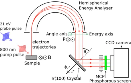
It is our goal to determine an electron distribution in the four dimensions energy, momentum, spin and time. The former three need to be detected for the emitted electrons, the latter one is controlled and set to desired values. A schematic overview of the complete detection setup including incoming radiation for exci- tation and emission is shown in figure 1.1.
Although the photoemission process itself can take place under any condition, photoemission experiments require an ultra high vacuum (UHV) environment.
Air absorbs all emitted electrons (in this case already the radiation used for emission) and prevents the build up of high voltages necessary for detection and the electrostatic optics. Furthermore, samples degenerate completely in less than a second under ambient conditions.
Figure 1.1: Schematic overview of the STARPES detection system. The sample is excited by the pump pulse and after a set delay the probe pulse emits elec- trons. These travel through the HEA, which sorts them according to energy and emission angle. An electrostatic lens system guides them to the Ir(100) crystal, where they undergo a spin dependent diffraction. Finally the are detected by the MCP - phosphorous screen - camera assembly.
1.2.1 Measurement of energy and angle
In one approach to determine the emitted electrons’ energies a static electric or magnetic field, that sends electrons on different trajectories depending on their energy, is applied, s.t. they end up on different spots on a detector. These dispersive methods typically have two main drawbacks: First, it is only possible to measure one component of the electron’s momentum at once. Second, in most cases a lot of emitted electrons are not sent to detection. A part of them are filtered out either because they have an energy that is out of the transmitted interval or because their initial momentum along the energy dispersive direction of the analyzer disturbs the energy-position relation too much.
Another family of techniques is based on the time of flight (TOF) from emis- sion to detection. These methods do not suffer the issues mentioned before or at least only to a smaller extent. Since time measurements are only possible with well defined starting points, they are applicable exclusively for pulsed photon
sources. In addition, TOF systems, especially their detectors, are typically more complex as they have to be able to detect not only the position of an incident electron but also the time of its arrival.
Resolution in reciprocal space is achieved by using a field geometry that maps emission angle - to be more precise the pair of polar and azimuthal angle φ and θ as indicated in figure 1.2 - onto detector position. To gain full band structure information with a dispersive setup, one needs to rotate the sample relative to the detection system, as it records only a certain slice of the emission cone.
The original ~kk can be calculated with the measured emission angle and the kinetic energy by:
~kk =
√2meEkin
~
sin(θ)
cos(φ) sin(φ)
(1.4) where me is the free electron mass.
Θ
Φ
M
Figure 1.2: Schematic of the photoemission geometry. The area in blue depicts a typical acceptance window of the HEA. The double arrow labeled M indicates both, the axis along which the sample can be magnetized as well es the spin sensitive direction of the setup.
In our laboratory a hemispherical energy analyzer (HEA) (Phoibos, Specs Inc.) sorts the emitted electrons according to kinetic energy and one direction of emis- sion angle. This device consists of two concentric hemispheres between which
a voltage is applied, such that the kinetic energy of electrons and their angle along the dispersive direction lead to different elliptical trajectories as depicted in figure 1.1. Electrostatic optics that guide the electrons into the dispersing part give the possibility to de- or accelerate them prior to the sorting process.
The detector is an assembly of a microchannel plate (MCP) that amplifies incoming electrons by up to six orders of magnitude, followed by a fluorescent phosphorus screen and an actively cooled CCD camera.
1.2.2 Spin sensitivity
It is challenging to add sensitivity for the spin polarization P of emitted elec- trons to an existing angle-resolved photoemission spectroscopy (ARPES) setup.
Earlier techniques such as the widely used Mott scheme [22], where spin orbit coupling results in a spin dependent angular distribution after high energy scat- tering (typically 50 keV) on a gold foil distort the trajectories of the electrons in a way, that angular and spectral distribution cannot be inferred. Therefore, it is usually necessary to preselect a certain window of energy and angle of the emitted electrons which will then result in one single measurement point. Furthermore, Mott scattering suffers from very low efficiency.
Measuring the spin polarization without losing spectral and angular informa- tion has only recently become possible thanks to the advance of two dimensional low energy scattering methods [23]. In this case spin polarized low energy elec- tron diffraction (SPLEED) on an iridium(100) crystal under an angle of 45◦ is applied [24, 25]. The probability for an electron to be reflected on the analyzer crystal is spin dependent due to the strong SOC, a relativistic effect, in the heavy element Ir [26]. The setup is sensitive to the projection of the spin perpendicular to the plane defined by the electron trajectory (out-of-plane in figure 1.1). The scattering energy is determined by the voltage applied to the crystal. In our case the scattering energy was around 6 eV.
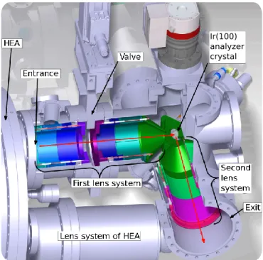
The iridium crystal is smaller than the output of the HEA and the sensitive area of the detector. In addition, the electrons have to decelerate before scattering without distorting of their distribution. Therefore, an electrostatic lens system
is needed from HEA output via Ir crystal to the detector. The whole assembly as designed by Gerd Sch¨onhense in its vacuum chamber is illustrated in figure 1.3.
Ir(100) analyzer crystal
Figure 1.3: CAD drawing off the spin analyzer assembly.
The configuration of the electrostatic system including settings of the HEA and the iridium crystal, further referred to as lens mode, critically affects the performance of the detection system. The three main requirements for a lens mode are
• Spin selectivity
• Imaging of HEA output onto detector
• Portion of transmitted phase space
Including deflectors such a lens mode consists of more than 20 voltages in a possible range of plus minus a few hundred volts. Although it takes a lot of time to manipulate all these values until a good configuration is found, it is surely worth the effort: Going from a mediocre mode to a more elaborate one can cut
half the measurement time necessary for a certain data quality or bring features of the band structure in the field of view that were not visible before.
The spin selectivity is in general rather simple to achieve, it is mainly controlled by the voltage applied to the Ir crystal that together with the pass energy of the HEA defines the scattering energy. The effect of a change in crystal voltage on the electron trajectories can be compensated to a great extent by an adjustment of the voltages applied to the neighboring elements. Therefore, spin selectivity can by optimized without the need to manipulate the whole electrostatic config- uration. The imaging properties and the transmitted phase space however have proven to be very demanding as they are affected by every single voltage. Even worse, they often react in opposite ways when moving around in the parameter space. E.g. increasing the interval of reciprocal space that is delivered onto the detector typically smears out features in the center of the transmitted window or introduces strong deformations. It is favorable to not only have imaging trans- mission from HEA to detector but also on the parts to and from the analyzer crystal. This way one gets a sensitive tool to monitor the state of the crystal. It also facilitates the search for new lens modes since the part before and after the SPLEED can be manipulated quite independently.
Figure 1.4: Detected image for a powerful lens mode under benchmark condi- tions. The stripes originate from electrons with equal angle of emission, set by an aperture with parallel slits in front of the HEA.
Manipulation of a lens mode is only reasonable if its performance regarding all three aspects can be monitored while doing so. For this an aperture with regular thin slits is placed in front of the entrance of the HEA. It is oriented such that only electrons with certain emission angles along the energy sensitive direction of the system are transmitted. This results in a pattern of equally spaced, parallel, thin stripes along the energy direction at the output. Ideally the same pattern is observed on the detector. In order to see the effect of applied changes in real time, the fluence of generated electrons needs to be significantly higher than during the photoemission experiment. Therefore, we use the secondary electrons produced by an electron gun, firing with an acceleration voltage of 1.5 kV onto a small spot on the sample.
Figure 1.4 displays the image on the detector in this benchmark configuration for one of the best available lens modes, which was also used measuring a lot of the presented data. Although the lines of constant angle are not perfectly paral- lel, their distortion is small, smearing out is very limited and all lines are clearly distinguishable. Hence the reconstruction of the actual electron distribution is feasible.
Our measurements require the magnetization of the samples to be set along the sensitive direction of the SPLEED process. This is enabled by a stray field coil pair without a core connected to a pulsed voltage source as described in [27].
With this setup the experiment can be performed in the absence of additional magnetic fields that distort the emitted electrons’ trajectories. A metal plate on the same level as the photoemission spot completes the whole assembly directly surrounding the sample and is depicted in figure 1.5. The plate acts as a potential plane that homogenizes the electric field acting on the emitted electrons. It has star-shaped cut-outs in front of the coils to suppress eddy currents.
The spin information is acquired by recording two data points (as we work with a 2D-detector, these are images) with opposite sample magnetization under otherwise identical conditions. We can label the recorded distributions of elec- trons in energy and angle as p and m (plus/ minus, magnetization direction of sample up/ down). The measured asymmetry A is then defined as:
A= p−m
p+m (1.5)
Figure 1.5: Front (a) and back (b) view on the direct surrounding of the sample in the measurement chamber including the stray field coil pair and a metal plate as potential plane. The big circular cut through sample and plate is virtual and only for better visibility. Reprinted from [27]
Because SPLEED is not fully spin selective, i.e. electrons with the unfavorable spin direction for the process still have a finite reflection probability too, this value does not yet reflect the actual spin polarizationP of the emitted electrons.
Therefore, we label the directly measured data as plus and minus (pand m) and the ”true” values as up and down (s↑ and s↓). The ratio between asymmetry and spin polarization is the Sherman factor S:
P = s↑−s↓
s↑+s↓
= A
S (1.6)
whereupand down denote the two spin distributions in the emitted electrons.
The Sherman factor depends on the exact scattering energy and angle. Since these two quantities are not constant over the whole area of the crystal, S is in principle a function of the position on the crystal that is different for every lens mode. However, we use a constantS for the calculation of the polarization. This is justified by the binning in energy and momentum (see section 1.4) and the way we scan over the photoelectron spectrum. With equations 1.5 and 1.6 we find a formula to disentangle the measured data into the original distributions (up to a constant factor):
s↑ =p−1−S
1 +Sm (1.7)
s↓ =m− 1−S
1 +Sp (1.8)
The Sherman factor of our setup was determined to be around 0.5 with varia- tions depending on the exact lens mode. This calibration relies on the measured asymmetry of low energy secondary electrons (Ekin = 1 eV) stemming from an iron sample excited by the electron gun which is then compared to the values of the actual spin polarization found in [28, 29].
The portion of electrons that head to the detector after diffraction is reported to be around one percent under similar conditions [30]. With the Sherman factor and this effective electron reflectivity R one can determine the figure of merit F given byF =S2·R to be 2.5·10−3. F is well suited to quantify the performance of a spin detector since it is directly inversely proportional to required integra- tion time (for a certain data quality). Values for Mott-based polarimeters are typically three orders of magnitude lower.
The described procedure only works for ferro- and ferrimagnets. If other sam- ples with nontrivial spin structure shall be investigated, it is not possible to achieve contrast by switching the magnetization. Luckily there is the possibility to change the scattering energy instead, such that one data point is taken with high spin sensitivity and the other with none or even inverse one. However, if the scattering energy is altered, also the imaging properties from HEA to detector are changed. This is an issue, since the difference of the obtained images is used for further analysis. Some distortions can be corrected by morphing the images, but this is only feasible for rather small distortions. This puts restrictions on the difference between the two used scattering energies. Therefore, we have chosen to work with a second scattering energy without spin sensitivity close to the one used in the normal procedure.
In principle one could base a measurement sequence on the rotation angle of the crystal around its symmetry axis, denoted as Φ in figure 1.1, because rotat- ing the crystal has the same effect on the deflection properties as changing the scattering energy in a limited window. It is therefore possible to go from high
spin sensitivity to none by altering this angle. This has not been implemented so far because the rotation can only be set by hand and there is concern that a very frequent motion of the crystal damages wiring or mechanics. Furthermore, imperfections of the analyzer crystal lead to artifacts in the obtained spin polar- ization
The elastic mean free path of only a few angstrom in the respective energy range [31] causes SPLEED to take place in the few uppermost atomic layers of the iridium crystal. This implies the necessity of an extremely clean surface.
The Ir is prepared for operation in two steps: Several flash annealing cycles at roughly 1200 K in an oxygen atmosphere of 4.5·10−8 mbar remove carbon from the surface. Subsequent high temperature flashes up to 2200 K free the surface from remaining oxides and oxygen [32]. If necessary this procedure is repeated several times.
After preparation the performance of the crystal decreases even in a<10−10mbar environment within a few hours down to around 50% of the original sensitivity.
This increases the necessary integration time significantly and imposes frequent measurement brakes of several hours.
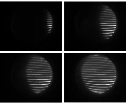
Fortunately the fast degradation of the iridium surface can be prevented by a protective single monolayer of gold on the crystal [30, 33]. In order to get that exact one monolayer coverage all over the crystal, a few layers of gold are deposited from a Knudsen type evaporation cell with a deposition rate of around half a monolayer per minute right after the regular preparation procedure. Then all but the last one are removed by heating of the crystal to around 900◦C for half an hour. The procedure is based on the fact that gold is stronger bound to the iridium surface than to itself. The progress of the removal can be checked under normal experimental conditions with a suiting lens mode as SPLEED (or in this case also just LEED) can show clear contrast between one, two or more than two layers of coverage. The reduction of the excessive gold is visible in figure 1.6.
Between individual images the crystal was heated for five minutes. The darker part of the observed island marks a region of three or more monolayers of gold, the border around it consists of two layers. The protection increases the life time of a freshly prepared crystal form hours to at least months (we never observed
degradation before we had to prepare the crystal due to other reasons such as chamber venting or bake-out of another part nearby).
Figure 1.6: Shrinking of the region of two or more monolayers of gold. Between the separate images the crystal was heated for five minutes.
1.2.3 Time resolution
If we want to see the evolution of a system after excitation we can either use a fast detector, that delivers the desired temporal resolution, and measure every- thing at once. The other option is to use a (at least on the relevant time scale) slow detector in combination with a short probe, (analogous to a flashlight in photography) whose duration then determines the resolution. Hence we mea- sure in a stroboscopic manner with varying delay between the excitation and the probe. This second measurement technique is referred to as pump-probe and it is widely applied in ultrafast science. Its only requirement is that the investigated process can be repeated many times since only one point in time is obtained per measurement. The processes considered in this work typically happen on a femtosecond (fs) to picosecond (ps) timescale, where no detectors are available.
Hence all presented experiments are based on the pump-probe scheme.
Excitation (pump) and probe are both implemented as light pulses of around 20 fs full width half maximum (FWHM) duration, setting a lower limit of the overall time resolution into the same range. Since we are using light, the delay between pump and probe can be changed via the optical path difference of the
two beams. This distance can easily be manipulated by a mechanical stage whose positioning precision allows even for sub fs control. Pump and probe originate both from the same laser system. Therefore, the timing jitter between the two is negligible. In the schematic overview in figure 1.1 varying delay would be illus- trated as changing the distance between the two pulses. A detailed description of the laser system, the optical setup and the generation of the pulses used for photoemission can be found in section 1.3.
1.3 Radiation Delivery
The driving machine behind the presented scientific work is, as for the majority of today’s ultrafast (sub ps) science, a pulsed laser system. Short pulses of light facilitate experiments with a time resolution in the range of the pulse duration.
Furthermore, the brevity of the pulses often imply high peak powers, giving the possibility to harness non-linear effects with usually unreachable efficiency and up to otherwise inaccessible order. A typical example for such an effect is the high harmonic generation (HHG) that serves as a source of UV radiation for photoemission in our laboratory.
1.3.1 Laser system and optical setup
The ultrashort laser pulses are provided by a titanium sapphire laser system. A passively modelocked oscillator (Vitara, Coherent Inc) seeds a regenerative am- plifier (Legend Elite, Coherent Inc) that works on the principle of chirped pulse amplification [34]. This means that pulses are strongly dispersed for amplifica- tion in order to avoid damage in any optics and subsequently recompressed. The specifications of both, the oscillator and the amplifier are summarized in table 1.1.
First the provided beam is split into two branches with variable relative inten- sity by a rotatable half wave plate (HWP) and a polarizer. One partial beam is used for the generation of more energetic radiation (described in detail in the next section) that finally emits electrons from the sample and is therefore called the probe beam. The other is directed over a delay stage that enables us to scan over the pump probe delay, towards the sample. A peculiarity of the used
Oscillator Amplifier Repetition Rate 80 MHz 10 kHz
Pulse Duration 10 fs 20 fs Average Power 550 mW 12 W
Pulse Energy 7 nJ 1.2 mJ
Peak Power ∼1 MW ∼100 GW
Center wavelength 800 nm 800 nm
Polarization p p
Table 1.1: Typical specifications of the oscillator and the amplifier.
laser system is that it has two separate compressors for the two branches. This enables dispersion compensation for the individual beam paths. Furthermore, it is possible to control the pump pulse duration without affecting the probe. A sketch of the setup is depicted in figure 1.7.
Beam: 800nm 400nm 21eV BBO Al foil Polarizer Mirror: 800nm 400nm 21eV HWP Lens Si waver
to sample Mirror chamber
HHG Compressors
Oscillator
Amplifier
Delay stage
Figure 1.7: Scheme of the optical setup. The oscillator provides seed pulses for the amplifier whose output is split and then recompressed. The pump beam is led over a delay stage. The probe is frequency doubled in a BBO crystal.
The emerging 400 nm light is focused in argon, generating UV radiation. The combined beam passes elements for filtering and refocusing before entering the measurement chamber.
1.3.2 High Harmonic Generation
Since its discovery in the late 80s [35] HHG from ultrashort laser pulses has become a widely used tool for the study of ultrafast processes. The reasons for their success make them also very suitable for laboratory-based time resolved photoemission experiments:
• Possibility to produce pulses with a duration down to the attosecond range [36]
• Depending on specifications of the driving laser access to photon energies from the UV up to soft X-rays [37]
• High temporal and spatial coherence within the pulses
• Intrinsic synchronization and even coherence with laser system that is often also used for another purpose in the experiment (e.g. excitation or streaking of emitted electrons)
• A HHG setup can be very small (tabletop), especially compared to their (partial) alternatives, free electron lasers (FEL) or slicing sources at syn- chrotrons, which have overall sizes in the km range.
• Implementation is relatively - again compared to the above mentioned alter- natives - easy and, if the short pulse laser system is already present (which it was in many laboratories specialized in ultrafast science), affordable.
In the prototypical HHG setup a single-color, linearly polarized pulsed beam with central wavelength λ0 is focused into an atomic gas. This produces a frequency comb of odd harmonics of the fundamental photon energy. Their spectrum stretches over the plateau, where the intensity of all peaks is almost constant, up to the cutoff, where the intensity decreases over several orders of magnitude within a few harmonics. Variations of that basic scheme are possible and allow for a change of the properties of the generated radiation: A bichro- matic driving beam that includes the second harmonic or a target that brakes full rotational symmetry - it may also be solid or liquid - can lead to even har- monics [38, 39]. Certain combinations of generating field and target molecules are reported to deliver a circularly polarized output [40, 41].
Similar to photoemission the complex process of HHG, that involves multiple particle wavefunction evolution in strong fields, can be described surprisingly well by a simple semi-classical three step model [42].
1. Tunnel ionization of an atom in the strong field of the laser pulse, where the atomic potential is tilted strongly enough to become a barrier with finite tunneling probability.
2. Acceleration of the electron in the varying electric field, first away from and then back to the ion it stems from.
3. Recombination with the ion. The potential drop and the built up kinetic energy are released as broadly distributed radiation up to the highest pos- sible photon energy that is the sum of the two.
The whole process can start at any half cycle of the driving pulse, if the atom has not been ionized so far. Since there is a macroscopic number of atoms in the target, this leads to emission at twice the laser frequency (not to be mistaken with the repetition rate of the laser). The full rotational symmetry of the atomic gas suppresses any systematic difference between radiation generated at the two different half wave directions. Altogether these multiple, coherent bursts of emission give rise to the observed spectral structure that only contains odd harmonics. This also explains, why a single oscillation driving pulse produces just a very broad spectrum without any additional structure.
Based on the three step model one can also determine the highest available photon energy dependent on wavelength and peak intensity. It can be shown that the cutoff evolves linearly with the intensity and quadratic in λ0, i.e. the energy of the generated photons can be the higher, the lower the energy of the incoming ones is.
The three step model in its simplest form as presented above reaches its lim- its when it comes to the description of the driving wavelength’s influence on the efficiency and parameter optimization. In the former case multi-photon photoion- ization plays an important role, the latter crucially depends on phase matching in the macroscopic target. It turns out that the efficiency is proportional to something between the fifth and the sixth power of λ0 [43]. For parameter opti- mization ionization of the target and the thereby induced changes in refractive
indices for the involved wavelengths need to be taken in account. Experimentally the phase matching is manipulated via the gas pressure in the target.
The generated radiation, especially the one in the UV and extreme ultra violet (XUV), can undergo significant absorption and - in particular important for attosecond science - dispersion in the target. Therefore, it is desirable to have a steep gradient in gas pressure after the generation region. This is achieved in one of the following ways [44], listed in the order we have implemented them:
1. Focusing of the laser in a thin capillary that then acts as a waveguide and a containment of the target at the same time
2. Confinement of the gas to a cell in the optical path with openings that just match the beam size
3. Crossing of the driving beam with a small gas jet perpendicular to the beam
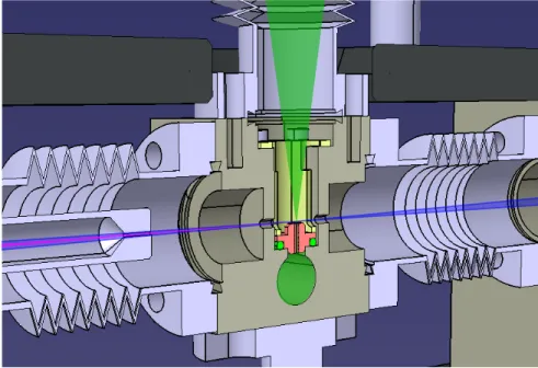
In our setup the third option has proven to work best. Its implementation can be seen in figure 1.8. The driving beam enters the chamber from the right through a window at Brewster’s angle. The target gas argon is provided from the bottom and enters the generation chamber, where the beam is in focus, through a capillary with a diameter of 75µm in form of a jet. The majority of the gas is pumped through the upper exit of the chamber by a scroll pump. The additional small confinement on the optical path serves as a differential pumping stage to lower the argon pressure, thereby decreasing the absorption of high harmonics.
Finally, the beam enters the next vacuum chamber.
The central part, the generation chamber, is connected by bellows to the re- maining system and attached to a translational stage with two degrees of freedom perpendicular to the beam direction. This way the Ar jet can be positioned op- timally relative to the laser focus. Changing the beam path is not an option as it is already well defined by the small apertures on its way. In this setup optimization of the source is possible without an optical realignment.
As mentioned above HHG has broad range of specifications depending on the detailed implementation. What properties are most favorable (and feasible) for our experiment, i.e. spin-, time- and angle-resolved photoemission spectroscopy?
Figure 1.8: CAD cut through the HHG source. The driving beam (blue) enters from the right, is in focus right above the argon (green) inlet, where the UV radiation (purple) is produced. A pumping stage lowering the residual Ar pres- sure follows. The generation chamber, the central block, can be moved for ideal positioning of the jet relative to the beam.
• Resolution in energy and momentum forces us to isolate one harmonic for photoemission, otherwise we measure a superposition of several electron distributions. A larger separation of the individual harmonics in the spec- trum simplifies the selection of a single one.
• In the spin filtering process the number of electrons is reduced by roughly two orders of magnitude [30], making a high efficiency necessary for rea- sonable integration times in the experiment.
• We are mainly interested in the dynamics of the valence band, implying a minimal photon energy. It has to exceed the sum of a typical valence band width of around 10 eV and workfunction in the range of 5 eV by a few eV.
The additional energy is needed in order to avoid coverage of significant features in the electron spectra by the cascade of secondary electrons.
As we do not aim for time resolution below tens of femtoseconds, the pulse (train) duration can be blissfully ignored, it is shorter than the driving and the pump pulse anyway.
These demands in combination with the opportunities the laser system offers and advice given by Michael Bauer led us to a design where the second harmonic of the laser beam, shown in blue in figure 1.7, drives the HHG [45, 46]. This way the process is efficient enough to observe a distortion of the photoelectron distribution due to the Coulomb repulsion of its own charge density, the so- called space charge effect [47, 48]. Cutting the driving wavelength half also doubles the line separation in the radiation spectrum, making the isolation of a single harmonic much easier. The seventh harmonic at 21 eV, chosen for our experiments, satisfies the above stated requirement for the photon energy and is below the cutoff under these conditions.
After generation the beam has to be refocused and filtered on its way to the sample. These tasks are performed in a separate vacuum chamber at a typical operational pressure of 10−5 mbar, referred to as mirror chamber in figure 1.7.
First the radiation hits a silicon waver under Brewster’s angle for light at 400 nm of 80◦, absorbing most of the driving beam. The reflectivity for the UV is close to unity at gracing incidence. This step is not compulsory as the subsequent elements in principle could also filter out the 400 nm light. Therefore, it was originally not a part of the setup. However, without this strong attenuation the driving beam is powerful enough to introduce damage on its further way, where replacement is time consuming and expensive.
Two concave Bragg mirrors designed for reflection of 21 eV radiation under 5◦ angle of incidence first collimate the beam and then focus it onto the sample. At the same time they act as a filtering element. A 75 nm thick, freestanding alu- minum film almost fully blocks all remaining radiation below 15 eV and protects the UHV environment in the following measurement chamber.
1.4 General
So far we had a look on the two main building blocks of the setup, the pulsed photon source and the detection assembly. These two determine its capabilities.
For a successfully performed experiment samples in a suitable condition are also essential. A control system sets all the defining parameters of a measurement (i.e.
voltages, pump-probe delay and beam power) and acquires data in a structured way. Furthermore, it monitors and regulates different aspects of the laboratory system during measurements as well as sample or iridium crystal preparation.
Finally, the measured data needs sophisticated analysis in order to allow for proper interpretation.
1.4.1 Sample preparation
Preparation of the samples is often far from trivial and might take more time and effort than the measurement itself. In our case this is not necessitated by a complex sample structure. There are also no requirements on their composition or thickness that are hard to fulfill. However, the experimental method puts several demands on the sample.
• It has to be conducting and electronically connected to its holder for two reasons: first, photoemission on an insulating or electronically isolated sam- ple leads to a local charge up that critically affects the emitted electrons’
trajectories. Second, it is necessary to control the overall sample voltage in order to scan over the energy of the detected electrons.
• Since we use UV radiation for photoemission, the directly excited electrons have a mean free path of only a few angstroms [31]. Hence only a very limited number of atomic layers is probed. The resulting surface sensitivity is often useful as a lot of interesting physics happen at the borders and interfaces of systems where symmetry is reduced. However, it also imposes the need for an almost atomically clean surface.
• The desire for information on the band structure in combination with the finite spot size of the emitting beam requires a monocrystalline structure.
• An excessive number of electrons emitted by the intense pump pulse can disturb the primary photoelectrons via the space charge effect or even com- pletely outnumber them [49]. In order to reduce the emission of these undesired electrons the sample should be as flat as possible.
• Measurements have to be reproducible and comparable. Therefore, the preparation process has to be reliable, meaning that the significant proper- ties (e.g. magnetic anisotropy or band structure) do not depend critically on the exact parameters during preparation.
To satisfy the aforementioned requirements it is necessary to prepare the sam- ples in situ, i.e. within the UHV system that also contains the detection setup.
The available tools are a high temperature stage heating the sample by electron bombardment, an oxygen leak valve, an argon ion source for sputtering and two Knudsen cell type evaporation sources, one for iron and one for gold.
The preparation procedure of the specific samples for the presented experiments is described briefly in the corresponding sections.
1.4.2 Control and data acquisition
The control of as many devices as possible (excluding the laser) and data acqui- sition are based on Tango Controls [50]. Recorded information originate from photoelectron detection as well as from various additional sensors such as volt- meters or pressure gauges. With the control system the many individual compo- nents needed for the STARPES measurements can be operated easily by a single person. Furthermore, it is possible to perform long measurements consisting of many single scansautomatized without the necessity for a person to take action or even to oversee the process.
The capability for long unsupervised measurements also relies on the autom- atized beam position stabilization system. On both beam baths there are two cameras positioned behind dielectric mirrors, that record a beam profile from the sparse light transmitted. The center of mass of these profiles is calculated and held constant by piezoelectric mirror mounts.
Individual scans are performed by the Tango scan server called Salsa developed at the Soleil synchrotron facility. It sets the so-called actuator, usually pump probe delay or sample voltage (i.e. binding energy of the detected electrons) to a value on the defined trajectory. Then it waits for the SPLEED measurement sequence to finish and reads out all selected sensors before moving to the next measurement point. The collected data of a scan is stored in a NeXus file, which
is based on the scientific data format HDF5 with additional rules for organizing the structure of the files [51, 52].
The scans themselves are started by a script written in the python programming language, which is also used for data analysis [53]. Via Tango Controls it can change parameters other than the actuator between two scans. A master file contains a description of the whole measurement series including all relevant parameters and links to all the individual scan files.
1.4.3 Data processing
After summation over scans with identical parameters the raw data consists of two images, one per magnetization direction, for each measurement point. These images do not directly translate to original electron distributions in energy and angle: The structure of the Ir crystal and the inhomogeneity of the detector assembly impose a modulation of the recorded intensity. This is visible in figure 1.9, where we display the measured image for a uniform electron distribution.
In addition, the transmission of the electrons from the HEA onto the detector is never perfect, the original distribution is always slightly deformed and tilted.
Finally, the CCD camera has a non-neglectable dark count rate, that significantly decreases the measured asymmetry for low electron count rates.
Figure 1.9: Image on the detector for an initially homogeneous distribution of electrons. Features of both the Ir crystal and the detector assembly are visible.
The last of the aforementioned problems is solved by the subtraction of a background level from all images. The subtracted background level is the average pixel value in a region of the images that does not contain electrons scattered by the crystal. In the next step the images are cropped, i.e. only a rectangular section of the image is used for further processing. The previously described intensity modulation is then resolved by normalization with a so-called bright field. This is an image taken under conditions that deliver a very constant electron distribution over the spectral and angular interval transmitted by the setup. Secondary electrons at a kinetic energy of around 100 eV created by the electron gun are often used for this purpose.
The distortions caused by the lens mode’s imperfections are reverted by a mor- phing function f : N2 → N2 that acts on the indices (pixel coordinates) of the image. The value at the location of an original index pair (x, y) is assigned to the new pair (x0, y0) = f((x, y)). To determine the morphing function we put the slit aperture described in 1.2.2 in front of the HEA and scan over small energy steps in a region around the low energy cut-off (Ekin = 0). An example for such a set of images can be seen in figure 1.10. The lines of constant angle defined by the aperture (as in figure 1.4) in combination with the equidistant spectral points at their ends define a regular rectangular grid in the energy-angle space.
A fitting routine creates the morphing function based on the positions of these points on the measured images and a predefined regular rectangular target grid.
From this point on the further procedure depends on the actuator of the scans.
If energy was changed in each step, the set of images belonging to a certain set of additional parameters (e.g. pump probe delay or pump fluence) are combined into one big image, referred to as panorama. Depending on the final data visual- ization the panorama is binned or completely integrated over angle (for spectral distributions). We often integrate over the whole images or at least over a big part of them for scans that moved through pump probe delay.
For both types of measurement series an additional correction step might be necessary. A time zero shift in the range of a few tens up to around a hundred femtoseconds can occur within half a day of continuous operation. If this is the case, scans over the pump probe delay are corrected with help of the spin integrated electron count rate. This signal shows even in single scans a very clear
Figure 1.10: Set of images used for the determination of a morphing function.
The lines of constant angle are caused by an aperture in front of the HEA, the end of the lines in each image mark the low energy cutoff of the electrons and represent constant energy.
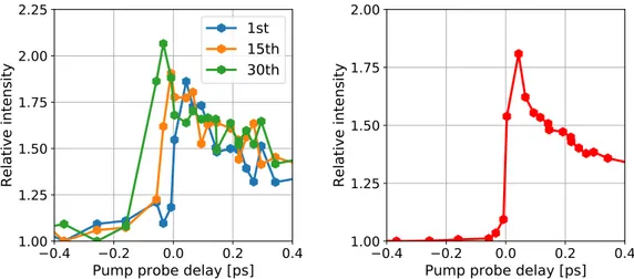
and fast change when the pump pulse hits. The number of electrons detected above the Fermi energy for individual scans of a measurement series on an iron sample are displayed in the left of 1.11. They show a change of time zero by roughly 100 fs. The individual traces are shifted s.t. the positions of the maxima end up at the same pump probe delay. The resulting overall signal, on the right of the figure, displays the same time resolution as the single scans.
The other shift that can occur is one in energy. It is caused by the varying strength of the previously discussed space charge effect due to a change (usually decrease) of the incident UV intensity. There are three common reasons for a reduction in the number of photons arriving at the sample: A drift in the exact optimal setting of the compressor at the end of the laser system leads to longer pulses and hence a lower efficiency of the nonlinear photon conversion processes.
A misalignment of the argon jet and the driving beam strongly suppresses high harmonic generation. Finally, carbon deposition on the UV optics, especially on
Figure 1.11: Traces of the number of electrons detected above the Fermi en- ergy. For several individual scans on the left (scan number in the legend) and integrated over the whole measurement series after correction on the right.
the mirrors, reduces the UV radiation transmitted from source to sample [54, 55].
The energy shift is resolved in a similar way as the one in t0. A clear spectral feature is determined in single scans, usually the Fermi edge, which is then set to the same energy for all scans.
The data for both magnetization directions go through all the steps separately.
Asymmetry and hence spin polarization calculation is always the last step for the following reason: The division by the total number of electrons at a certain energy and angle leads to a relative amplification of data points with low statistics.
Therefore, binning or averaging over asymmetry or polarization lacks appropriate weighting. This is well illustrated by the following extreme example: We average asymmetry over two pixels of the detector. One of them records 500 electrons for both magnetization directions, leading to an asymmetry of 0%. The other one detects only a single electron, along the majority direction, corresponding to 100% asymmetry. For the binned data point this results in a value of 50%, which is far from the actual value of 0.1% for the selected range.
Demagnetization Experiments
This first experimental chapter considers ultrafast demagnetization measure- ments on thin iron films using the STARPES setup. The obtained data re- veals different dynamics for different parts of the emitted spectrum. This is only possible due to the simultaneous availability of resolution in energy and spin polarization. We further investigate the topic by a study on the fluence dependence of spin depolarization at different binding energies. Comparison of MOKE, a widely used technique in the field for magnetization dynamics, with photoemission lead to the conclusion, that this optical technique follows closely the dynamics close to the Fermi energy. Furthermore, we present experimental evidence for a transient spin voltage, i.e. the splitting of the respective chemical potentials.
2.1 Introduction
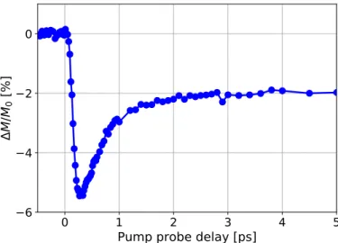
The term ultrafast demagnetization refers to the partial or complete loss of the magnetic order parameterMwithin less than one picosecond or even one hundred femtoseconds after an ultrashort excitation. The ultrafast decrease is followed by a rapid (ps) and a slower (ns) recovery of M as long as the excitation lies under a sample specific threshold. A typical demagnetization trace we have measured on nickel by MOKE shows these three steps as visible in figure 2.1.
Figure 2.1: Trace of ultrafast demagnetization measured on nickel by the mag- neto optical Kerr effect.
The phenomenon has been observed in 3d-transition metals, some alloys con- taining significant fractures of them [56] and also magnetic multilayer structures [57]. Its discovery in Kerr experiments using a pulsed laser source on nickel changed the understanding of the dynamic behavior of magnetism [58]. Be- fore, the spin system was considered only coupled to the lattice via magnetic anisotropy, which is caused by spin orbit coupling (SOC) without a direct con- nection to the electronic degrees of freedom. However, the energy scale corre- sponding to the spin-lattice coupling is on the lower meV range, translating to a time scale clearly above one picosecond [59]. Furthermore, the lattice reaches its
maximal excitation only after roughly one ps [60]. Hence the probability is low that the magnetization follows a signal that is slower than itself.
Ultrafast demagnetization triggered the development of the three tempera- ture model (3TM) [58], an extension of the two temperature model used for the description of electron thermalization in metals [61]. In this model a solid is divided into the three subsystems of electrons (charge), phonons (lattice) and spins (magnetization). An individual temperature is assigned to each of them (Te, Tp and Ts respectively). The three temperatures are coupled by a set of differential equations defined by system specific coupling constants gij and heat capacities Ci. The model is completed when terms for a time dependent source S(t) (representing an exciting laser pulse) and heat diffusion κ∆Te are added to the equation describing the evolution of the electron temperature:
Ce(Te)dTe
dt =S(t) +κ∆Te+gep(Tp−Te) +ges(Ts−Te) (2.1) Cp(Tp)dTp
dt =gep(Te−Tp)−gps(Tp−Ts) (2.2) Cs(Ts)dTs
dt =ges(Te−Ts) +gps(Tp −Ts) (2.3) In turns out that the coupling between phonons and spinsgps is more than an order of magnitude smaller than the other two, that have typically very similar values [58]. Therefore, it is often neglected in later publications [62].
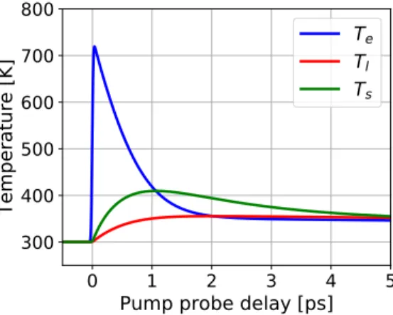
Implementation of this model for the case of nickel and an incidence optical excitation fluence on the order of 1 cmmJ2 produces temperature traces shown in figure 2.2. The ultrafast excitationS(t) induces a very sharp rise ofTe. Since the ratio of coupling constant to heat capacity is larger for the spin than the phonon system, Ts rises steeper and crosses the electronic temperature sooner than Tp. The steep rise of the spin temperature corresponds to the demagnetization pro- cess. The consequent decay, again following Te, until pseudo-equilibration with Tp marks the fast recovery. The cooldown of all three systems together by heat diffusion translates to the slow second part of the recovery.
Despite its simplicity, the phenomenological description provided by the 3TM is a powerful tool for predicting the behavior of a magnetic system upon excitation.
Figure 2.2: Traces of the three separate temperatures of the electron, lattice and spin system (Te,Tl and Ts) calculated with the 3TM.
However, it does not consider the mechanism behind ultrafast demagnetization.
The effect responsible for the loss of spin polarization and the connected transfer of angular momentum, an overall conserved quantity, is not part of the model.
This unanswered question is under debate in the community since the discovery of ultrafast demagnetization more than twenty years ago. A lot of advances have been made in experiment and theory, but the issue has not come to a final conclusion yet [59].
A few potential mechanisms could be eliminated in measurements with varying excitation. Several experiments identified direct interaction of the spin system with the excitation as insignificant for demagnetization: The influence of the pump photon energy can be inferred from the respective reflection, absorption and extinction coefficients [63]. The same has been found for the polarization state of the pump pulse [64]. The case of intense terahertz pulses as excitation is particularly interesting. Other than in optical or infrared (IR) radiation, the terahertz pump can reach magnetic fields of several Teslas [65], strong enough to induce sub-ps magnetization dynamics. However, in the experiments performed by Shalabyet al. coherent precession of the magnetization in the THz magnetic field was observed but could be completely separated from the ultrafast demag- netization, i.e. the strong magnetic filed had no effect on it as shown by doing the same measurement with changed THz polarization [66]. A study on the effect