From Tapering to Tightening

Policy Research Working Paper 7071

From Tapering to Tightening

The Impact of the Fed’s Exit on India

Kaushik Basu Barry Eichengreen

Poonam Gupta

Development Economics Vice Presidency Office of the Chief Economist

October 2014

WPS7071

Public Disclosure Authorized Public Disclosure Authorized Public Disclosure Authorized Public Disclosure Authorized

Produced by the Research Support Team

Abstract

The Policy Research Working Paper Series disseminates the findings of work in progress to encourage the exchange of ideas about development issues. An objective of the series is to get the findings out quickly, even if the presentations are less than fully polished. The papers carry the names of the authors and should be cited accordingly. The findings, interpretations, and conclusions expressed in this paper are entirely those of the authors. They do not necessarily represent the views of the International Bank for Reconstruction and Development/World Bank and its affiliated organizations, or those of the Executive Directors of the World Bank or the governments they represent.

Policy Research Working Paper 7071

This paper is a product of the Office of the Chief Economist, Development Economics Vice Presidency. It is part of a larger effort by the World Bank to provide open access to its research and make a contribution to development policy discussions around the world. Policy Research Working Papers are also posted on the Web at http://econ.worldbank.org. The authors may be contacted at pgupta5@worldbank.org.

The “tapering talk” starting on May 22, 2013, when Federal Reserve Chairman Ben Bernanke first spoke of the possibil- ity of the U.S. central bank reducing its security purchases, had a sharp negative impact on emerging markets. India was among those hardest hit. The rupee depreciated by 18 percent at one point, causing concerns that the country was heading toward a financial crisis. This paper contends that India was adversely impacted because it had received large capital flows in prior years and had large and liquid financial markets that were a convenient target for investors seek- ing to rebalance away from emerging markets. In addition, India’s macroeconomic conditions had weakened in prior years, which rendered the economy vulnerable to capital outflows and limited the policy room for maneuver. The paper finds that the measures adopted to handle the impact

of the tapering talk were not effective in stabilizing the financial markets and restoring confidence, implying that there may not be any easy choices when a country is caught in the midst of rebalancing of global portfolios. The authors suggest putting in place a medium-term policy framework that limits vulnerabilities in advance, while maximizing the policy space for responding to shocks. Elements of such a framework include a sound fiscal balance, sustainable current account deficit, and environment conducive to investment.

In addition, India should continue to encourage relatively

stable longer-term flows and discourage volatile short-term

flows, hold a larger stock of reserves, avoid excessive appre-

ciation of the exchange rate through interventions with the

use of reserves and macroprudential policy, and prepare the

banks and firms to handle greater exchange rate volatility.

From Tapering to Tightening:

The Impact of the Fed’s Exit on India

Kaushik Basu, Barry Eichengreen and Poonam Gupta

Keywords: Balance of Payments, Economic Management, Macroeconomic Policy, Macroeconomic Vulnerability, Monetary Policy

1

We thank Shankar Acharya, Rahul Anand, Paul Cashin, Tito Cordella, Manoj Govil, Muneesh Kapur, Ken Kletzer, Rakesh Mohan, Zia Qureshi, Y.V. Reddy, David Rosenblatt, Aristomene Varoudakis, and

participants of the India Policy Forum, 2014, for very useful discussions and comments, and Serhat Solmaz for excellent research assistance.

I. Introduction

On May 22, 2013, Federal Reserve Chairman Ben Bernanke first spoke of the possibility of the Fed tapering its security purchases. His “tapering talk” had a sharp negative impact on financial conditions in emerging markets.

India was among those hardest hit. Between May 22, 2013, and the end of August 2013, its exchange rate depreciated by 18 percent, bond spreads increased, and equity prices fell. The reaction was sufficiently pronounced for the press to warn that India might be heading toward a full-blown financial crisis, the kind that requires a country to seek IMF assistance.

In this paper we ask three questions about this episode. Why was the impact of the Fed’s announcement on India’s financial markets so severe? How effective were the policy measures undertaken in response? How can India prepare itself for the normalization of monetary policy in advanced economies and more broadly to react to global liquidity cycles?

Eichengreen and Gupta (2014) analyzed the impact of the Fed’s tapering talk on exchange rates, foreign reserves and equity prices in emerging markets between April and August 2013.

They established that an important determinant of the impact was the volume of capital flows that countries received in prior years and the size of their local financial markets. Those which received larger inflows of capital and had larger and liquid financial markets experienced more pressure on their exchange rates, reserves, and equity prices once the “tapering talk” began. This may be interpreted as showing that investors are better able to rebalance their portfolios away from an emerging economy when the country in question has a relatively large and liquid financial market.

This paper elaborates the Indian case. India ranks high in terms of the size and liquidity of its financial markets and the extent of capital flows it received in prior years and became an easy target for investors seeking to rebalance away from emerging markets.

In addition, Eichengreen and Gupta show that the emerging markets that had allowed their real exchange rate to appreciate and the current account deficit to widen during the period of quantitative easing felt a larger impact. Similar vulnerabilities had built in India too in prior years. Its current account deficit had increased and real exchange rate had appreciated markedly. In addition, its fiscal deficit had increased, and inflation at about 10 percent was proving to be stubbornly high.

These macroeconomic weaknesses had surfaced in the midst of a sharp growth slowdown. Although the level of foreign reserves was considered comfortable by some metrics, the effective coverage they provided had declined unmistakably since 2008.

2

The period of the tapering talk is generally referred to that between May 22, 2013 and September 18, 2013.

3

See e.g . “India in crisis mode as rupee hits another record low”,

http://money.cnn.com/2013/08/28/investing/india-rupee/; “India’s Financial Crisis, Through the Keyhole”, http://www.economist.com/blogs/banyan/2013/08/india-s-financial-crisis.

4

Subsequently the Federal Reserve started tapering its purchases of securities in December 2013, reducing it by $10 bn each month. It has since then tapered six more times, each time by $10 bn and is expected to end the program in October, 2014, with a last reduction of $15 bn in the purchase of securities.

2

The specific factors contributing to the high fiscal or current account deficit in India also indicated increased economic and financial vulnerabilities. The increase in fiscal deficit was due to an increase in current expenditure (in response to the global financial crisis of 2008, the headwinds of which were palpable in India by early 2009), rather than to a pick-up in public investment. The increase in current account deficit, largely a mirror effect of the increased current expenditure, was characterized by some deflection of private savings into the import of gold. It reflected a dearth of attractive domestic outlets for personal savings in a high inflation environment, where real returns on many domestic financial investments had turned negative. Loose monetary policy in advanced countries meanwhile made those deficits easy to finance, further relieving the pressure to compress them. Rebalancing by global investors when the Fed broached the subject of tapering highlighted these vulnerabilities.

The authorities adopted a range of measures in response. They intervened in the foreign exchange market, hiked interest rates, raised the import duty on gold, encouraged capital inflows from nonresident Indians, eased demand pressure in the foreign exchange market by opening a separate swap window for oil importing companies, opened a swap line with the Bank of Japan, and restricted capital outflows from residents and Indian companies. We empirically estimate the impact of these measures on the exchange rate and financial markets. Our results show that some of these measures, including the separate swap window for oil importing companies, were of limited help in stabilizing the financial markets. Others, like initiatives restricting capital outflows, actually

undermined confidence and proved counterproductive.

The results imply that there may not be any easy choices when a country is in the midst of rebalancing of global portfolios. We suggest putting in place a medium-term policy framework that limits vulnerabilities in advance, while maximizing the policy space for responding to shocks.

Elements of such a framework include holding a larger stock of reserves; avoiding excessive appreciation of the exchange rate through interventions using reserves and macroprudential policy;

signing swap lines with other central banks where feasible; preparing the banks and the corporates to handle greater exchange rate volatility; adopting a clear communication strategy; avoiding measures that could damage confidence, such as restricting outflows; and managing capital inflows to

encourage relatively stable longer-term flows while discouraging short-term flows.

A sound fiscal balance, sustainable current account deficit, and environment conducive for investment are other more obvious elements of this policy framework.

5

See Zhang and Zoli (2014) and the literature cited therein for the recent contributions on the use of macro

prudential policies, in particular loan to value ratio, debt to income ratio, required reserves ratio,

countercyclical provisioning and countercyclical capital requirements in Asian economies. See Cordella, Vegh and Vuletin (2014) on the use of reserve requirements as a countercyclical macroprudential tool in developing countries.

3

II. The Effects of the Tapering Talk on India

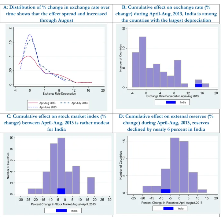
As documented in Eichengreen and Gupta (2013), the tapering talk affected a large number of emerging markets. Using the data for 53 emerging markets (which have their own currency and exchange rate), they calculated cumulative changes in their exchange rates, stock prices, bond spreads and reserves between April 2013 and, alternatively, end of June, end of July and end of August 2013. The resulting distribution of exchange rate changes over the months through August is portrayed in Panel A of Figure 1. The data show that the exchange rate depreciated in 36 of the 53 countries between April and June.

Despite some subsequent recovery, by August exchange rates for 30 of the 53 countries remained below their levels seen in April. The average rate of depreciation in these 30 countries was over 6 percent, and exchange rates for about half the countries depreciated by more than 5½ percent.

Panel B provides further details on the distribution of exchange rate changes between April and August. The largest depreciation was experienced by Brazil, India, South Africa, Turkey and Uruguay, where the exchange rate depreciated by at least 9 percent, and Brazil experienced the largest depreciation of 17 percent. Data for stock markets are available for fewer countries; 25 of the 38 countries for which we have the data experienced some decline in their stock markets. The average decline in these 25 countries was 6.9 percent (Panel C, Figure 1). For six emerging markets (Chile, Indonesia, Kazakhstan, Peru, Serbia, and Turkey), the decline was more than 10 percent. In comparison, India had a relatively modest decline in its stock market (at month-end values).

Reserves declined for 29 of 51 countries between April and August, with the largest declines seen in the Dominican Republic, Hungary, Indonesia, Sri Lanka, and Ukraine.

6

We extracted the data on exchange rate, reserves and stock markets from the Global Economic Monitoring database of the World Bank, on October 29, 2013.

7

We dropped countries where events other than the tapering talk clearly dominated the impact on financial markets. For example Pakistan where there was a large increase in stock prices due to developments unrelated to tapering—it had agreed to a $5.3 billion loan from the IMF on July 5, boosting reserves and leading to rallies in stocks, bonds and the rupee (Bloomberg, July 5, 2013). We also dropped Egypt where foreign reserves rose by 33 percent between April and July, 2013 due to aid from other countries.

4

Figure 1: Exchange Rate, Stock Market and Reserves in Emerging Markets during the Tapering Talk

A: Distribution of % change in exchange rate over time shows that the effect spread and increased

through August

B: Cumulative effect on exchange rate (%

change) during April-Aug, 2013, India is among the countries with the largest depreciation

C: Cumulative effect on stock market index (%

change) between April-Aug, 2013 is rather modest for India

D: Cumulative effect on external reserves (%

change) during April-Aug, 2013, reserves declined by nearly 6 percent in India

Source: Data on exchange rates, reserves and stock markets are from the Global Economic Monitoring database of the World Bank. Calculations are based on end of month values. See Eichengreen and Gupta (2014) for details.

Even though the tapering talk affected a large number of emerging markets, much of the market commentary focused on five countries, Brazil, Indonesia, India, Turkey and South Africa, christened as “Fragile Five”. Table 1 summarizes the effect on these five countries. As is evident from the table, the exchange rates depreciated and reserves declined in all five countries, while equity

0.05.1.15.2

-4 0 4 8 12 16 20

Exchange Rate Depreciation Apr-Aug 2013 Apr-July 2013 Apr-June 2013

051015Number of Countries

-4 0 4 8 12 16 20

Exchange Rate Depreciation April-Aug 2013 India

0246810Number of Countries

-30 -25 -20 -15 -10 -5 0 5 10 15 20 25 30 Percent Change in Stock Market August-April, 2013

India

051015Number of Countries

-25 -20 -15 -10 -5 0 5 10 15 20

Percent Change in Reserves April-August,2013 India

5

prices declined in all but South Africa. The largest exchange rate depreciation occurred in Brazil, the largest decline in stock prices was in Turkey, and the largest reserve loss was observed in Indonesia.

Within this group India had the second largest exchange rate depreciation and the second largest decline in reserves.

Table 1: Effect of Tapering Talk on “Fragile Five” Countries (April-August, 2013)

Exchange Rate

Depreciation % change in Stock

Prices % Change in

Reserves

Brazil 17.01 -5.28 -3.07

Indonesia 8.33 -14.21 -13.30

India 15.70 -3.32* -5.89

Turkey 9.21 -15.38 -4.56

South Africa 10.60 6.81 -5.05

Note: Calculated using data from the Global Economic Monitor database of the World Bank. * Decline in stock prices in India was about 10 percent if calculated using daily data between May 22 and August 31, 2013.

This period was also marked by significant volatility in financial markets in the affected countries. Highlighting the Indian case in Table 2, we show that the short-term volatility, measured by the standard deviation of percentage change in exchange rates, stock market prices and reserves (using daily data for exchange rate and equity prices and weekly data for reserves) was quite large in summer 2013, compared to the previous months.

Table 2: Volatility in India during the Tapering Talk (Standard deviation of percent changes using daily or weekly data)

s.d. of % change in

daily exchange rate

s.d. of % change in

daily stock prices s.d. of % change in weekly stock of foreign reserves Tapering Talk: May 23, 2013-

August 31, 2013 4.95 3.62 1.82

Previous three Months (Feb 21,

2013-May 22, 2013) 0.9 2.81 0.73

Previous one year (May 21, 2012-

May 22, 2013) 1.71 6.92 1.05

Note: Standard deviation calculated using daily data on nominal exchange rate and stock market index from Bloomberg; and weekly data on foreign reserves from the RBI.

6

III. Why Was India Affected So Severely?

We contend that the impact was large on India for two reasons. First, India’s large and liquid financial markets had received significant volumes of capital flows in prior years, making it a

convenient target for investors seeking to rebalance away from emerging markets; and second, its macroeconomic vulnerabilities had increased in the years prior to the tapering talk, making it vulnerable to capital outflows and limiting the policy room to address the shock that the tapering talk initiated.

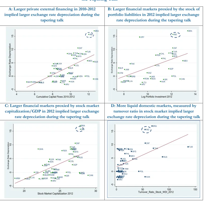
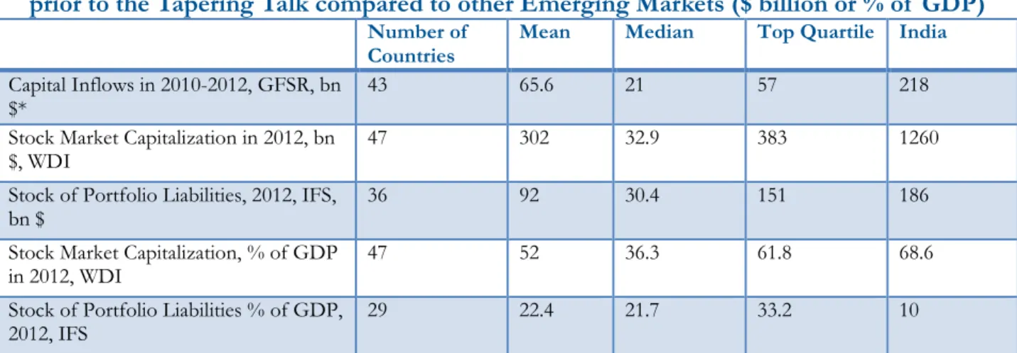
In their analysis of the impact of the Fed’s tapering talk on the exchange rates, foreign reserves and equity prices of emerging markets between May 2013 and August 2013, Eichengreen and Gupta (2014) found that the countries with larger financial markets and larger capital inflows in the prior years experienced more exchange rate depreciation and larger reserve losses during the tapering talk. Evidently, investors are more easily able to rebalance their portfolios away from an economy when the country in question has a relatively large and liquid financial market (possibly they incur a smaller loss of value and need to withdraw only from a few large markets than sell their assets in many small markets). India ranks high in terms of the size and liquidity of its financial markets and the extent of capital flows it received in prior years (see Figure 2 and Table 3). Whether measured in absolute terms or as percent of GDP, India is among the top quartile of countries, or for some indicators among the top few emerging economies, for various measures of the size and liquidity of financial markets.

7

Figure 2: Size and Liquidity of Financial Markets and the Effect on Exchange Rate during the Tapering Talk

A: Larger private external financing in 2010-2012 implied larger exchange rate depreciation during the

tapering talk

B: Larger financial markets proxied by the stock of portfolio liabilities in 2012 implied larger exchange

rate depreciation during the tapering talk

C: Larger financial markets proxied by stock market capitalization/GDP in 2012 implied larger exchange

rate depreciation during the tapering talk

D: More liquid domestic markets, measured by turnover ratio in stock market implied larger exchange rate depreciation during the tapering talk

Source: Eichengreen and Gupta (2014)

ARM ALB

AZE BGR BIH

BLR

BRA

CHL

CHN COL

CRI DOM

GHA

GTM

HRVHUN IDN

IND

JAM JOR

KAZ KEN

LBN LKA

LVA LTUMAR

MEX

MKD

MYS PAK

PER PHL

ROM POL

RUS

SRB

THA

TUN

TUR

UKR VEN VNM

ZAF

-5051015Exchange Rate Depreciation

4 6 8 10 12

Cumulative Capital Flows 2010-2012

BGR BLR

BRA

CHL

CHN COL

GTM

HRV HUN

IDN IND

ISR JAM

JOR

KAZ LVA LTU

MAR

MEX

MUS

MYS PAK

PER PHL

ROM POL

SGP SRB

THATUR

UKR URY

ZAF

-5051015Exchange Rate Depreciation

8 10 12 14

Log Portfolio Investment 2012

ARM BGR

BRA

CHL

CHN COL

CRI

CZE GHA

HKG HRV

HUN

IDN IND

ISR JAM

JOR KAZ KEN

LBN KOR LKA

LVA LTU MAR

MEX

MKD

MUS

MYS PAK

PER PHL

ROM POL

RUS SGP SRB

THA

TUN

TUR

UKRVENVNM

ZAF

-5051015Exchange Rate Depreciation

20 25 30

Stock Market Capitalization 2012

ARG

ARMBGR

BRA

CHL

COL

CRI GHA

HRV HUN

IDN

IND

JAM JOR KAZ

KEN LBN

LKA

LVALTUMAR MEX

MYS PAK PER

PHL

ROU POL

RUS

SRB

THA

TUN

TUR

VENUKRVNM

ZAF

-5051015

0 50 100 150

Turnover_Ratio_Stock_WDI_2012

8

Table 3: Size of the Financial Market and Cumulative Capital Inflows were Large in India prior to the Tapering Talk compared to other Emerging Markets ($ billion or % of GDP)

Number of

Countries Mean Median Top Quartile India

Capital Inflows in 2010-2012, GFSR, bn

$* 43 65.6 21 57 218

Stock Market Capitalization in 2012, bn

$, WDI 47 302 32.9 383 1260

Stock of Portfolio Liabilities, 2012, IFS,

bn $ 36 92 30.4 151 186

Stock Market Capitalization, % of GDP

in 2012, WDI 47 52 36.3 61.8 68.6

Stock of Portfolio Liabilities % of GDP,

2012, IFS 29 22.4 21.7 33.2 10

Note: Data on capital inflows, consisting of private inflows of bonds, equity, and loans is from the IMF’s Global Financial Stability Report. Data on stock market capitalization is from the World Development Indicators; and the data on portfolio liability is from the International Financial Statistics.

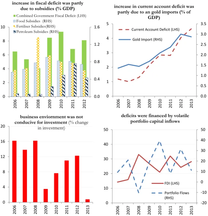
A second reason for the impact of the Fed’s tapering talk on India was the macroeconomic imbalances that were apparent at its outset. Eichengreen and Gupta show that the emerging markets that had allowed their real exchange rate to appreciate and the current account deficit to widen during the period of quantitative easing saw a larger impact. Similar vulnerabilities had built in India too in prior years. Its current account deficit had increased from about 1 percent of GDP in 2006 to nearly 5 percent in 2013; and its real exchange rate had appreciated markedly. In addition, the fiscal deficit had increased, and inflation at about 10 percent was proving to be stubbornly high (Figure 3).

These macroeconomic weaknesses had surfaced in the midst of a sharp growth slowdown. Although the level of foreign reserves was considered comfortable by some metrics, the effective coverage they provided had declined unmistakably since 2008. The policy interest rate was high, having been increased by the Reserve Bank of India (RBI) from 3.25 percent in December 2009 to 8.50 percent in December 2012. The large fiscal deficit and high policy rate implied little room for maneuver in fiscal and monetary policy.

Specific factors contributing to the high fiscal or current account deficit also indicated increased economic and financial vulnerabilities. The increase in fiscal deficit was due to an increase in current expenditure, in response to the global financial crisis of 2008, the headwinds of which were palpable in India by early 2009, rather than to a pick-up in public investment. The increase in current account deficit, largely a mirror effect of the increased current expenditure, was

characterized by some deflection of private savings into the import of gold, reflecting a dearth of attractive domestic outlets for personal savings in a high inflation environment, where real returns on many domestic financial investments had turned negative (see Figure 4). Loose monetary policy in advanced countries meanwhile made those deficits easy to finance, further relieving the pressure to compress them.

8

In a paper presented at India Policy Forum, 2013, Kapur and Mohan had cautioned that such macroeconomic imbalances indicated heightened vulnerabilities to a financial crisis.

9

Figure 3: Macroeconomic Imbalances were apparent in India at the outset of the Tapering Talk

Growth Rate was declining… Inflation was Persistently High….

Fiscal deficit was High… Current Account Deficit was Increasing…

Reserve Coverage had Declined Real Exchange Rate had Appreciated

Sources: GDP, CSO; CPI Inflation, Citi Research; Gross Fiscal Deficit, Current Account Deficit, Reserve Bank of India;

Reserves to M2 Ratio, IFS; Real Effective Exchange Rate (CPI based, six currency), RBI; Bilateral RER calculated using data from IFS. Years refer to fiscal years.

3 4 5 6 7 8 9 10

2006 2007 2008 2009 2010 2011 2012 2013

GDP Growth

3 5 7 9 11 13

2006 2007 2008 2009 2010 2011 2012 2013

CPI Inflation

3 4 5 6 7 8 9 10

2006 2007 2008 2009 2010 2011 2012 2013

Combined Fiscal Deficit, % of GDP

0 1 2 3 4 5

2006 2007 2008 2009 2010 2011 2012 2013

Current Account Deficit, % of GDP

20 25 30 35

2006 2007 2008 2009 2010 2011 2012 2013

India Reserves to M2 Ratio

95 105 115 125 135

2006 2007 2008 2009 2010 2011 2012 2013

Real Exchange Rate (2006=100)

Real Effective Exchange Bilateral RER with USD

10

Figure 4: The Level and Quality of Fiscal Deficit and Current Account Deficit indicated Vulnerabilities at the outset of the Tapering Talk

Sources: Gross Fiscal Deficit, FDI, Gold Import, Current Account Deficit, Reserve Bank of India; Subsidies, Ministry of Petroleum and Natural Gas, Govt. of India; Investment, CSO; Portfolio Flows, Bloomberg.

0.0 0.4 0.8 1.2 1.6

0 2 4 6 8 10

2006 2007 2008 2009 2010 2011 2012

increase in fiscal deficit was partly due to subsidies (% GDP)

Combined Government Fiscal Deficit (LHS) Food Subsidies (RHS)

Fertiliser Subsidies(RHS) Petroleum Subsidies (RHS)

0.0 0.5 1.0 1.5 2.0 2.5 3.0 3.5

0 1 2 3 4 5

2006 2007 2008 2009 2010 2011 2012 2013

increase in current account deficit was partly due to an gold imports (% of

GDP)

Current Account Deficit (LHS) Gold Import (RHS)

0 4 8 12 16 20

2006 2007 2008 2009 2010 2011 2012 2013

business enviornment was not conducive for investment (% change

in investment)

-20 -10 0 10 20 30 40 50

0 10 20 30 40 50

2006 2007 2008 2009 2010 2011 2012 2013

deficits were financed by volatile portfolio capital inflows

FDI (LHS) Portfolio Flows (RHS)

11

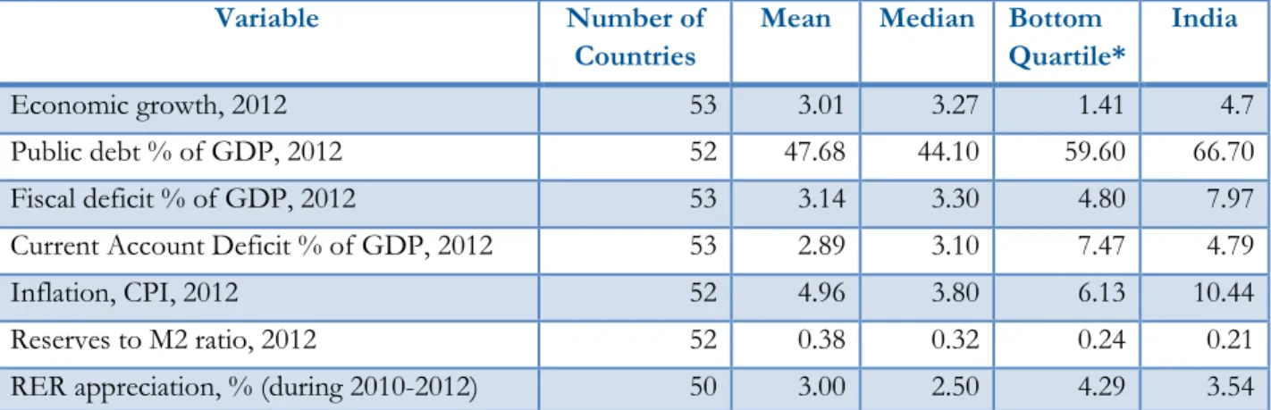
India fared worse than the median emerging market for most of the indicators of the macroeconomic vulnerabilities, or worse than the three-fourths of them for some of the indicators, including the level of debt, fiscal deficit, inflation and reserves (Table 4).

Table 4: Comparison of Macroeconomic Variables for India with other Emerging Markets in 2012

Variable Number of

Countries Mean Median Bottom

Quartile* India

Economic growth, 2012 53 3.01 3.27 1.41 4.7

Public debt % of GDP, 2012 52 47.68 44.10 59.60 66.70

Fiscal deficit % of GDP, 2012 53 3.14 3.30 4.80 7.97

Current Account Deficit % of GDP, 2012 53 2.89 3.10 7.47 4.79

Inflation, CPI, 2012 52 4.96 3.80 6.13 10.44

Reserves to M2 ratio, 2012 52 0.38 0.32 0.24 0.21

RER appreciation, % (during 2010-2012) 50 3.00 2.50 4.29 3.54

Note: *values refer to the country at the bottom 25 percentile for economic growth and reserves and the country at the top 25 percentile for all other variables. Sources as in Eichengreen and Gupta (2014).

Drawing on Eichengreen and Gupta (2014), we consider the factors that were associated with the impact of the tapering talk on exchange rate as well as on stock prices and reserves. We calculate weighted average of changes in exchange rates, foreign reserves and stock prices in two separate indices. We calculate the first index, which we call the Capital Market Pressure Index I, as a weighted average of percent depreciation of exchange rate and reserves losses between April 2013 and August 2013, where the weights are the inverse of the standard deviations of monthly data from January 2000 to August 2013.

Capital Market Pressure Index I = % 𝐸𝑥𝑐ℎ𝑎𝑛𝑔𝑒 𝑅𝑎𝑡𝑒 𝐷𝑒𝑝𝑟𝑒𝑐𝑖𝑎𝑡𝑖𝑜𝑛

𝜎

+ % 𝐷𝑒𝑐𝑙𝑖𝑛𝑒 𝑖𝑛 𝑅𝑒𝑠𝑒𝑟𝑣𝑒𝑠 𝜎

A second index, Capital Market Pressure Index II, is similarly constructed as a weighted average of the percent depreciation of exchange rate, reserve loss and decline in stock prices between April 2013 and August 2013.

9

We construct these indices in a manner analogous to the exchange market pressure index in Eichengreen, Rose and Wyplosz (1995), which they constructed as a weighted average of changes in exchange rates, reserves, and policy interest rates, where the weights are the inverse of the standard deviation of each series.

The number of countries for which we can construct the index declines from 51 for the first index to 37 for the second index. If we also include increase in bond yields in the index, the number of countries for which we would be able to construct it declines to 25.

12

Capital Market Pressure Index II

= % 𝐸𝑥𝑐ℎ𝑎𝑛𝑔𝑒 𝑅𝑎𝑡𝑒 𝐷𝑒𝑝𝑟𝑒𝑐𝑖𝑎𝑡𝑖𝑜𝑛

𝜎

+ % 𝐷𝑒𝑐𝑙𝑖𝑛𝑒 𝑖𝑛 𝑅𝑒𝑠𝑒𝑟𝑣𝑒𝑠 𝜎

+ % 𝐷𝑒𝑐𝑙𝑖𝑛𝑒 𝑖𝑛 𝑆𝑡𝑜𝑐𝑘 𝑀𝑎𝑟𝑘𝑒𝑡 𝜎

We regress exchange rate depreciation, Index I and Index II on macroeconomic conditions, financial market structure and institutional variables, estimating linear equations of the form:

Y

= α

X

+ε

(1)

where Y

is exchange rate depreciation, Index I or Index II for country i between April-August 2013.

The explanatory variables, X

, include cumulative private capital inflows during 2010-2012, stock of portfolio liabilities or stock market capitalization in 2012 as alternate measures of the size of

financial markets; several alternate measures of macroeconomic conditions such as the increase in current account deficit, real exchange rate appreciation, foreign reserves, GDP growth, fiscal deficit, inflation or public debt; and institutional variables such as the exchange rate regime, capital account openness, or the quality of the business environment.

Since these variables are correlated, we include only one of them at a time from each

category (size of financial markets, macroeconomic variables, and institutional variables). Results are similar using different proxies, reassuringly, so we report only a representative subset here. We take the values of the regressors in 2012 or their averages over the period 2010–2012 (either way, prior to the tapering talk).

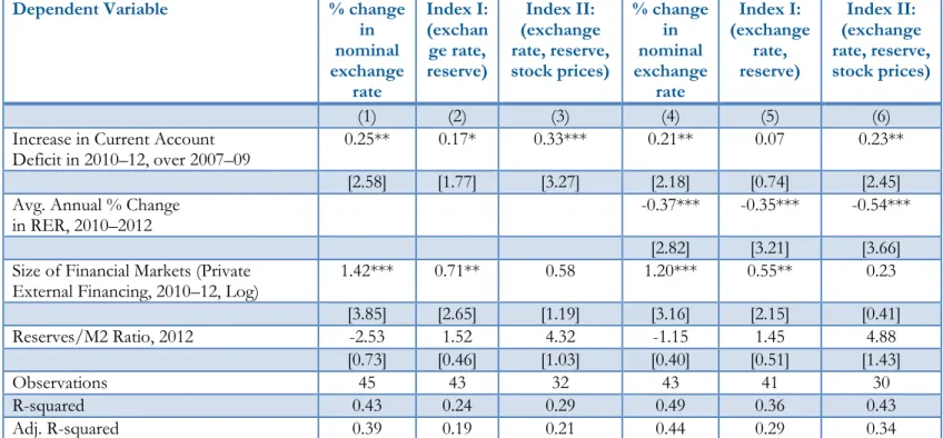
Results show that the countries with larger financial markets experienced larger exchange rate depreciation and reserve losses. Also evidently, deterioration in current account, extent of real exchange rate appreciation, and inflation (results are not reported here for specifications in which we include inflation, but are available on request) during the years of abundant global liquidity were associated with more exchange rate depreciation and larger increases in the composite indices in the summer of 2013 (Table 5).

This helps us understand why the same countries that complained about the impact of quantitative easing on their exchange rates in the earlier years also complained about the impact of the tapering talk in the summer of 2013. The countries most affected by or least able to limit the earlier impact on their real exchange rates were the same ones to subsequently experience large and uncomfortable real exchange rate reversals, in other words. Standardized coefficients, to compare

10

We also consider some other available measures of the size and liquidity of the financial markets. The alternate measures are strongly correlated with each other and give similar results. Results hold if we calculate the dependent variables for April-July, 2013. Since most of these variables are persistent and correlated across years, it turns out to be inconsequential whether we use the data for just one year or period averages. More detailed results are available in Eichengreen and Gupta (2014).

13

quantitatively the coefficients of various regressors, show that the coefficient of the size of financial markets is the largest followed by the coefficients of real exchange rate and current account deficit.

We do not find any other macroeconomic or institutional variables to be associated significantly with the impact of the tapering talk on the exchange rate or other variables.

Table 5: Regression Results for Factors Associated with Exchange Rate Depreciation and Capital Market Pressure Indices during April-August 2013

Dependent Variable % change

nominal in exchange

rate

Index I:

(exchan ge rate, reserve)

Index II:

(exchange rate, reserve, stock prices)

% change nominal in exchange

rate

Index I:

(exchange rate, reserve)

Index II:

(exchange rate, reserve, stock prices)

(1) (2) (3) (4) (5) (6)

Increase in Current Account

Deficit in 2010–12, over 2007–09 0.25** 0.17* 0.33*** 0.21** 0.07 0.23**

[2.58] [1.77] [3.27] [2.18] [0.74] [2.45]

Avg. Annual % Change

in RER, 2010–2012 -0.37*** -0.35*** -0.54***

[2.82] [3.21] [3.66]

Size of Financial Markets (Private

External Financing, 2010–12, Log) 1.42*** 0.71** 0.58 1.20*** 0.55** 0.23

[3.85] [2.65] [1.19] [3.16] [2.15] [0.41]

Reserves/M2 Ratio, 2012 -2.53 1.52 4.32 -1.15 1.45 4.88

[0.73] [0.46] [1.03] [0.40] [0.51] [1.43]

Observations 45 43 32 43 41 30

R-squared 0.43 0.24 0.29 0.49 0.36 0.43

Adj. R-squared 0.39 0.19 0.21 0.44 0.29 0.34

Note: We calculate average annual percent change in real exchange rate (RER) during 2010-2012, an increase in RER is depreciation;. Current account deficit is calculated as percent of GDP, we take average annual increase in current account deficit during 2010–12 over 2007–09. Index I is constructed as a weighted average of exchange rate depreciation and reserve loss, and Index II as the weighted average of exchange rate

depreciation, reserve loss and decline in the index for stock prices; weights are the inverses of the standard deviations of respective series calculated using monthly data from January 2000 to August 2013. Robust t statistics are in parentheses. *** indicates the coefficients are significant at 1 percent level, ** indicates significance at 5 percent, and * significance at 10 percent level.

IV. Policy Response

India announced a range of policies to contain the impact of the global rebalancing on its exchange rate and financial markets. Most emerging markets increased their policy interest rates and intervened in the foreign exchange market to limit the volatility of the exchange rate and prevent exchange rate overshooting. The RBI similarly intervened in the foreign exchange market to limit the volatility and depreciation of the rupee, spending some $13 billion of reserves between end-May and end-September. Intervention was especially concentrated between June 17 and July 7, when weekly

14

declines in reserves were of the order of $3 billion. The RBI increased its overnight lending rate (the marginal standing facility rate) by 200 basis points to 10.25 percent on July 15

and tightened liquidity through open market operations and by requiring the banks to adhere to reserve requirements more strictly.

Gold imports being partly responsible for a large current account deficit, the government raised the import duty on gold on June 5

, August 13

, and September 18

, increasing it from 6 percent to 15 percent cumulatively. The RBI also imposed controversial new measures on August 14

to restrict capital outflows. These included reducing the limit on the amounts residents could invest abroad or repatriate for various reasons, including for purchasing property abroad.

India being an oil importing country, demand for foreign exchange from companies that import oil can add a significant amount to the overall demand for foreign exchange and thus affect the level and volatility of the exchange rate. The RBI opened a separate swap window for three public sector oil marketing companies on August 28, 2013, to exclude their demand from the foreign exchange market and reduce its volatility.

There were then few additional policy actions in the second half of August, when the exchange rate depreciated most rapidly. This was a period of transition at the RBI, during which governor Dr. Subbarao was to retire on September 4, 2013, and a new governor had to be inducted.

On August 6, 2013, the government announced that on September 4 Raghuram Rajan would take charge as the new governor of the RBI, and in the interim he would join the RBI as an Officer on Special Duty. Little policy communication or guidance was provided by the RBI during this interregnum, over which the exchange rate depreciated by nearly 10 percent.

On September 4, 2013, after formally joining the RBI as the governor, Rajan issued a statement and held a press conference expressing confidence in the economy and highlighting its comfortable reserve position. He announced new measures to attract capital through deposits targeted at nonresident Indians and partially relaxed the restrictions on outward investment introduced previously. Another measure that possibly helped boost the availability of foreign exchange and calm the financial markets around this time was the extension of an existing swap line with Japan, which was increased from $15 billion to $50 billion. The extension of the swap line was negotiated between the Government of India and the Government of Japan and signed by their respective central banks.

We analyze the impact of these policy announcements on financial markets using “event- study” regressions. We compare the values of the exchange rate and financial market variables in a

11

None of these policy measures were novel in the Indian context, having been implemented at different instances in the past, e.g. the import duties on gold were prevalent until the early 1990s; deposits from the Indian diaspora were attracted in a similar fashion twice in the past, in 1998 and in 2000; a separate swap window was made available to the oil importing companies in 2008 to reduce the volatility in the foreign exchange market after the collapse of the Lehman brothers.

15

short window after the policy announcement (we report results for a 5 day post announcement window, but also considered shorter windows of 2 or 3 days which yielded similar results) with those prior to the announcement. For the control period, we consider two options, first, the entire

tapering period from May 22 until the day of the policy announcement, and second, a shorter control period of 1 week prior to the announcement. Below we report results from the specifications in which we use this shorter control period of a week.

The regression specification is given in Equation 2, in which Y is either log exchange rate, log stock market index, portfolio debt flows, or portfolio equity flows (portfolio flows are in millions of US$) ^. For some policy announcements, we also look at the impact on the turnover in the foreign exchange market.

Y

= constant + µ Bond Yield in the US

+ α Tapering Talk Dummy

+ β Dummy for a week prior to Policy Announcement

+ γ Dummy for Policy Announcement

+ ε

(2)

The regressors include US bond yields to account for global liquidity conditions and three

separate dummies, one each for the tapering period (from May 23, 2013-until a week before the policy announcement was made), for the week prior to the policy announcement, and for the week since the policy announcement. We estimate these regressions using data from January 1, 2013, up to the date the policy dummy takes a value of 1, dropping subsequent observations.

(i) Increase in the Interest Rate (July 15)

To assess the impact of increase in interest rates on July 15, we construct the tapering dummy to take a value of 1 from May 23 to July 7, the dummy for the week prior to the

announcement takes a value of 1 from July 8 to July 14, and the dummy for increase in the interest rate takes a value 1 for five consecutive days from July 15 on which the financial markets were open.

The results in Table 6 show that the rate of currency depreciation, equity prices and debt flows did not change significantly following the increase in interest rates. It would appear, then, that this initial policy response was ineffectual.

12

We acknowledge the limitations in being able to establish causality using these regressions, due to the

difficulty in establishing the counterfactual and in controlling for all the relevant factors that may affect the financial markets.

16

Table 6: Effect of the Increase in the Marginal Standing Facility Rate

Note: Data used in the regressions runs from January 1, 2013-July 22, 2013. *, **, *** indicates that the coefficient is significantly different from zero at 10, 5 and 1 percent level of significance, t statistics are in parentheses. # the null hypothesis in each regression is that the policy announcement did not stabilize the market, and the alternative hypothesis is that it stabilized it; 1 percent level of significance is used to test the hypotheses, unless otherwise indicated.

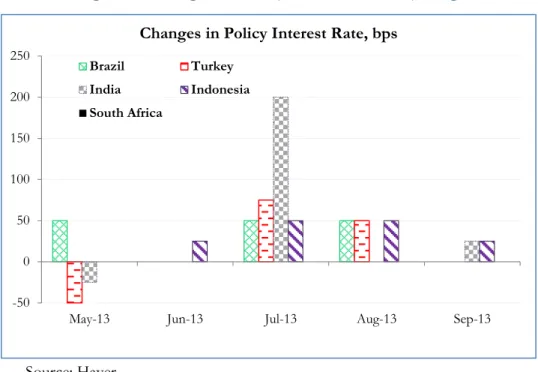
The question is why. Comparing the increase in interest rates in the other Fragile Five countries (Figure 5), we can see that, except for South Africa, the other countries increased interest rates as well. Brazil started raising rates in May and continued doing so through the end of the year;

the increase between May and September totaled 150 basis points. Indonesia first raised rates in July but continued raising them through September; the increase during May-September summed up to 100 basis points. India was different from the other countries in that it raised the interest rate by a larger amount all in one go.

Decisiveness might be thought to signal commitment (this,

presumably, is what the Indian authorities had in mind). Alternatively, a large increase in rates all at once may be perceived as a sign of panic, especially if taken against the backdrop of weak

13

One question of interest is whether a large one time increase is more effective, perhaps for signaling reasons, than several small increases spaced out over months.

(1) (2) (4) (5)

Log Exchange

Rate Log Stock Market

Index Portfolio Debt,

$mn Portfolio Equity,

$mn

US Bond Yield 0.06*** -0.00 -183.96* 9.27

[7.55] [0.25] [1.74] [0.08]

Dummy for tapering

May 22-July 7 (α) 0.04*** -0.01 -233.09*** -189.89***

[9.46] [0.56] [4.32] [3.20]

Dummy for a week prior to July 15, i.e.

from July 8-July 14 (β) 0.05*** 0.00 -4.91 -376.24***

[5.99] [0.15] [0.05] [3.19]

Dummy for a week from July 15 (dummy=1 for 5 working days from July

15) (γ) 0.05*** 0.02 -21.38 -167.71

[6.28] [1.34] [0.21] [1.52]

Results for hypothesis

comparing γ and β

accept Ho: γ

β,

reject Ha: γ

β accept Ho: γ ≤ β,

reject Ha: γ > β accept Ho: γ ≤ β,

reject Ha: γ > β accept Ho: γ ≤ β, reject Ha: γ > β

Constant 3.87*** 8.69*** 399.78** 137.50

[240.80] [264.27] [2.00] [0.63]

Observations 135 138 133 133

R-squared 0.89 0.03 0.40 0.25

Adj. R-squared 0.88 0.004 0.39 0.23

17

fundamentals. Eichengreen and Rose (2003) suggest that sharp increases in rates designed to defend a specific level of asset prices (a specific exchange rate, for example) may be counterproductive when nothing is done at the same time to address underlying weaknesses.

Figure 5: Changes in Policy Interest Rates by Fragile Five

Source: Haver.

(ii) Foreign Exchange Market Intervention

The decline in reserves amounted to some $13 billion between the end of May and end of September, i.e. about 5 percent of the initial stock. Intervention was relatively large from June 17 to July 7, when reserves fell by $3 billion a week. Comparing the extent of intervention in the Fragile Five countries, we see that India and Indonesia intervened the most, and that their intervention was concentrated in June and July.

Not knowing the exact timing of this intervention, we are unable to run event-study

regressions. Moreover, since the pressure to intervene was larger when there was larger depreciation of the currency, one is likely to see a positive correlation between decline in reserves and exchange rate depreciation.

-50 0 50 100 150 200 250

May-13 Jun-13 Jul-13 Aug-13 Sep-13

Changes in Policy Interest Rate, bps

Brazil Turkey

India Indonesia

South Africa

18

Figure 6: Weekly decline in Reserves (billion $) and percent change in Nominal Exchange Rate in India during May 23-End September, 2013

A: Contemporaneous Correlation

B: Reserve Declines lagged by a Week

May-23 May 31

June 7 June 14

June 21

June 28 July 5

July 12

July 19 July 26

Aug 2

Aug 8

Aug 16

Aug 23

Aug 30

Sep 6

Sep 13 Sep 20

Sep 27

-4-2024

-2 -1 0 1 2 3

Decline in Reserves, $ bn

% Depreciation in Nominal Exchange Rate Fitted values

May 31

June 7 June 14

June 21

June 28 July 5

July 12 July 19 July 26

Aug 2

Aug 8 Aug 16

Aug 23

Aug 30

Sep 6

Sep 13 Sep 20

Sep 27

-4-2024

-2 -1 0 1 2 3

Decline in Reserves lagged, $ bn

% Depreciation in Nominal Exchange Rate Fitted values

Exchange Dep=0.28+0.59***Reserve Decline (3.05)

Exchange Dep=0.83-0.26 Reserve Decline, lag (1.06)

19

Figure 6, where we plot the weekly change in reserves and the percentage change in the nominal exchange rate, confirms this. As predicted, we observe a positive correlation in Panel A (significant at the 1 percent level), i.e. a large decline in reserves was associated with greater exchange rate depreciation. In Panel B, we correlate percentage changes in the exchange rate and reserves, where the latter is lagged by a week. Here the correlation between the lagged values of decline in reserves and exchange rate depreciation is indistinguishable from zero.

For one specific intervention announcement, however, we can do better. This is the foreign exchange swap window provided for oil importers. Oil adds up to $10 billion a month to India’s import bill. The demand for foreign exchange thus affects the level and volatility of the exchange rate (as per some estimates, the demand for foreign exchange from these companies is about $400 million a day). With this in mind, the RBI opened a separate swap window for three public sector oil companies on August 28, 2013, so as to remove their demand from the foreign exchange market.

The measure can be thought of as analogous to foreign exchange market intervention, where rather than intervening when the demand for foreign exchange in general increases, the RBI automatically intervenes to meet the demand from the oil companies.

But why this particular form of foreign exchange market intervention should be preferable is not entirely clear. Moreover, it is not obvious either, whether with a daily turnover of about $50 billion in the onshore foreign exchange market, and presumably an equally large offshore market, the amount made available through the special swap window translated into a significant reduction in the demand for foreign exchange.

While some commentators reacted positively to this announcement, we find little evidence of a favorable impact on turnover in the onshore foreign exchange market, the exchange rate or equity markets in the week following. If anything, exchange rate depreciation accelerated in the week after this policy was announced (Table 7).

14

Similar charts for Turkey and Brazil, two other countries for which we have the weekly data on reserves, showed a similar relationship between the decline in reserves and exchange rate depreciation.

20

Table 7: Effect of the Separate Swap Window for Oil Importing Companies on Financial Markets

Note: Data used in the regressions runs from January 1, 2013-July 22, 2013. *, **, *** indicates that the coefficient is significantly different from zero at 10, 5 and 1 percent level of significance, t statistics are in parentheses. # the null hypothesis in each regression is that the policy announcement did not succeed in stabilizing the market, and the alternative hypothesis is that it succeeded; 1 percent level of significance is used to test the hypotheses, unless otherwise indicated.

(iii) Restrictions on Capital Outflows

On August 14, 2013, the RBI announced restrictions on capital outflows from Indian corporates and individuals. It lowered the limit on Overseas Direct Investment under the automatic route (i.e. the outflows which do not require prior approval of the RBI) from 400 percent to 100 percent of the net worth of the Indian firms, reduced the limit on remittances by resident individuals (which were permitted under the so-called Liberalized Remittances Scheme) from $200,000 to

$75,000, and discontinued remittances for acquisition of immovable property outside India. Table 8 looks at outward remittances by residents subject to these restrictions. The amounts remitted were small, of the order of $100 million a month. There was no surge in remittances during the period of the tapering talk. Outflows were just $92 million in June and $110 million in July 2013, hence there does not seem to be an apparent justification for this restriction.

(1) (2) (3) (4) (5)

Log Exchange

Rate Log Stock

Market Index Log Forex Market

Turnover Portfolio

Debt, $mn Portfolio Equity, $mn

US Bond Yield 0.09*** -0.03** -0.22*** 113.02 -23.32

[13.15] [2.35] [2.87] [1.38] [0.29]

Dummy for tapering May 22-

August 20 (α) 0.04*** 0.01 0.02 -281.76*** -179.39***

[8.00] [0.69] [0.36] [5.20] [3.40]

Dummy for a week prior to August 28, i.e. from August 21-

August 27 (β) 0.09*** -0.06*** 0.13 -177.07 -288.62**

[9.70] [3.25] [1.20] [1.53] [2.56]

Dummy for a week from August 28 (dummy=1 for 5 working days

from August 28) (γ) 0.13*** -0.06*** 0.15 -228.67** -171.92

[14.27] [3.11] [1.47] [2.11] [1.62]

Results for hypothesis

comparing γ and β

accept Ho: γ

β,

reject Ha: γ

β accept Ho: γ ≤ β,

reject Ha: γ > β accept Ho: γ

β,

reject Ha: γ

β accept Ho: γ ≤ β, reject Ha: γ

> β

accept Ho: γ ≤ β, reject Ha: γ >

β

Constant 3.83*** 8.74*** 11.33*** -158.07 198.73

[298.29] [342.55] [76.54] [1.02] [1.32]

Observations 165 168 164 162 162

R-squared 0.944 0.357 0.135 0.281 0.271

Adj. R-squared 0.943 0.341 0.113 0.263 0.252

21

Table 8: Amount of Outward Remittances under the Liberalized Remittances Scheme for Resident Individuals (in million $) was rather modest

Avg. of

2012 Avg Jan- April 2013

May

2013 June

2013 July

2013 Aug 2013 Sep

2013 Oct

2013 Nov

2013 Dec 2013

Total 95.2 129.3 115.3 92.1 109.9 75.8 72.2 67.6 59.4 75.2

Deposits abroad 1.9 3.6 2.2 1.3 2.9 3.2 1.3 1.3 1.2 1.9

Purchase of Property 5 10.3 7.2 8.6 20.6 3 3.8 1.3 0.3 0.5

Investment in equity/debt 19.5 29.4 13.3 12.5 16.2 14.9 9.8 10.2 2.9 11.2

Gift 20.2 30.3 28.8 22.5 24.8 17.3 15.9 17.8 9.8 19.7

Donations 0.4 0.2 0.2 0.1 0.3 0.2 0.1 0.3 – 0.2

Travel 3.7 3.8 4.3 1.1 1 0.7 1 1 0.2 0.8

Maintenance of relatives 17.6 23.8 23.3 9.3 13.8 8.8 9.4 9.5 34.5 9.4

Medical Treatment 0.4 0.4 0.6 0.2 0.4 0.1 0.4 0.2 0.2 0.3

Studies Abroad 10.1 11.4 16.9 7.1 15.5 16.5 14.5 11.9 5.1 18.1

Others 16.5 16.5 18.5 29.4 14.5 11.1 16.2 13.9 5.2 13

Source: Reserve Bank of India.

Outflows once underway can be difficult to stem with these kinds of statutory restrictions, since incentives for evasion are strong. Table 9 confirms this. Here the dummy for the tapering period prior to the restrictions on outflows takes a value of 1 from May 22 to August 6, the dummy for the week prior to policy takes a value of 1 from August 7 to August 13, while the dummy for the policy announcements takes a value of 1 for five consecutive days from August 14. The results indicate that in the five days from the time when this announcement was made, the exchange rate depreciation and decline in stock market index were accentuated, while equity flows declined.

Commentary in the international financial press reflected the fears that these controls evoked (Economist, August 16, 2013, “…. India’s authorities have planted a seed of doubt: might India ‘do a Malaysia’ if things get a lot worse? Malaysia famously stopped foreign investors from taking their money out of the country during a crisis in 1998…”; and Financial Times, August 15, 2013, “… the measure smacks more of desperation than of sound policy”). It is perhaps revealing that none of the other members of the Fragile Five responded to the tapering talk by restricting outflows. India’s experience suggests that they were wise.

22

Table 9: Restrictions on Overseas Direct Investment

(1) (2) (3) (4) (5)

Log Exchange

Rate Log Stock

Market Index Log Forex Market Turnover

Portfolio

Debt, $mn Portfolio Equity, $mn

US Bond Yield 0.08*** -0.00 -0.21** 84.99 -22.13

[11.10] [0.14] [2.40] [0.95] [0.24]

Dummy for tapering May 22-

August 6 (α) 0.04*** -0.00 0.01 -269.33*** -181.64***

[9.26] [0.33] [0.26] [4.89] [3.28]

Dummy for a week prior to August 14, i.e. from August

7-August 13 (β) 0.06*** -0.05*** -0.06 -331.38*** -129.77

[7.51] [3.13] [0.57] [3.21] [1.25]

Dummy for a week from August 14 (dummy=1 for 5 working days from August

14) (γ) 0.07*** -0.07*** 0.03 -86.70 -228.04*

[7.98] [3.93] [0.31] [0.75] [1.97]

Results for hypothesis

comparing γ and β

Accept Ho: γ

≥

β, reject Ha: γ

β

Accept Ho: γ ≤ β, reject Ha: γ >

β

Accept Ho: γ

β,

reject Ha: γ

β reject Ho: γ

≤ β, accept Ha: γ > β, at 5 %

Accept Ho: γ

≤ β, reject Ha: γ > β

Constant 3.85*** 8.68*** 11.29*** -105.41 196.49

[293.81] [323.85] [69.52] [0.62] [1.15]

Observations 156 159 155 154 154

R-squared 0.93 0.25 0.15 0.31 0.25

Adj. R-squared 0.93 0.23 0.12 0.29 0.23

Note: Data used in the regressions runs from January 1, 2013-August 21, 2013. *, **, *** indicates that the coefficient is significantly different from zero at 10, 5 and 1 percent level of significance, t statistics are in parentheses. # the null hypothesis in each regression is that the policy announcement did not succeed in stabilizing the market, and the alternative hypothesis is that it succeeded; 1 percent level of significance is used to test the hypotheses, unless otherwise indicated.

(iv) Import Duty on Gold (June 5, August 13, and September 18)

Rising gold imports being partly responsible for the deteriorating current account balance, import duties on gold were raised from the existing 6 percent to 8 percent on June 5 and further to 10 percent on August 13. On September 18, the duty on the imports of gold jewelry was then raised to 15 percent. Some other quantitative restrictions, such as prohibiting the import of gold coins, and a 20/80 rule requiring that 20 percent of the gold imports be made available to exporters while 80 percent could be used domestically, were introduced as well.

The results in Table 10 for the first duty increase on June 5 show that these duties had little positive effect. The rate of exchange rate depreciation increased in the five day window following

23

the imposition of the duty, compared to the week before or the tapering period prior to that. The stock market declined, and portfolio inflows were smaller as well. These increases in import duties were ineffective because, rather than dealing with the causes of financial weaknesses, they only addressed the symptoms. Insofar as higher duties on gold imports were equivalent to tighter

restraints on capital outflows, they appeared to have an analogous (unfavorable) impact on financial markets.

The increase in the duty on gold imports had some other unintended effects as well. Even as they curtailed the import of gold (Figure 7), higher gold prices also dented exports of gold jewelry.

The press reported frequent complaints from exporters about the increase in the price of gold bullion following the increase in duty. Moreover, a large difference between the domestic and international price of gold could generate incentives for smuggling of gold. The latter apparently did happen. The World Gold Council estimated that nearly 200 tons of gold was smuggled into India following the increase in duty (see Reuters, July 10, 2014). This is a reminder of the situation in India until the early 1990s, when due to high import duties on gold, as well as an artificially appreciated exchange rate, smuggling of gold was rampant and also contributed to a thriving parallel market for foreign exchange to convert proceeds from smuggled gold into rupees at a premium. As a part of the reforms of the early 1990s, import duties on gold were abolished and the exchange rate was devalued and eventually floated, bringing an end to smuggling as well as the parallel market for the exchange rate. All these are reasons not to rely too heavily on measures such as import duties and certainly not for too long.

24

Table 10: Increase in the Import Duty on Gold (on June 5) and the Effects on Exchange Rate and Financial Markets

(1) (2) (3) (4)

Log Exchange

Rate Log Stock

Market Index Portfolio Debt,

$mn Portfolio Equity,

$mn

US Bond Yield -0.01 0.08*** -265.42* 337.23**

[0.70] [3.40] [1.72] [2.11]

Dummy for tapering May 22-May 28 (α) 0.03*** 0.01 -154.11* -145.16

[5.41] [0.76] [1.77] [1.60]

Dummy for a week prior to June 5, i.e.

from May 29-June 4 (β) 0.04*** 0.00 -231.18*** -143.40

[8.58] [0.06] [2.76] [1.65]

Dummy for a week from June 5 (dummy=1 for 5 working days from

June 5) (γ) 0.06*** -0.02* -335.04*** -245.87***

[11.99] [1.76] [3.93] [2.77]

Results for hypothesis

comparing γ and β

Accept Ho: γ

β,

reject Ha: γ

β Accept Ho: γ ≤ β,

reject Ha: γ > β Accept Ho: γ ≤ β,

reject Ha: γ > β Accept Ho: γ ≤ β, reject Ha: γ > β

Constant 4.01*** 8.53*** 552.79* -478.55

[243.27] [186.14] [1.91] [1.59]

Observations 107 110 106 106

R-squared 0.727 0.146 0.332 0.088

Adj. R-squared 0.717 0.113 0.305 0.0516

Note: Data used in the regressions runs from January 1, 2013-June 10, 2013. *, **, *** indicates that the coefficient is significantly different from zero at 10, 5 and 1 percent level of significance, t statistics are in parentheses. # the null hypothesis in each regression is that the policy announcement did not succeed in stabilizing the market, and the alternative hypothesis is that it succeeded; 1 percent level of significance is used to test the hypotheses, unless otherwise indicated.

Figure 7: Duties on Gold Imports helped restrain the (reported) import of Gold

Source: Reserve Bank of India

1000 2000 3000 4000 5000 6000 7000 8000 9000

Dec-11 Jan-12 Feb-12 Mar-12 Apr-12 May-12 Jun-12 Jul-12 Aug-12 Sep-12 Oct-12 Nov-12 Dec-12 Jan-13 Feb-13 Mar-13 Apr-13 May-13 Jun-13 Jul-13 Aug-13 Sep-13 Oct-13 Nov-13 Dec-13

Gold Import (US$ Mn)

Jun.5,2013 Import duty on gold raised to 8%

from 6%

Aug.13,2013 Import duty on gold raised to 10% from 8%

Sep.18,2013 Import duty on gold raised to 15% from 10%

25