Multi-dimensional Resistivity Models of the Shallow Coal Seams at the Opencast Mine 'Garzweiler I' (Northwest of
Cologne) inferred from Radiomagnetotelluric, Transient Electromagnetic and Laboratory Data
IN A U G U R A L-DI S S E R T A T I O N ZUR
ERLANGUNG DES DOKTORGRADES
DER MATHEMATISCH-NATURWISSENSCHAFTLICHEN FAKULTÄT DER UNIVERSITÄT ZU KÖLN
VORGELEGT VON
KARAM S.I.FARAG
AUS KAIRO (ÄGYPTEN)
KÖLN 2005
Berichterstatter: Prof. Dr. B. Tezkan Prof. Dr. A. Junge
Tag der mündlichen Prüfung (Disputation): 02.02.2005
ABSTRACT
The entire Cenozoic unconsolidated fill of the Lower Rhine Embayment in Germany hosts the largest single lignite, or brown coal, deposit in Europe which covers an area of some 2,500 km2 to the northwest of Cologne. Rhineland brown coal is mined in large-scale opencast mining and accounts for around one-quarter of the public electricity supply in Germany.The present study was devoted to carrying out radiomagnetotelluric (RMT) and transient electromagnetic (TEM) investigations over the shallow coal seams at the opencast mine 'Garzweiler I.' The main objectives of the survey were to highlight the applicability and efficiency of RMT and TEM methods in an area like brown coal exploration, and to image the vertical electrical resistivity structure of these coal seams. Therefore, the vertical and lateral resolution capabilities of such methods were as necessary as the ability to cover large areas. Consequently, a total of 86 azimuthal RMT and 33 in- loop TEM soundings were carried out along six separate profiles over two opencast benches at the 'Garzweiler I' mine. The local stratigraphy at the survey areas comprises a layer-cake sequence, from top to bottom, of Garzweiler, Frimmersdorf and Morken coal seams embedded in a sand background, consisting of Surface, Neurath, Frimmersdorf and Morken Sands. A considerable amount of clay and silt intervenes the whole succession.
The data were interpreted extensively and consistently in terms of one-dimensional (1D) RMT and TEM resistivity models, without using any complex multi-dimensional interpretation. However, the presence of thin, surficial clay masses (or lenses) broke down such interpretation scheme. In this case, to greatly improve the resistivity resolution for these surficial masses and the underlying coal seams, two-dimensional (2D) RMT and three-dimensional (3D) TEM interpretations have been carried out. They could be used effectively to study the local EM distortion on the measured data, where these surficial masses were found, as well as to cross-check the nearby-topography effect. Because the RMT data are usually skin-depth limited, they only provided a resolution depth between 25 and 30 m for the shallow resistivity structures. Whereas, the TEM data still have sufficiently early- to late-time information, and therefore resulted in a better resolution depth of about 100 m for the shallow to sufficiently-deep resistivity structures.The final 1D/2D RMT and 1D/3D TEM resistivity models displayed a satisfied correlation with both thicknesses derived from the stratigraphic-control boreholes and resistivities measured from direct-current (DC) and spectral induced polarization (SIP) laboratory techniques on 16 rock samples.
As demonstrated, the integrated use of azimuthal RMT and in-loop TEM soundings was highly successful and effective at mapping the major stratigraphic units at the survey areas, i.e. the shallowest conductive Garzweiler and Frimmersdorf Coals within their fairly resistive sand background. They could not distinguish between Neurath Sand and the underlying sand/silt or between Frimmersdorf Coal and the underlying organic clay. The deepest Morken Coal was beyond the depth-of-investigation of the present measurements. Finally, the resistivity models revealed that both coal seams gently dip in the southwesterly direction. This should be in fairly good agreement with the regional structural makeup of the Rhineland brown coal. However, they showed that Garzweiler Coal is gradually thinned northeastwards, while Frimmersdorf Coal still has almost a regular thickness.
KURZZUSAMMENFASSUNG
Die unverfestigten Ablagerungen des Kanäozoikums im unteren Rheingraben in Deutschland beherbergen das größte zusammenhängende Braunkohlevorkommen in Europa. Es befindet sich nord-westlich der Stadt Köln und umfasst eine Fläche von ca. 2.500 km2. In Deutschland wird etwa ein Viertel des Bedarfes an elektrischer Energie durch Braunkohle gedeckt, die im Tagebau aus dem Rheinland gewonnene wird. In der vorliegenden Arbeit wurden die Kohleflöze des Braunkohletagebaues „Garzweiler I“ mit dem Methoden Radiomagnetotellurik (RMT) und Transientelektromagnetik (TEM) untersucht. Hauptziel der Messungen war es, die Anwendbarkeit und Effizienz der Methoden RMT und TEM in der Braunkohleexploration aufzuzeigen und die vertikale Verteilung der elektrischen Leitfähigkeit von Flözen abzubilden. Zu diesem Zweck waren das vertikale und horizontale Auflösungsvermögen dieser Methoden genauso nötig wie die Möglichkeit große Flächen zu untersuchen. Infolgedessen wurden insgesamt 86 azimuthal RMT und 33 in-loop TEM Sondierung entlang sechs separater Profile auf zwei Strossen im Braunkohlentagebau „Garzweiler I“ durchgeführt. Die lokale Stratigraphie am Ort der Meßgebiete entspricht gewöhnlich einer horizontalen Schichtung, bestehend aus den Garzweiler-, Frimmersdorf- und Morken-Kohlen, die in den Oberflächen-, Neurath-, Frimmersdorf- und Morken-Sand eingebettet sind und von unterschiedlich mächtigen Ton und Schlufflagen unterbrochen werden.
Die gemessenen RMT und TEM Daten wurden umfangreich und in Übereinstimmung mittels ein dimensionaler (1D) Widerstands-Modelle und ohne Hinzunahme von komplexeren 3D-Strukturen interpretiert. Lagen jedoch dünne Tonlagen oder Linsen vor, war diese Form der Interpretation nicht mehr möglich. In diesem Fall wurden zur Verbesserung des Auflösungsvermögens dieser Oberflächenschichten, zwei-dimensionale (2D) RMT und drei-dimensionale (3D) TEM Interpretationen durchgeführt. Anhand dieser Modellierungen konnte auf effektive Weise der Einfluss der Tonlinsen und der näheren Topographie auf die Messdaten untersucht werden. Durch die eingeschränkte Skin-Tiefe der RMT, konnten anhand der RMT-Daten nur die oberen 25 bis 30 m der Widerstandsverteilung im Boden aufgelöst werden. Die TEM-Daten hingegen besitzen genug Früh- bis hin zu Spätzeit Informationen und erlauben daher Aussagen über die Widerstandverteilung bis in eine Tiefe von etwa 100 m. Die Mächtigkeiten der Schichten, die aus den Widerstandsmodelle für 1D/2D RMT und 1D/3D TEM abgeleitet werden können, stimmen mit den aus Bohrlöchern abgeleiten Mächtigkeiten überein. Eine ähnlich gute Korrelation existiert mit den Widerstandswerten, die man aus Labor Messungen mit Gleichstrom Geoelektrik (DC) und spektraler induzierter Polarisation (SIP) für 16 Gesteinsproben abgeleitet hat.
Es wurde gezeigt, dass die kombinierte Anwendung von azimuthal RMT und in-loop TEM Sondierungen sehr erfolgreich und effektiv in der Kartierung der wichtigsten stratigraphischen Einheiten des Untersuchungsgebietes, wie zum Beispiel der in schlechtleitenden Sand eingebetteten oberen leitfähigen Garzweiler und Frimmersdorf Kohlenschichten, ist. Der Neurath Sand konnte nicht vom den tieferen Sand und Sluffe Schichten unterschieden werden. Die Frimmersdorf Kohle konnte nicht von tiefer gelegenen organischen Tonschichten unterschieden werden. Das am tiefsten gelegene Flöz Morken liegt unterhalb der Eindringtiefe der Sondierungen. Die Widerstandsmodelle zeigen, dass beide Kohleflöze leicht in Richtung SW abfallen. Dies ist in guter Übereinstimmung mit der regionalen Geologie für die Braunkohle des Rheinlandes. Außerdem konnte gezeigt werden, dass die Mächtigkeit der Garzweiler Kohle in Richtung NE leicht abnimmt, während die Frimmersdorf Kohle eine konstante Mächtigkeit zeigt.
CONTENTS
1 Introduction 001
1.1 Mining and Geophysics 001
1.2 Electromagnetic Methods 002
1.2.1 Frequency-domain Electromagnetic Methods 002
1.2.2 Time-domain Electromagnetic Methods 005
1.3 Scope and Objectives of the Present Work 008
1.4 Rhineland Brown Coal 009
1.5 Geological Background of Rhineland 010
1.6 Survey Areas 012
2 Inversion of Electromagnetic Data 015
2.1 General Statement 015
2.2 Inversion as Optimization 017
2.3 Marquardt-Levenberg Inversion Scheme 018
2.4 Occam's Inversion Scheme 019
2.5 Mackie's Inversion Scheme 020
2.5.1 Gauss-Newton Algorithm 021
2.5.2 Non-linear Conjugate Gradients Algorithm 021
2.6 SLDM Forward Modeling Scheme 023
3 Radiomagnetotelluric Resistivity Models 027
3.1 Radiomagnetotelluric Methods 027
3.1.1 Conceptual Background 027
3.1.2 Depth-of-investigation 030
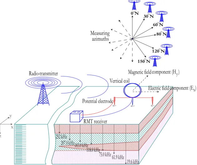
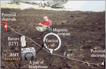
3.1.3 Scalar CHYN RMT Equipment 030
3.1.4 Radio-transmitters 032
3.2 Data Interpretation 033
3.2.1 Data Viewing 033
3.2.2 Data Transformation 036
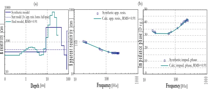
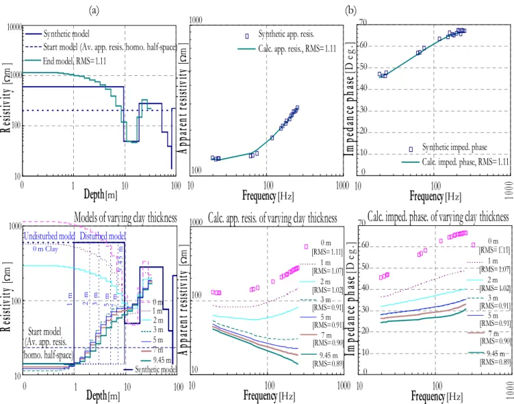
3.2.3 One-dimensional Inversion of Synthetic Data 037
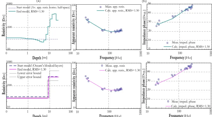
3.2.4 One-dimensional Inversion of Field Data 041
3.2.5 Two-dimensional Inversion of Field Data 051
3.2.5.1 Mesh Design and Verification 051
3.2.5.2 The Regularization Parameter 052
3.2.6 Nearby-topography Effect 062
4 Transient Electromagnetic Resistivity Models 069
4.1 Transient Electromagnetic Methods 069
4.1.1 Conceptual Background 069
4.1.2 Depth-of-investigation 070
4.1.3 Zonge Nano/ZeroTEM System 071
4.1.4 Data Deconvolution 074
4.1.5 Data Transformation 078
4.2 Data Interpretation 078
4.2.1 Data Viewing 078
4.2.2 One-dimensional Inversion of Synthetic Data 080
4.2.3 One-dimensional Inversion of Field Data 082
4.2.4 One-dimensional Joint-inversion of RMT and TEM Field Data 094
4.2.5 Three-dimensional Modeling of Synthetic Data 098
4.2.5.1 Grid Design and Verification 098
4.2.5.2 Model Geometry and Results 100
4.2.6 Nearby-topography Effect 106
4.3 Correlation of Surface Electromagnetic with Laboratory-based Resistivity Models 110 4.4 Geological Implications inferred from Surface Electromagnetic Resistivity Models 112
5 Laboratory-based Resistivity Models 114
5.1 Electrical Resistivity of Coal 114
5.2 Laboratory Methods for Measuring Resistivity 116
5.2.1 Conceptual Background 116
5.2.2 Samples and Terminal-configurations 118
5.2.3 Direct-current Measurements 120
5.2.4 Spectral Induced Polarization Measurements 121
5.3 Results and Interpretation 121
5.3.1 Resistivity Magnitude and Phase Angle Spectra 121
5.3.2 Argand Diagrams 122
5.3.3 IP Measures 124
5.4 Discussion 126
6 Summary and Conclusions 128
A Programs 136
B Mining Results 138
References 139
Acknowledgment 147
1
INTRODUCTION
1.1 Mining and Geophysics
Mining has been one of the oldest activities of man since times. As the human population increases and developing countries become more industrized, the search for new ore deposits will continue to grow. Evidence of the througness and diligence with which this search was conducted in olden times can be found in many places, such as the ancient workings in the Egyptian Eastern Desert to find and extract the Pharaoh's Gold [Harrell, 2002]. One must look for more ore where ore has already been found and in districts with natural conditions similar to those in the known district. Invasive techniques, such as expensive drilling and direct-sampling, can provide very accurate one-dimensional information about the subsurface, but only for the sampling location and for a limited volume of the subsurface. Here the geophysics − the study of physics of the Earth, Earth's materials and surrounding atmosphere
− enters the picture. A necessary condition for the detection of an ore body by geophysical (or non-invasive) methods is that the ore should differ sufficiently in physical properties (electric resistivity, magnetic susceptibility, bulk density, etc.) from that of the host background materials. The primary purpose of geophysics during the early stages in the life of a mine, i.e.
during the prospecting and exploration stages, is to separate areas which appear to be barren from those which appear to hold a promise of ore [Parasnis, 1973]. Consequently, the success of a well-conducted geophysical method is not to be measured by the number of ore bodies discovered or by the number of recommended boreholes that stuck ore, but by the time, effort and money which the survey has saved in eliminating ground which would otherwise have to be eliminated by more expensive methods.
Applied geophysics provides a wide range of very powerful methods which, when used correctly and in the right geological situations, will yield very useful information about the ground truth. Usually, multiple geophysical methods offer better answers than any individual method. During the last few decades, the hydrocarbon industry has exploited the geophysical exploration techniques to a far greater extent in terms of using the field data to quantify the value, size, and production capabilities of its resources. By contrast, the application of geophysical methods to mining industry, particularly to surface-mining, is not developed well in general [Nabighian and Asten, 2002]. Some possible reasons for this are:
(1) Insufficient knowledge by mining managers, engineers, and operators of the existence of geophysical methods, coupled with a high tech−high cost perception of geophysics.
(2) Perceived infrastructure and logistical difficulties in using geophysical methods due to the continuous mining activities.
(3) Lack of knowledge of the physical properties of the ore and host background materials which may be exploitable in a mining environment.
(4) Limited research effort applied to standard geophysical methods to develop higher- resolution acquisition or interpretation techniques applicable to mining problems.
(5) Scarcity of geophysicists with access to mine difficulties or with sufficient knowledge of mining culture or operational requirements to champion the use of geophysical methods in this area.
1.2 Electromagnetic Methods
Electromagnetic (EM) methods are among some of the oldest geophysical techniques, which involve the measurement of one (or more) electric and magnetic field components, at the earth surface (or in borehole), induced in the subsurface by a primary field produced from a naturally occurred (passive) or artificially generated (active) source of EM field. There are two competing families of methods: one family satisfies the diffusion equation, which ignores displacement currents and non-linear effects to obey the EM induction regime and operates at frequencies less than 1 MHz. The other family satisfies the wave equation, which considers displacement currents and operates frequencies above 1 MHz. The latter is beyond the scope of this work and will not be discussed further. Commonly, the term 'EM methods' tends usually to refer only to 'EM induction methods.' Because of the large number of EM methods, there are many ways of classifying them for discussion. One common classification, which will be used here, is to group by weather the EM data are measured in the frequency-domain (FD) or the time-domain (TD).
1.2.1 Frequency-domain Electromagnetic Methods
In a typical FDEM survey, EM energy is introduced into the ground as continuos waves by a small transmitting-coil, comprising few turns of wire around permeable core and carrying alternating-current (AC) and primary magnetic field of a fixed (or swept) frequency oscillation. Satisfying the physical laws of EM induction, the primary field spreads out in a three-dimensional space both above and below the ground and results in an induced (or eddy) current pattern in the ground, and hence an associated secondary magnetic field which is added to the primary field. The induced currents flow in such a way that their primary field opposes the secondary field. The strength of the secondary field depends, among other factors, upon the ground resistivity and excitation frequency of the primary field. Therefore, its amplitude, direction and phase differ from that of primary field and can yield information on the ground resistivity-distribution. Normally, the primary field is nulled by a closely (or widely) spaced small receiving-coil so that the in-phase (real) and out-of-phase (quadrature or imaginary) components of the secondary field are directly measured. Alternatively, the resultant (vector sum) of both primary and secondary fields is measured and the secondary is computed separately. Both transmitting- and receiving-coils are usually identical and tuned to the same frequency for sensible measurements. Geometrically, they are not only described as horizontal (vertical magnetic-dipole) or vertical (horizontal magnetic-dipole), but also as coplanar, coaxial (maximally-coupled) or orthogonal (minimally-coupled). The effective
depth-of-investigation is dependent of the weighted-average resistivity of the subsurface earth, operating frequency, transmitter−receiver spacing and the overall signal-to-noise ratio (SNR).
Among the FDEM methods are the magnetotelluric (MT) methods which involve simultaneous orthogonal measurements of two horizontal electric and three horizontal and vertical magnetic field components induced in the subsurface by primary fluctuating ionosphere currents by means of two electric-dipoles and three magnetic sensors respectively [Tikhonov, 1950; Cagniard, 1953]. Theses currents are due to the complex interaction of the solar-wind with the magnetosphere, i.e. geomagnetic micropulsations. Typically, MT methods operate at the frequency range between 0.001 and up to 10 Hz. The variability in amplitude and/or direction of the geomagnetic micropulsations requires more stacking time for improvement of the SNR, thus making MT methods expensive and low-productive. The MT measurements made at the audio-frequency range from 1 Hz to 10 kHz, using EM energy from distant-lightening discharges (or spherics) due to global thunderstorm activity, are generally referred to as audio-magnetotellruic (AMT), or controlled-sourceAMT (CSAMT).
Similarly, audio-frequency magnetic field (AFMAG) methods make use of this audio- frequency magnetic field, but the measured quantities are the azimuth and dip of the major axes of the polarization ellipse [Ward et al., 1968]. All these natural fields travel around the globe in the Earth's ionosphere waveguide cavity [Spies and Frischknecht, 1991], but are more frequent in equatorial regions such as Brazil, Central Africa and Malaysia. As the name implies, the controlled-source MT (CSMT) methods are those carry their own transmitters with prescribed characteristics, including loops, grounded dipoles or antennas.
Very low frequency (VLF) methods utilize EM radiation generated by remote powerful radio- transmitters which are distributed all around the world for the purpose of military communication and operate at frequency range from 10 to 30 kHz. These VLF transmitters emit continuously either superimposed frequency-modulated EM wave or occasionally choped unmodulated 'Morse code' [Paal, 1965; Watt, 1967]. The VLF antenna mast is effectively a long vertical wire (or rod) carrying an AC current, i.e. vertical electric-dipole. The signal strength is roughly proportional to the amplitude of electric field component parallel to the mast and to the mast length. A radiated EM wave consists of coupled vertical electrical and concentric horizontal magnetic fields, perpendicular to each other and to the direction of propagation. It travels efficiently over long distances in the Earth's ionosphere waveguide cavity. Neither the ground nor the ionosphere is a perfect conductor and some EM energy is lost into space or penetrates the ground. Without this penetration, there would be neither naval communication with submarines nor geophysical uses. Because the VLF electric field near the ground surface is titled, not vertical, it has also a horizontal component.
Induced currents in the ground by VLF magnetic field produce an opposite secondary magnetic field with the same frequency as the primary, but generally with a different amplitude and phase depending on the ground resistivity and excitation frequency of the primary field. The secondary magnetic field has also both horizontal and vertical components.
Any vertical secondary magnetic field component is by definition anomalous, causing a tilted or elliptically polarized resultant field. A VLF magnetic field can be sensed by a small induction coil in which current flow in proportion to the core permeability, number-of-turns and the magnetic field component along its axis. Most VLF equipment compares vertical with horizontal magnetic fields either directly or by measuring the tilt-angle which is initially inferred from the in-phase and quadrature components.
In VLF work the profile direction is almost irrelevant, the critical parameter being the relationship between the known (or presumed) geological strike of a subsurface conductor and the azimuth (or bearing) of the radio-transmitter. A subsurface conductor which strikes towards the radio-transmitter is well-coupled, as the magnetic field is at right angle to it and current can flow freely. Otherwise, the current flow would be restricted, reducing the strength of the secondary field. The measuring procedure for a VLF survey is rather simple, carried out as follows: the VLF receiver (a small hand-held device) is tuned to a particular frequency of the selected radio-transmitter. The azimuth of the radio-transmitter is obtained by rotating a small induction coil around a vertical axis until the null position (i.e. minimum audibility) is found. The coil is then rotated around a horizontal axis at right angle to that azimuth, where the tilt-angle is noted at the null position. Measurements are then performed along the survey profile at right-angle to that azimuth using only a single, well-defined frequency. The asymmetry of the tilt-angle data along a profile can be used to obtain a qualitative estimate of the dip of a subsurface conductor, if present.
Very low frequency−resistivity (VLF−R) methods are hybrid forms of electrical and EM methods [Scott, 1975; Fischer el al., 1983], but still similar in principles to the conventional VLF methods with two significant differences. First, the horizontal resultant electric field component is measured by the voltage drop between a pair of potential electrodes planted into the ground. Whereas, the horizontal resultant magnetic field component is sensed by a small vertical induction coil at the mid-point between electrodes. Second, the measured quantities are commonly expressed in terms of the apparent resistivity and impedance phase (the phase lag in time of the measured electric field relative to magnetic field) at the frequency range between 10 and up to 30 kHz. This allows a semi-quantitative interpretation to be performed.
Radiomagnetotelluric (RMT) methods are extension of VLF−R methods to higher frequency range up to 1MHz, although the applicable frequency range of most RMT equipment is limited between 10 and 300 kHz [Turberg et al., 1994; Turberg and Barker, 1996]. Recently, an impressive work was devoted by the Center of Hydrogeology Neufchâtel (CHYN) at the University of Neufchâtel in Switzerland to establishing a new VLF methodology known as Very low frequency−resistivity EM gradient (VLF−EM GRAD) methods [Bosch and Müller, 2001]. These techniques reveal high vertical and horizontal ground resistivity-resolution. The horizontal resultant magnetic field component is sensed simultaneously and continuously at two different altitudes, above the ground, with two attached vertical induction coils centrally- spaced 1 m apart. The signal differences in both in-phase and quadrature components between the upper and lower coils, which are based on their mutual coupling, are usually measured in percentage.
Slingram methods utilize two transmitting- and receiving-coils separated by a fixed distance, typically 30 to 350 m, and moved simultaneously over the survey area [Parasnis, 1973]. The ratio of the vertical secondary to primary magnetic field amplitudes is determined at several frequencies. This is initially done from measurements of both in-phase and quadrature components, which in turn are dependent on the mutual coupling between the two coils.
Slingram is synonymous with the horizontal loop EM (HLEM) methods. Ground conductivity meters(GCM)are portable EM instruments which directly measure the terrain conductivity at shallow depths [McNeill, 1980; Frischknecht et al., 1991]. They are essentially Slingram systems, but the operating frequency is sufficiently low, typically 0.5 to 10 kHz at each measuring inter-coil spacing, so that the skin-depth in the ground is always significantly
greater than this spacing. That means, the measurements must be made at low induction number (ratio of the inter-coil spacing to skin-depth). Virtually all response from the ground is in the quadrature phase of the received signal. So, quadrature component is taken to be a linear measure of the apparent conductivity of the ground. The in-phase component is measured in parts per thousand. The GCM devices can be deployed both horizontally and vertically. When used as a horizontal-coil system (vertical dipole mode), the device is quite sensitive to the relatively low-conductive steeply dipping subsurface structures. Whereas, as a vertical-coil system (horizontal dipole mode) the device is insensitive to such structures and gives fairly accurate measurement of ground conductivity in close proximity to them.
Sundberg methods utilize a horizontal dipole source as transmitter, typically an insulated- cable of few hundred meters to several kilometers long grounded at both ends or long rectangular loop, and a small receiving-coil. Phase reference is determined by a feeding coil located close to the transmitter cable or loop using a compensatory system. Measurements are usually made at the right angle to the cable or long-side of the loop [Parasnis, 1991]. Turam methods are further development of the Sundberg methods in which the feeding coil is not present, and therefore there is no need to carry phase reference information from the transmitter. Additionally, they utilize two mobile receiving-coils which are separated by, and deployed successively with, a fixed distance of about 10 to 20 m. The two coils provide a mean whereby the horizontal gradient of amplitude ratio of the vertical secondary field (or phase difference) at each two successive points can be determined. This is initially done from measurements of both in-phase and quadrature components, which in turn are dependent on the mutual coupling between the two coils. The major advantages from using such fixed- source methods over moving-source methods, i.e. Slingram and GCM, are that the topography has a less significant effect on their data, as well as the EM coupling between the cable (or loop) and the subsurface is maintained constant throughout the survey profile. Although in both fixed- and moving-source methods the receiving-coils are usually held horizontally, they can be deployed in three mutually perpendicular planes, and hence the EM field components can be measured completely.
Magnetometeric resistivity (MMR) methods utilizes a commutated direct-current (DC) (alternating square-waveform) injected into the ground through a pair of widely separated electrodes. The anomalous resistivity is determined at the mid-point by measuring the secondary magnetic field arising from the non-inductive currents using an extremely sensitive low-noise magnetometer aligned perpendicular to the line between the electrodes [Edwards and Nabighian, 1991]. The electrode spacing may be held fixed or it may be increasingly varied to obtain much depth-of-investigation. They are used to explore beneath a highly- conductive surficial layer. Yet, they met with little success. Generally speaking, the claimed depth-of-investigation possible with the passive FDEM methods is much greater than that of the active FDEM methods.
1.2.2 Time-domain Electromagnetic Methods
In a typical TDEM survey, EM energy is introduced into the ground as transient pulses, instead of continuous waves, by a large transmitter-loop carrying steady1 current and primary magnetic field. Satisfying the physical laws of EM induction, immediately after the current and primary field are suddenly turned-off, an associated secondary magnetic field resulting from an induced current pattern in the ground is sensed by a small receiver-loop and decays with time as the current gradually dissipates. The induced currents flow in such a way that
1Either pure DC or commutated DC or low-frequency AC (typically 20 to 50 Hz) current.
their primary field opposes the secondary field. The strength of the secondary field depends, among other factors, upon the ground resistivity and sampling time of the transient-decay response. Therefore, its amplitude and shape yield information on the ground resistivity- distribution. Normally, the recorded signal by the receiver is the time-derivative of the decay of vertical secondary magnetic field as a voltage. The TDEM methods can be used in a number of different transmitter-receiver configurations. The most common loop-loop configurations are frequently described as in-loop (central loop), coincident loop, single (common) loop, separate loop, dual loop and fixed transmitter-/roving receiver-loop [Nabighian and Macnae, 1991]. The effective depth-of-investigation is dependent of the weighted-average resistivity of the subsurface earth, sampling time and transmitter-dipole moment (the effective area times output-current) and the overall SNR [Spies, 1989].
Long offset transient EM (LOTEM) is a subgroup of the TDEM methods in which carefully controlled electric current, usually several tens of amperes, is driven through the earth by means of a horizontal dipole source as transmitter, typically an insulated-cable of 1 to 2 km long grounded at both ends [Kaufman and Keller, 1983; Strak, 1992]. The transmitter is kept fixed, while many different mobile receivers about the survey area are used to measure two horizontal electric field components and the time-derivative of the vertical magnetic field component as voltages. The transmitter−receiver distance, called offset, is comparable to the depth-of-investigation, which is the reason for calling the method long offset TEM. It usually varies between 2 and 20 km, shorter or longer offsets are also possible, but are less often used.
The LOTEM methods are now gaining recognition among geophysicists because of the possibility of overcoming typical EM noise problems as well as obtaining higher depth resolution with better transmitter signature.
For both FDEM and TDEM surveys, the primary field amplitude is decreased exponentially with depth and secondary field amplitude produced in the ground is similarly attenuated on its way to the surface, i.e. both surveys are skin-depth and diffusion-depth limited respectively.
The TDEM surveys have principal advantages over the FDEM survey of that the primary magnetic field is not present during the measurement of the secondary magnetic field and that simultaneous voltage measurements of secondary field as a function of time are equivalent to quadrature component measurements over a very broad frequency range. Therefore, more depth-of-investigation would be expected in TDEM surveys, although the exact depth is not known. The absence of a primary field during TDEM measurements allows the receiver-loop to be positioned within the transmitter-loop, a technique which can be used in any FDEM work only with a very large transmitter-loop because of the strong coupling to the primary field. Furthermore, the TDEM surveys have a relatively low productivity because of long recording time. This is partly due to more stacking time for improvement of the SNR, especially at later-times. Contrary to FDEM, the TDEM measurements must be conducted over a longer period of time, causing the amplitude of the secondary field to vary much more.
That means, the TDEM system must have a wide dynamic-range.
Like any other geoelectric methods, EM induction surveys can be conducted in the form of either vertical sounding or horizontal profiling. Assuming an uniform horizontally layered- earth, EM sounding is designed to determine variations in the ground resistivity with depth.
Measurements are usually made at a number of frequencies or sampling times using a fixed transmitter−receiver spacing [Spies and Frischknecht, 1991]. Alternatively, measurements can be made at a single frequency or sampling time by varying the transmitter−receiver spacing.
The first technique is sometimes is called parameteric sounding, while the second is called geometric sounding. On the other hand, EM profiling is designed to determine variations in
the ground resistivity laterally. Measurements are also made at a single frequency or sampling time wherein a fixed transmitter−receiver spacing is moved progressively along a traverse to create a horizontal profile [Frischknecht et al., 1991].
By comparison, most EM methods have a major advantage over the electrical methods, including DC resistivity, self-potential (SP) and induced polarization (IP), is that the induction process does not require direct (galvanic) electrode-contact with the ground. Consequently, the data can be acquired relatively more quickly than with electrical methods. The induction process also allows the EM methods to be conducted from the aircraft and ships, as well as down boreholes. Because EM soundings depend only on the longitudinal conductivity of an uniform horizontally layered-earth, whereas DC resistivity soundings, as an example, depend on both transverse and longitudinal resistivities [Spies and Frischknecht, 1991]. Thus, over an uniform horizontally layered-earth, DC resistivity soundings can provide better vertical resolution than EM soundings, especially for the resistive layers. However, over a laterally varied conductive (or fairly resistive) earth, EM soundings can generally provide better vertical and lateral resolution than DC resistivity soundings. Although modern EM equipment tends to be somewhat more costly, considering its sophistication, EM methods are still highly sensitive to the background natural EM and cultural noise [Spies and Frischknecht, 1991].
Whereas, electrical methods are less expensive and relatively insensitive to such background noise. Unlike the case for EM soundings, data processing and mutli-dimensional interpretation of electrical soundings are straight forward. Multi-dimensional EM interpretation may be used preferentially, but still require large amount of computing time and are limited by the computational difficulties in defining especially two- and three-dimensional models.
A much more comprehensive and detailed discussion of the various EM methods, with exception of the ground penetrating radar (GPR), has been produced by Misac Nabighian [1988, 1991] and co-authors. In the framework of present work, we shall come to touch on only two particular ground-based EM approaches that fall under the headings of radiomagnetotelluric (RMT) and transient EM (TEM) depth-sounding methods, and do not look deeper in other methods. The former is a passively FDEM method, whereas the second is an actively TDEM method. Both are among some of the robust near-surface exploration techniques that have been successfully used in areas as diverse as environmental [Zacher et al., 1996; Tezkan et al., 1996; Hördt et al., 1999; Newman et al., 2003], hydrogeological [Fitterman and Stewart, 1986; Christensen and Sørensen, 1998; Turberg et al., 1994; Bosch and Gurk, 2000] and mineral investigations [Scott, 1975; Palacky, 1983; Asten, 1987; Helwig et al., 1994].
Since the 1990's, the Institute of Geophysics and Meteorology (IGM) at the University of Cologne has continuously concentrated on the application and development of RMT/TEM methodology and interpretation schemes. Despite the reasons given in Section 1.1, which have always restricted the geophysical applications in the area of surface-mining, growing competition from other energy sources in Germany, such as imported hard coal, made it essential for RWE-Power AG to minimize costs, especially in field-work functions like expensive drilling and direct-sampling. Therefore, close cooperation of RWE-Power AG with experts, universities, institutions and associations was maintained for the purpose of continuously establishing cost-effective exploration strategies at the Rhineland opencast mines. On the other hand, there was an increasing interest of the IGM-Cologne to highlight the applicability, efficiency and reliability of RMT and TEM methods in an area like brown coal exploration. Both reasons greatly encouraged the field survey to get started.
1.3 Scope and Objectives of the Present Work
The present study was devoted to carrying out RMT and TEM investigations over the shallow coal seams at the opencast mine 'Garzweiler I', northwest of Cologne. It was hoped that such methods may image the vertical electrical resistivity structure of these seams, and hence define much better estimates of their boundaries and unexpected changes in their altitudes or thicknesses (faulting, dipping, thinning, etc.) which are usually considered as geological surprises for mining community, if present. For this purpose, the steps in planning the field campaign were as follows:
(1) Collecting the available topographic, geological and geophysical information about the areas concerned to find out what type of rocks we are likely to encounter within them and how they are likely to be interrelated.
(2) For deciding whether the RMT and TEM methods can be usefully undertaken within the survey areas or not, a two-day trial survey ought to be carried out before launching a large- scale field operations. Such a survey, together with a preliminary forward modeling, helped us to form some idea about the EM responses predicted from the various rocks within the areas, as well as those expected from nearby-topography. It also indicated some specific modifications necessary in the measurements for optimizing survey design, and hence obtaining the best possible results.
(3) Staking the survey areas before starting the measurements to establish a coordinate system in which every sounding center was clearly and uniquely marked. This enabled us to reoccupy exactly the same sounding center with both RMT and TEM measurements so that a comparison of their resistivity models is rendered reliable. This was performed using a theodolit and differential GPS1 readings, as well as using tap measures and some wooden sticks.
(4) It was really a sound policy to procure some representative rock samples from the survey areas and measure their electrical properties in the laboratory to determine what can be interpreted reliably from surface RMT and TEM measurements.
This dissertation consists of six chapters and two appendices. Its structure is as follows: this chapter contains general introductory sections which state how the link between mining and geophysics comes into play, explain where RMT and TEM methods are placed in applied electromagnetics and discusses the scope and objectives of the present work. They also outline the importance and geological background of the Rhineland brown coal and describe the survey areas at the opencast mine 'Garzweiler I.' Chapter 2 gives an introduction to the inversion of EM data. Special attention is given to the one-dimensional (1D), two-dimensional (2D) and three-dimensional (3D) RMT/TEM inversion and modeling schemes which have been used in the present work. Chapter 3 explains the conceptual background of RMT methods and gives detailed description on how to acquire azimuthal RMT data sets in the field and to interpret them reliably in terms of 1D and 2D resistivity models. During the course of this chapter, the effect of nearby-topography on the RMT data is qualitatively assessed. Similar to RMT methods, the conceptual background of TEM methods and detailed description on how to acquire segmented in-loop Nano/ZeroTEM data sets in the field and to interpret them reliably in terms of 1D and 3D resistivity models are described in Chapter 4.
The effect of nearby-topography on the TEM data is qualitatively assessed. It is an end intention of this chapter to correlate the final 1D/2D RMT and 1D/3D TEM earth models with laboratory-based resistivity models, which represent almost the whole vertical succession at the survey areas, and to give some useful geological implications inferred from these models.
1Global positioning system.
Note that the final RMT and TEM resistivity models are visualized as two-dimensional section- or plane-views because the end objective of such investigation work is a practical guide for mining industry. Apart from the particular focus on the RMT and TEM methods, Chapter 5 illustrates two direct methods for measuring the electrical resistivity of rock samples in the laboratory, namely DC and spectral induced polarization (SIP) techniques. Like any other petrophysical analysis, the chapter first reviews the published resistivity ranges of coal among the most common sediments, ores and ore minerals. Then, it describes in details the studied rock samples and terminal-configurations used for both measuring techniques.
Later on, the final results and interpretation, as well as a brief discussion are given. Finally, Chapter 6 summarizes the main concluding remarks that could be drawn from the whole research. A brief review about the programs used for data processing, inversion/modeling and visualizations are given in Appendix A. Mining results of the Garzweiler Coal Seam versus the interpreted 1D/2D RMT resistivity models, along profile I at the 'Coal-covered Area', are given in Appendix B.
1.4 Rhineland Brown Coal
The largest single lignite2, or brown coal, deposit in Europe is found in Rhineland which covers an area of some 2,500 km2 to the northwest of Cologne. Since lignite is the youngest variety of all coals, built in Early to Middle Miocene age [26.60 Ma], overlain by more recent sand, gravel, and clay, and thus closer to the surface, it is mined in large-scale opencast mining. Lignite seams also extend to a depth of around 500 m, while overburden thickness can be up to 300 m.
Cologne-based RWE-Power AG (formerly RWE-Rheinbraun AG) is responsible for mining of lignite in Rhineland with an annual production of around 100 million metric tons. It operates four large opencast mines, namely 'Inden I/II', 'Garzweiler I', 'Hambach I' and 'Bergheim.' The 'Garzweiler I' mine (Figures 1.1 and 1.2) accounts for one-third of total lignite output. The planned 'Garzweiler II' mine will replace capacity from 'Bergheim' mine, which is nearly worked out. Approximately one-quarter of the public electricity supply in Germany, generated by the coal-fired power plants of RWE-Energie AG, is based on the Rhineland brown coal [RWE AG Group, 1989].
Because of their depth below groundwater level (up to 500 m) and due to their horizontal extension (several kilometers wide and long), Rhineland opencast mines require extensive dewatering and flood control systems, both aimed at preventing in-mine flooding and guarantee dry mining. RWE-Power mining activities generally start with the central removal (or stripping) of overburden utilizing a fleet of giant bucket-wheel excavators. This is followed by mining the uppermost flat-laying lignite seams, then interburden to uncover further lignite seams separately. Once mined-out, lignite masses are entirely transported via conveyor belt systems or railways to the nearby refineries and, later on, to the coal-fired power plants. In an environmental move, RWE-Power AG carries out immediate reclamation of both outside waste dumps and mined-out areas of the opencast mines as part of its normal operations. Problems in recultivation are occurred due to minor ground-grade that makes reforesting difficult.
2A weakly-consolidated sedimentary rock, formed by the partial decomposition of woody plant debris (or peat), under moderately-high temperature and pressure, over geologic time. This low-rank (or low-carbonized) coal has a high inherent moisture content, sometimes as high as 45 percent, and a relatively low heat/energy content, from 9 to 17 million BTU (British thermal unit) per ton. It is used exclusively as fuel for steam-electric power plants [Matthes, 1990].
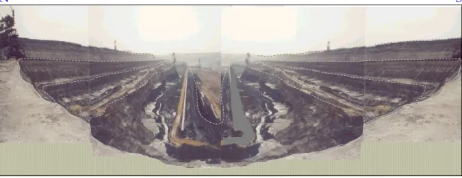
N S
Figure 1.1: Field panorama of the opencast mine 'Garzweiler I', northwest of Cologne, viewed end- on from the western side.
1.5 Geological Background of Rhineland
The Cenozoic Dutch−German rift system transects the Rhenish Shield, that comprises the Rhenish Massif in the north and the Black Forest in the south, to form the 100 km long and 50 km wide Lower Rhine Embayment in Germany [Schäfer et al., 1996; Wong et al., 2001]. This asymmetrical basin (or graben) is subsided along NW−SE oriented faults (Figure 1.2a), forming several tectonic blocks: the Rur, Venlo, Erft, Krefeld and Köln blocks [Klett et al., 2002]. The entire rift sedimentary section (Figure 1.2b) consists of the Tertiary and Quaternary unconsolidated fill of a maximum thickness of more than 1500 m and unconformably rests on a pre-existing Mesozoic to Paleozoic basement.
The tectonic−geological events which accompanied the formation of the Rhineland lignite merit special considerations. In the Paleocene, the area of the Lower Rhine Basin remained largely sediment-free. From the Early to Middle Oligocene the area was confined to tightly circumscribed sinking at differing speeds and depths. Furthermore, the old (Tertiary) North Sea could transgressed onto the basin with a huge carpet of floating peat, provided from the heights of the Rhenish Massif [Zagwijn, 1989]. This received fresh water from the south through a wide river, the old Rhine, and consequently caused the peat to sink into the rift trench. During the climax of the marine transgression in the Late Oligocene, the entire rift marine sediments were extensively deposited and covered by these accumulated organic masses that became the rich lignite seams since the Early Miocene regression of the North Sea. The extensive drift lignite horizons and the lateral change from lignite to sand represent a radical change in the depositional environment that resulted from short-lived transgressions of the North Sea onto the freshwater swamps [Shäfer et al., 1996]. It is believed that the Rhineland coal seams, i.e. Garzweiler, Frimmersdorf and Morken seams, formed in this way.
They join up in the center of the basin to form one 'Main Seam' which reaches a maximum thickness of about 100 m (Figure 1.2b). At the end of Late Miocene and during the Pliocene, thick and coarse-grained fluvial sediments followed the stepwise regression of the sea.
Finally, the Pleistocene uplift of the Rhenish Massif increased the subsidence of the Lower Rhine Basin to form the early Rhineland plains.
(a)
A
B
MASSIF RHENISH
MASSIF RHENISH
MASSIF RHENISH Rur
Feld biss Peel
Erft Fau
lt
Fau lt Fau
lt
Fau lt
Blo ck Erft
Ru r Blo
ck Ven
lo B lock
Kre feld
Blo ck
Blo ck Kö
ln
II I
Inden
Ville Frechen
Hambach
Bergheim Fortuna II I
Garzweiler Rur
Ruhr
Wupper
Erft Niers
Maas
Rhine
Sieg Roermond
Venlo Krefeld
Düsseldorf M./Gladbach
Aachen D
üren
Euskirchen Cologne
Bonn
2510
2550
5630 70
56 2550
2510
70
56
30
56
[km]Y Coordinates
X Coordinates[km]
LOWER RHINE EMBAYMENT
Present, former and future opencast mines
Rur Block Erft Block K öln Block
SW
Inden mine Hambach mine Bergheim mine
400 m 0
0 4000 m
NE
A B
Pleistocene Pliocene Miocene Oligocene Lignite [Brown coal]
Mesozoic basement
(b)
Figure 1.2: (a) Location of the opencast mine 'Garzweiler I', northwest of Cologne, within the Lower Rhine Embayment and (b) idealized geological cross-section running SW−NE though the Rur, Erft and Köln tectonic blocks with tentative Cenozoic stratigraphy. Some opencast mines are projected onto the section [redrawn after Klett et al., 2002]. Coordinates of the location map are given by the German national (Gauss−Krüger) coordinate system.
1.6 Survey Areas
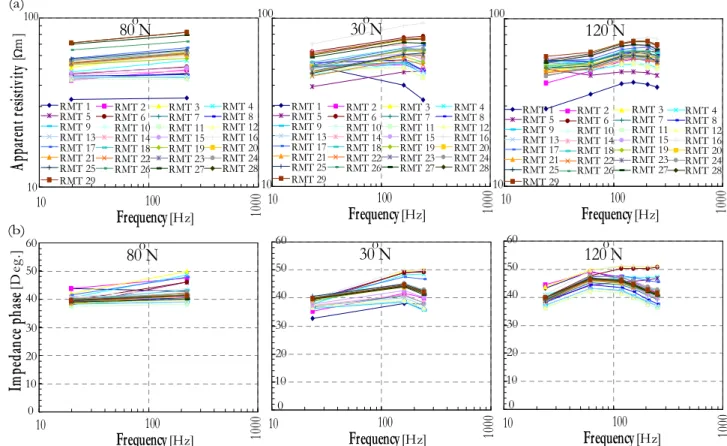
A total of 86 azimuthal RMT and 33 in-loop TEM soundings were carried out along six separate profiles between April and May 2002 over two opencast benches (or terraces) at the opencast mine 'Garzweiler I', with a permanent crew of two persons. Throughout this dissertation, these small-scale benching areas are always referred to as 'Coal-covered Area' and 'Sand-covered Area.' The 'Sand-covered Area' is located at relatively higher altitude to the northeast of the 'Coal-covered Area' and bordered on the northerly side by a large hillock (about 22.8 m high) (Figure 1.3a). This hillock consists mainly of sand, gravel and loam.
Profile I (about 350 m long) is conducted parallel to, and fare as enough as possible from, that hillock and directed 90o N, while profile II (about 60 m long) is almost perpendicular to it.
The topography along each profile is almost of very flat relief, where the elevation-difference does not exceed 0.45 m. Soundings RMT 1 and TEM 1 are close to the stratigraphic-control borehole 'WS 1452' and considered as control soundings.
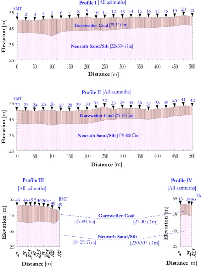
The 'Coal-covered Area' is bordered on the northerly side by a small hillock (about 8 m high) and edged on the southerly side with a very steep cliff (about 26 m deep) to another subjacent mining bench (Figure 1.3b). This hillock consists of the uppermost (non-mined) Garzweiler Coal and Surface Sand. Profiles I and II (each about 500 m long) are conducted parallel to, and fare as enough as possible from, both the hillock and the cliff and directed 79o N, while profiles III and IV (120 m and 32.5 m long respectively) are almost perpendicular to them.
The area displays a slightly rugged topographic-relief, the elevation-difference varies between 0.05 and 3.5 m. Soundings RMT 32 and TEM 17 are close to the stratigraphic-control borehole 'WS 1380' and considered as control soundings.
Along the main parallel profiles, RMT soundings are performed at regular spacings, between centers, of about 12.5 m and 25 m for the 'Sand-covered Area' and 'Coal-covered Area' respectively, while TEM soundings are always spaced 50 m apart. Spacings along the complementary perpendicular profiles are a little irregular and shorter. Although profile locations were selected to fulfill the survey objectives, logistical difficulties due to the continuous mining activities and taking into account considerations of nearby-topography effect to minimize its distortion on the EM data, limited, to some extent, the number of profiles within each survey area.
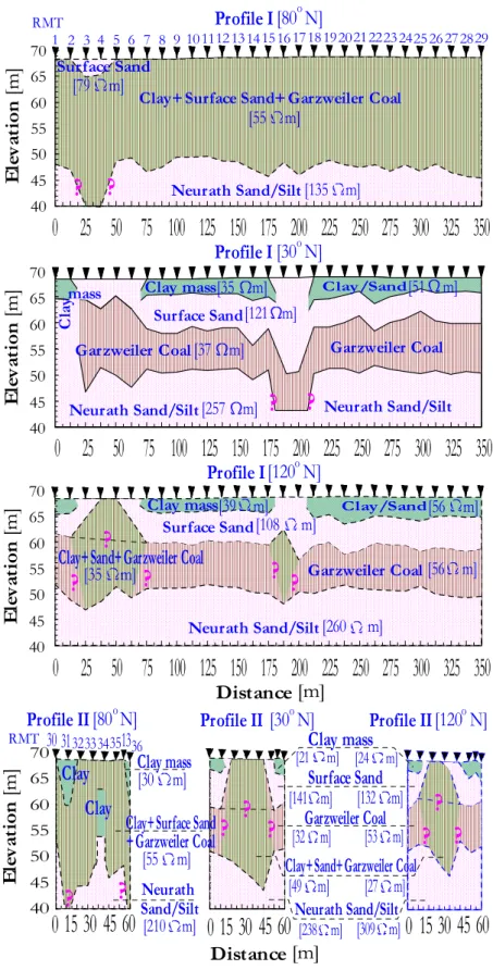
The local stratigraphy at the survey areas typically comprises a layer-cake sequence, from top to bottom, of Garzweiler, Frimmersdorf and Morken Coals embedded in a sand background, consisting of Surface, Neurath, Frimmersdorf and Morken Sands (Figure 1.4). A considerable amount of clay and silt intervenes the whole succession. At the 'Coal-covered Area', the uppermost part of Garzweiler Coal (about 5 m thick) is already mined-out prior to the field measurements.
Profile IV
Profile III Profile II
Profile I
TEM 17
RMT 32 TEM 25 RMT 50
RMT 49 TEM 24 TEM 22
RMT 43
TEM 21 RMT 42
TEM 12 RMT 22
TEM 11 RMT 21
RMT 1 TEM 1
Borehole ID: WS1380
TEM (b) RMT
RMT 36 TEM 8
RMT 29
RMT 1 TEM 1
RMT 30
Borehole ID: WS1452
TEM (a) RMT
Figure 1.3: Topographic-relief models and locations of RMT/TEM soundings and stratigraphic- control boreholes at the survey areas: (a) 'Sand-covered Area' and (b) 'Coal-covered Area'.
Coordinates are given by the German national (Gauss−Krüger) coordinate system.