8.1 Singular Value Decomposition (SVD)

Exercise 8: Frequency Response of MIMO Systems

8.1 Singular Value Decomposition (SVD)

The Singular Value Decomposition plays a central role in MIMO frequency response analysis.

Let’s recall some concepts from the course Lineare Algebra I/II: 8.1.1 Preliminary Definitions

The induced norm||A||of a matrix that describes a linear function like

y=A·u (8.1)

is defined as

||A||= max

u6=0

||y||

||u||

= max

||u||=1||y||.

(8.2)

Remark. In the course Lineare Algebra I/II you learned that there are many different norms and the expression ||A|| could look too generic. However, in this course we will always use the euclidean norm ||A||=||A||2. This norm is defined as

||A||2 =√ µmax

=p

maximal eigenvalue of A^∗·A (8.3) where A^∗ is the conjugate transpose or Hermitian transpose of the matrix A. This is defined as

A^∗ = (conj(A))^T (8.4)

Example 1. Let

A=

1 −2−i 1 +i i

.

Then it holds

A^∗ = (conj(A))^T

=

1 −2 +i 1−i −i

T

=

1 1−i

−2 +i −i

.

Remark. If we deal withA∈R^n×m holds of course

A^∗ =A^T. (8.5)

One can list a few useful properties of the euclidean norm:

(i) Remember: A^T ·A is always a quadratic matrix!

(ii) IfA is orthogonal:

||A₂||= 1. (8.6)

(iii) IfA is symmetric:

||A₂||= max(|e_i|). (8.7)

(iv) If A is invertible:

||A⁻¹||2 = 1

õ_min

= 1

√minimal eigenvalue of A^∗·A

(8.8)

(v) If A is invertible and symmetric:

||A⁻¹||₂ = 1

min(|ei|) (8.9)

where e_i are the eigenvalues of A.

In order to define the SVD we have to go a step further. Let’s consider a Matrix A and the linear function 8.1. It holds

||A||² = max

||u||=1y^∗·y

= max

||u||=1(A·u)^∗·(A·u)

= max

||u||=1u^∗·A^∗·A·u

= max

i µ(A^∗·A)

= max

i σ_i².

(8.10)

where σ_i are thesingular values of matrix A. They are defined as σ_i =√

µ_i (8.11)

where µi are the eigenvalues of A^∗·A.

Combining 8.2 and 8.11 one gets

σ_min(A)≤ ||y||

||u|| ≤σ_max(A). (8.12)

8.1.2 Singular Value Decomposition

Our goal is to write a general matrix A ∈C^p×m as product of three matrices: U, Σ and V. It holds

A=U·Σ·V^∗ with U ∈C^p×p, Σ∈R^p×m, V ∈C^m×m (8.13) Remark. U and V are orthogonal, Σ is a diagonal matrix.

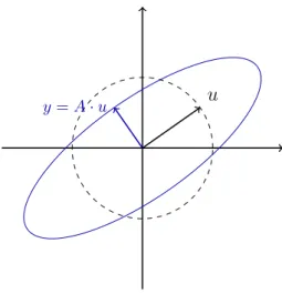
y=A·u u

Figure 1: Illustration of the singular values.

Kochrezept:

LetA ∈C^p×m be given:

(I) Compute all the eigenvalues and eigenvectors of the matrix A^∗·A∈C^m×m

and sort them as

µ1 ≥µ2 ≥. . .≥µr > µr+1 =. . .=µm = 0 (8.14) (II) Compute an orthogonal basis from the eigenvectors v_i and write it in a matrix as

V = (v₁ . . . v_m)∈C^m×m (8.15) (III) We have already found the singular values: they are defined as

σi =√

µi fori= 1, . . . ,min{p, m}. (8.16) We can then write Σ as

Σ =







σ₁ 0 . . . 0

. .. ... ... σ_m 0 . . . 0





 ∈R^p×m, p < m (8.17)

Σ =



















 σ₁

. ..

σ_n 0 . . . 0

... ... 0 . . . 0





















∈R^p×m, p > m (8.18)

(IV) One finds u₁, . . . , u_r from u_i = 1

σi

·A·v_i for all i= 1, . . . , r (for σ_i 6= 0) (8.19)

(V) If r < p one has to complete the basis u1, . . . , ur (with ONB) to obtain an orthogonal basis, with U orthogonal.

(VI) If you followed the previous steps, you can write A=U ·Σ·V^∗ Motivation for the computation of Σ, U und V.

A^∗·A = (U ·Σ·V^∗)^∗ ·(U ·Σ·V^∗)

=V ·Σ^∗·U^∗·U ·Σ·V^∗

=V ·Σ^∗·Σ·V^∗

=V ·Σ²·V^∗.

(8.20)

This is nothing else than the diagonalizationof the matrixA^∗·A. The columns ofV are the eigenvectors of A^∗·A and the σ²_i the eigenvalues.

ForU:

A·A^∗ = (U ·Σ·V^∗)·(U ·Σ·V^∗)^∗

=U ·Σ·V^∗·V ·Σ·U^∗

=U ·Σ^∗·Σ·U^∗

=U ·Σ²·U^∗

(8.21)

This is nothing else than the diagonalizationof the matrixA·A^∗. The columns ofU are the eigenvectors of A·A^∗ and the σ²_i the eigenvalues.

Remark. In order to derive the previous two equations I used that:

• The matrix A^∗·A is symmetric, i.e.

(A^∗·A)^∗ =A^∗·(A^∗)^∗

=A^∗·A.

• U⁻¹ =U^∗ (because U is othogonal).

• V⁻¹ =V^∗ (because V is othogonal).

Remark. Since the matrix A^∗ ·A is always symmetric and positive semidefinite, the singular values are always real numbers.

Remark. The MATLAB command for the singular value decomposition is [U,S,V]=svd

One can write A^T as A.’=transpose(A) and A^∗ as A’=conj(transpose(A)). Those two are equivalent for real numbers.

Remark. Although I’ve reported detailed informations about the calculation of U and V, this won’t be relevant for the exam. It is however good and useful to know the reasons that are behind this topic.

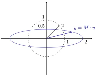
Example 2. Let u be

u=

cos(x) sin(x)

with ||u||= 1. The matrix M is given as

M = 2 0 0 ¹₂

!

We know that the product of M and u defines a linear function y=M·u

= 2 0

0 ¹₂

!

·

cos(x) sin(x)

= 2·cos(x)

1

2 ·sin(x)

! .

We need the maximum of ||y||. In order to avoid square roots, one can use that the x that maximizes||y||should also maximize ||y||².

kyk² = 4·cos²(x) + 1

4 ·sin²(x) has maximum

d||y||²

dx =−8·cos(x)·sin(x) + 1

2·sin(x)·cos(x)= 0^!

⇒ x_max=

0,π 2, π,3π

2

.

Inserting back for the maximal ||y|| one gets:

||y||_max= 2, ||y||_max= 1 2. The singular values can be calculated with M^∗·M:

M^∗·M =M^|·M

=

4 0 0 ¹₄

⇒ λ_i =

4,1

4

⇒ σ_i =

2,1

2

.

As stated before, one can see that||y|| ∈[σ_min, σ_max]. The matrixU has eigenvectors of M·M^| as coulmns and the matrixV has eigenvectors of M^|·M as columns.

In this case

M·M^| =M^|·M,

hence the two matrices are equal. Since their product is a diagonal matrix one should recall from the theory that the eigenvectors are easy to determine: they are nothing else than the standard basis vectors. This means

U = 1 0

0 1

, Σ =

2 0 0 ¹₂

, V =

1 0 0 1

.

Interpretation:

Referring to Figure 2, let’s interprete these calculations. One can see that the maximalampli- fication occurs atv =V(:,1) and has direction u=U(:,1), i.e. the vectoru is doubled (σmax).

The minimal amplification occurs at v =V(:,2) and has direction u =U(:,2), i.e. the vector u is halved (σ_min)

u y =M ·u

2 1

1 0.5

Figure 2: Illustration von der Singularwertzerlegung.

Example 3. Let

A=





−3 0 0 3

√3 2





be given.

Question: Find the singular values ofA and write down the matrix Σ.

Solution. Let’s computeA^TA:

A^TA=

−3 0 √ 3

0 3 2

·





−3 0

0 3

√3 2



=

12 2√ 3 2√

3 13

One can see easily that the eigenvalues are

λ₁ = 16, λ₂ = 9.

The singular values are

σ1 = 4, σ2 = 3 We write then

Σ =



 4 0 0 3 0 0



.

Example 4. A transfer function G(s) is given as

1 s+3

s+1 s+3 s+1 s+3

1 s+3

!

Find the singular values of G(s) at ω= 1^rad_s .

Solution. The transfer function G(s) evaluated atω = 1^rad_s has the form G(j) =

1 j+3

j+1 j+3 j+1 j+3

1 j+3

!

In order to calculate the singular values, we have to compute the eigenvalues of H =G^∗·G:

H =G^∗·G

=

1

−j+3

−j+1

−j+3

−j+1

−j+3 1

−j+3

!

·

1 j+3

j+1 j+3 j+1 j+3

1 j+3

!

=

3 10

2 10 2 10

3 10

!

= 1 10·

3 2 2 3

.

For the eigenvalues it holds

det(H−λ·1) = det

3

10−λ ₁₀²

2 10

3 10 −λ

!

= 3

10−λ 2

−

− 2 10

2

=λ²− 6

10λ+ 5 100

=

λ− 1 10

·

λ− 5 10

.

It follows

λ₁ = 1 10 λ₂ = 1

2 and so

σ1 = r 1

10

≈0.3162 σ₂ =

r1 2

≈0.7071.

8.2 Frequency Responses

As we learned for SISO systems, if one excites a system with an harmonic signal

u(t) =h(t)·cos(ω·t), (8.22)

the answer after a big amount of time is still an harmonic function with equal frequency ω:

y∞(t) =|P(j·ω)|cos(ω·t+∠(P(j ·ω))). (8.23) One can generalize this and apply it to MIMO systems. With the assumption of p = m, i.e.

equal number of inputs and outputs, one excite a system with

u(t) =







µ1·cos(ω·t+φ1) ...

µ_m·cos(ω·t+φ_m)





·h(t) (8.24)

and get

y∞(t) =







ν₁ ·cos(ω·t+ψ₁) ...

νm·cos(ω·t+ψm)





 (8.25)

Let’s define two diagonal matrices

Φ = diag(φ₁, . . . , φ_m)∈R^m×m,

Φ = diag(ψ₁, . . . , ψ_m)∈R^m×m (8.26) and two vectors

µ= µ₁ . . . µ_mT

, ν= ν₁ . . . ν_mT

.

(8.27) With these one can compute the Laplace Transform of the two signals as:

U(s) = e^Φ·sω ·µ· s

s²+ω² (8.28)

and

Y(s) =e^Ψ·sω ·ν· s

s²+ω² (8.29)

With the general equation for a systems one gets

Y(s) = P(s)·U(s) e^Ψ·sω ·ν· s

s²+ω² =P(s)·e^Φ·sω ·µ· s s²+ω² e^Ψ·j·ωω ·ν =P(s)·e^Φ·j·ωω ·µ

e^Ψ·j·ν =P(s)·e^Φ·j ·µ.

(8.30)

We then recall that the induced norm for the matrix of a linear transformation y = A·u from 8.2. Here it holds

||P(j·ω)||= max

e^Φ·j·µ6=0

||e^Ψ·j ·ν||

||e^Φ·j·µ||

= max

||e^Φ·j·µ||=1||e^Ψ·j·ν||.

(8.31)

Since

||e^Φ·j·µ||=||µ|| (8.32)

and

||e^Ψ·j·ν||=||ν|| (8.33)

One gets

||P(j ·ω)||= max

µ6=0

||ν||

||µ||

= max

||µ||=1||ν||.

(8.34)

Here one should get the feeling of why we introduced the singular value decomposition. From the theory we’ve learned, it is clear that

σ_min(P(j ·ω))≤ ||ν|| ≤σ_max(P(j·ω)) (8.35) and if ||µ|| 6= 1

σ_min(P(j·ω))≤ ||ν||

||µ|| ≤σ_max(P(j·ω)) (8.36)

with σ_i singular values of P(j·ω). These two are worst case ranges and is important to notice that there is no exact formula for ν=f(µ).

8.2.1 Maximal and minimal Gain You are given a singular value decomposition

P(j·ω) =U ·Σ·V^∗. (8.37)

One can read out from this decomposition several informations: the maximal/minial gain will be reached with an excitation in the direction of the column vectors of U. The response of the system will then be in the direction of the coulmn vectors of V.

Let’s look at an example and try to understand how to use these informations:

Example 5. We consider a system with m = 2 inputs and p = 3 outputs. We are given its singular value decomposition at ω = 5^rad_s :

Σ =





0.4167 0 0 0.2631

0 0



,

V =

0.2908 0.9568

0.9443−0.1542·j −0.2870 + 0.0469·j

,

U =





−0.0496−0.1680·j 0.1767−0.6831·j −0.6621−0.1820·j 0.0146−0.9159·j −0.1059 + 0.3510·j −0.1624 + 0.0122·j 0.0349−0.3593·j 0.1360−0.5910·j 0.6782 + 0.2048·j



.

For the singular value σ_max= 0.4167 the eigenvectors are V(:,1) and U(:,1):

V₁ =

0.2908

0.9443−0.1542·j

, |V₁|=

0.2908 0.9568

, ∠(V₁) =

0

−0.1618

,

     

The maximal gain is then reached with u(t) =

0.2908·cos(5·t) 0.9568·cos(5·t−0.1618)

.

The response of the system is then y(t) = σmax·





0.1752·cos(5·t−1.8581) 0.9160·cos(5·t−1.5548) 0.3609·cos(5·t−1.4741)



= 0.4167·





0.1752·cos(5·t−1.8581) 0.9160·cos(5·t−1.5548) 0.3609·cos(5·t−1.4741)



.

Since the three signals y₁(t), y₂(t) and y₃(t) are not in phase, the maximal gain will never be reached. One can show that

maxt ky(t)k ≈0.4160<0.4167 =σ_max

The reason for this difference stays in the phase deviation between y₁(t), y₂(t) and y₃(t). The same analysis can be computed for σ_min.

8.2.2 Robustness and Disturbance Rejection Let’s redefine the matrix norm k · k∞ as

kG(s)k_∞= max

ω (max

i (σ_i(G(i·ω))). (8.38)

Remark. It holds

kG₁(s)·G₂(s)k∞ ≤ kG₁(s)k∞· kG₂(s)k∞ (8.39) As we did for SISO systems, we can resume some important indicators for robustness and noise amplification:

SISO MIMO

Robustness µ= min

ω (|1 +L(j·ω)|) µ= min

ω (σ_min(I+L(j ·ω))) Noise Amplification ||S||∞ = max

ω (|S(j·ω)|) kSk∞ = max

ω (σ_max(S(j·ω)))

Example 6. Given the MIMO system P(s) =

1 s+3

1 s+1 1 s+1

3 s+1

! .

Starting at t= 0, the system is excited with the following input signal:

u(t) =

cos(t) µ₂cos(t+ϕ₂)

.

Find the parameters ϕ₂ and µ₂ such that for steady-state conditions the output signal y₁(t)

y₂(t)

has y₁(t) equal to zero.

Solution. For a system excited using a harmonic input signal u(t) =

µ₁cos(ωt+ϕ₁) µ₂cos(ωt+ϕ₂)

the output signal y(t), after a transient phase, will also be harmonic and hence have the form u(t) =

ν₁cos(ωt+ψ₁) ν2cos(ωt+ψ2)

As we have learned, it holds

e^Ψ·j·ν =P(jω)·e^Φ·j·µ.

For the first component one gets

e^ψ1·j ·ν₁ =P₁₁(jω)·e^ϕ1·j·µ₁+P₁₂(jω)·e^ϕ2·j·µ₂.

For y₁(t) = 0 to hold we must have ν₁ = 0. In the given case, some parameters can be easily copied from the signals:

µ1 = 1 ϕ₁ = 0 ω= 1.

With the given transfer functions, one gets 0 = 1

j+ 3 +µ₂· 1

j+ 1 ·e^ϕ2·j 0 = 3−j

10 +µ₂· 1−j 2 ·e^ϕ2·j 0 = 3−j

10 +µ₂· 1−j

2 ·(cos(ϕ₂) +jsin(ϕ₂)) 0 = 3

10+µ₂·1

2 ·(cos(ϕ₂) + sin(ϕ₂)) +j ·

µ₂ ·1

2 ·(sin(ϕ₂)−cos(ϕ₂))− 1 10

.

Splitting the real to the imaginary part, one gets two equations:

µ₂· 1

2·(cos(ϕ₂) + sin(ϕ₂)) + 3 10 = 0 µ₂· 1

2 ·(sin(ϕ₂)−cos(ϕ₂))− 1 10 = 0.

Adding and subtracting the two equations one can reach two better equations:

µ₂·sin(ϕ₂) + 1 5 = 0 µ₂·cos(ϕ₂) + 2

5 = 0.

One of the solutions (periodicity) reads µ2 = 1

√5 ϕ₂ = arctan

1 2

+π.

Example 7. A 2×2 linear time invariant MIMO system with transfer function P(s) =

1 s+1

2 s+1 s²+1 s+10

1 s²+2

!

is excited with the signal

u(t) =

µ1·cos(ω·t+ϕ1) µ₂·cos(ω·t+ϕ₂)

Because we bought a cheap signal generator, we cannot know exactly the constants µ_1,2 and ϕ_1,2. A friend of you just found out with some measurements, that the excitation frequency is ω = 1^rad_s . The cheap generator, cannot produce signals with magnitude of µ bigger than 10, i.e. p

µ²₁+µ²₂ ≤ 10. This works always at maximal power, i.e. at 10. Choose all possible responses of the system after infinite time.

y∞(t) =

5·sin(t+ 0.114) cos(t)

y∞(t) =

5·sin(t+ 0.114) cos(2·t)

y∞(t) =

sin(t+ 0.542) sin(t+ 0.459)

y∞(t) =

19·cos(t+ 0.114) cos(t+ 1.124)

y∞(t) =

5·cos(t+ 0.114) 5·cos(t)

y∞(t) =

10·sin(t+ 2.114) 11·sin(t+ 1.234)

Solution.

3

5·sin(t+ 0.114) cos(t)

y∞(t) =

5·sin(t+ 0.114) cos(2·t)

y∞(t) =

sin(t+ 0.542) sin(t+ 0.459)

y_∞(t) =

19·cos(t+ 0.114) cos(t+ 1.124)

3

5·cos(t+ 0.114) 5·cos(t)

3

10·sin(t+ 2.114) 11·sin(t+ 1.234)

Explanation

We have to compute the singular values of the matrix P(j ·1). These are σ_max = 1.8305

σ_min = 0.3863.

With what we have learned it follows

10·σ_min = 3.863≤ ||ν|| ≤18.305 = 10·σ_max. The first response has||ν||=√

26 that is in this range. The second response also has||ν||=√ 26 but the frequency in its second element changes and that isn’t possible for linear systems. The third response has ||ν|| = √

2 that is too small to be in the range. The fourth response has

||ν|| = √

362 that is too big to be in the range. The fifth response has ||ν|| = √

50 that is in the range. The sixth response has ||ν||=√

221 that is in the range.

Example 8. A 3×2 linear time invariant MIMO system is excited with the input u(t) =

3·sin(30·t) 4·cos(30·t)

.

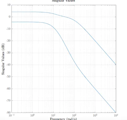
You have forgot your PC and you don’t know the transfer function of the system. Before coming to school, however, you have saved the Matlab plot of the singular values of the system on your phone (see Figure 3. Choose all the possible responses of the system.

Figure 3: Singular values behaviour.

y∞(t) =





0.5·sin(30·t+ 0.314) 0.5·cos(30·t) 0.5·cos(30·t+ 1)





y∞(t) =





4·sin(30·t+ 0.314) 3·cos(30·t) 2·cos(30·t+ 1)





y∞(t) =





0.1·sin(30·t+ 0.314) 0.1·cos(30·t) 0.1·cos(30·t+ 1)





y∞(t) =





0 4·cos(30·t) 2·cos(30·t+ 1)





2·cos(30·t+ 0.243)

Solution.

3





0.5·sin(30·t+ 0.314) 0.5·cos(30·t) 0.5·cos(30·t+ 1)





y_∞(t) =





4·sin(30·t+ 0.314) 3·cos(30·t) 2·cos(30·t+ 1)





y∞(t) =





0.1·sin(30·t+ 0.314) 0.1·cos(30·t) 0.1·cos(30·t+ 1)





3





0 4·cos(30·t) 2·cos(30·t+ 1)





3





2·cos(30·t+ 0.243) 2·cos(30·t+ 0.142) 2·cos(30·t+ 0.252)





Explanation

From the given input one can read

||µ||=√

3² + 4² = 5.

From the plot one can read at ω = 30^rad_s σ_min = 0.1 and σ_max = 1. It follows 5·σmin = 0.5≤ ||ν|| ≤5 = 5·σmax.

The first response has ||ν||=√

0.75 that is in the range. The second response has ||ν||=√ 29 that is too big to be in the range. The third response has ||ν|| =√

0.03 that is to small to be in the range. The fourth response has ||ν||=√

20 that is in the range. The fifth response has

||ν||=√

12 that is in the range.