LAMBDA CALCULI WITH TYPES Henk Barendregt
Catholic University Nijmegen
To appear in
Handbook of Logic in Computer Science, Volume II, Edited by
S. Abramsky, D.M. Gabbay and T.S.E. Maibaum Oxford University Press
Comments are welcome. Author's address:
Faculty of Mathematics and Computer Science Toernooiveld 1
6525 ED Nijmegen The Netherlands E-mail: henk@cs.kun.nl
Lambda Calculi with Types
H.P. Barendregt
Contents
1 Introduction : : : : : : : : : : : : : : : : : : : : : : : : : : : : : : 4 2 Type-free lambda calculus : : : : : : : : : : : : : : : : : : : : : : 7 2.1 The system : : : : : : : : : : : : : : : : : : : : : : : : : : : 7 2.2 Lambda denability : : : : : : : : : : : : : : : : : : : : : : 14 2.3 Reduction : : : : : : : : : : : : : : : : : : : : : : : : : : : : 20 3 Curry versus Church typing : : : : : : : : : : : : : : : : : : : : : 34 3.1 The system !-Curry : : : : : : : : : : : : : : : : : : : : : 34 3.2 The system !-Church : : : : : : : : : : : : : : : : : : : : 42 4 Typinga la Curry : : : : : : : : : : : : : : : : : : : : : : : : : : 46 4.1 The systems : : : : : : : : : : : : : : : : : : : : : : : : : : : 47 4.2 Subject reduction and conversion : : : : : : : : : : : : : : : 57 4.3 Strong normalization : : : : : : : : : : : : : : : : : : : : : : 61 4.4 Decidability of type assignment : : : : : : : : : : : : : : : : 67 5 Typinga la Church : : : : : : : : : : : : : : : : : : : : : : : : : 76 5.1 The cube of typed lambda calculi : : : : : : : : : : : : : : : 77 5.2 Pure type systems : : : : : : : : : : : : : : : : : : : : : : : 96 5.3 Strong normalization for the -cube : : : : : : : : : : : : : 114 5.4 Representing logics and data-types : : : : : : : : : : : : : : 132 5.5 Pure type systems not satisfying normalization : : : : : : : 163 References : : : : : : : : : : : : : : : : : : : : : : : : : : : : : : : : : 184
1
Dedication
This work is dedicated to
Nol andRiet Prager
the musician/philosopher and the poet.
Acknowledgements
Two persons have been quite inuential on the form and contents of this chapter. First of all, Mariangiola Dezani-Ciancaglini claried to me the essential dierences between the Curry and the Church typing systems.
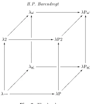
She provided a wealth of information on these systems (not all of which has been incorporated in this chapter; see the forthcoming Barendregt and Dekkers (to appear) for more on the subject). Secondly, Bert van Benthem Jutting introduced me to the notion of type dependency as presented in the systems AUTOMATH and related calculi like the calculus of construc- tions. His intimate knowledge of these calculi|obtained after extensive mathematical texts in them|has been rather useful. In fact it helped me to introduce a ne structure of the calculus of constructions, the so called -cube. Contributions of other individuals|often important ones|will be clear form the contents of this chapter.
The following persons gave interesting input or feedback for the con- tents of this chapter: Steen van Bakel, Erik Barendsen, Stefano Berardi, Val Breazu-Tannen, Dick (N.G.) de Bruijn, Adriana Compagnoni, Mario Coppo, Thierry Coquand, Wil Dekkers, Ken-etsu Fujita, Herman Geu- vers, Jean-Yves Girard, Susumu Hayashi, Leen Helmink, Kees Hemerik, Roger Hindley, Furio Honsell, Martin Hyland, Johan de Iongh, Bart Jacobs, Hidetaka Kondoh, Giuseppe Longo, Sophie Malecki, Gregory Mints, Al- bert Meyer, Reinhard Muskens, Mark-Jan Nederhof, Rob Nederpelt, Andy Pitts, Randy Pollack, Andre Scedrov, Richard Statman, Marco Swaen, Jan Terlouw, Hans Tonino, Yoshihito Toyama, Anne Troelstra and Roel de Vri- jer.Financial support came from several sources. First of allOxford Uni- versity Press gave the necessary momentum to write this chapter. The Research Institute for Declarative Systems at theDepartment of Computer Science of the Catholic University Nijmegen provided the daily environ- ment where I had many discussions with my colleagues and Ph.D. stu- dents. The EC Stimulation Project ST2J-0374-C (EDB)lambda calcul type
helped me to meet many of the persons mentioned above, notably Berardi and Dezani-Ciancaglini. Nippon Telephon and Telegraph (NTT) made it possible to meet Fujita and Toyama. The most essential support came from Philips Research Laboratories Eindhoven where I had extensive discussions with van Benthem Jutting leading to the denition of the -cube.
Finally I would thank Marielle van der Zandt and Jane Spurr for typing and editing the never ending manuscript and Wil Dekkers for proofreading and suggesting improvements. Erik Barendsen was my guru for TEX. Use has been made of the macros of Paul Taylor for commutative diagrams and prooftrees. Erik Barendsen, Wil Dekkers and Herman Geuvers helped me with the production of the nal manuscript.
Nijmegen, December 20, 1991 Henk Barendregt
1 Introduction
The lambda calculus was originally conceived by Church (1932;1933) as part of a general theory of functions and logic, intended as a foundation for mathematics. Although the full system turned out to be inconsistent, as shown in Kleene and Rosser(1936), the subsystem dealing with func- tions only became a successful model for the computable functions. This system is called now the lambda calculus. Books on this subject e.g. are Church(1941), Curry and Feys (1988), Curryet al.(1958; 1972), Barendregt [1984), Hindley and Seldin(1986) and Krivine(1990).
In Kleene and Rosser (1936) it is proved that all recursive functions can be represented in the lambda calculus. On the other hand, in Turing(1937) it is shown that exactly the functions computable by a Turing machine can be represented in the lambda calculus. Representing computable functions as -terms, i.e. as expressions in the lambda calculus, gives rise to so-called functional programming. See Barendregt(1990) for an introduction and references.
The lambda calculus, as treated in the references cited above, is usu- ally referred to as atype-freetheory. This is so, because every expression (considered as a function) may be applied to every other expression (con- sidered as an argument). For example, the identity functionI= x:x may be applied to any argument x to give as result that same x. In particular
Imay be applied to itself.
There are also typed versions of the lambda calculus. These are intro- duced essentially in Curry (1934) (for the so-called combinatory logic, a
variant of the lambda calculus) and in Church (1940). Types are usually objects of a syntactic nature and may be assigned to lambda terms. If M is such a term and, a type A is assigned to M, then we say `M has type A' or `M inA'; the notation used for this is M : A. For example in most systems with types one has I : (A!A), that is, the identityI may get as type A!A. This means that if x being an argument ofIis of type A, then also the value Ix is of type A. In general A!B is the type of functions from A to B.
Although the analogy is not perfect, the type assigned to a term may be compared to the dimension of a physical entity. These dimensions prevent us from wrong operations like adding 3 volts to 2 amperes. In a similar way types assigned to lambda terms provide a partial specication of the algorithms that are represented and are useful for showing partial correct- ness.
Types may also be used to improve the eciency of compilation of terms representing functional algorithms. If for example it is known (by looking at types) that a subexpression of a term (representing a functional program) is purely arithmetical, then fast evaluation is possible. This is because the expression then can be executed by the ALU of the machine and not in the slower way in which symbolic expressions are evaluated in general.
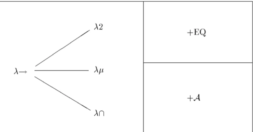
The two original papers of Curry and Church introducing typed versions of the lambda calculus give rise to two dierent families of systems. In the typed lambda calculi a la Curry terms are those of the type-free theory.
Each term has a set of possible types. This set may be empty, be a singleton or consist of several (possibly innitely many) elements. In the systems a la Church the terms are annotated versions of the type-free terms. Each term has a type that is usually unique (up to an equivalence relation) and that is derivable from the way the term is annotated.
The Curry and Church approaches to typed lambda calculus correspond to two paradigms in programming. In the rst of these a program may be written without typing at all. Then a compiler should check whether a type can be assigned to the program. This will be the case if the program is correct. A well-known example of such a language is ML, see Milner (1984). The style of typing is called `implicit typing'. The other paradigm in programming is called `explicit typing' and corresponds to the Church version of typed lambda calculi. Here a program should be written together with its type. For these languages type-checking is usually easier, since no types have to be constructed. Examples of such languages are ALGOL 68 and PASCAL. Some authors designate the Curry systems as `lambda calculiwith type assignment' and the Church systems as `systems oftyped lambda calculus'.
Within each of the two paradigms there are several versions of typed lambda calculus. In many important systems, especially thosea la Church,
it is the case that terms that do have a type always possess a normal form. By the unsolvability of the halting problem this implies that not all computable functions can be represented by a typed term, see Barendregt (1990), theorem 4.2.15. This is not so bad as it sounds, because in order to nd such computable functions that cannot be represented, one has to stand on one's head. For example in 2, the second-order typed lambda calculus, only those partial recursive functions cannot be represented that happen to be total, but not provably so in mathematical analysis (second- order arithmetic).
Considering terms and types as programs and their specications is not the only possibility. A type A can also be viewed as a proposition and a term M in A as a proof of this proposition. This so-called propositions-as- types interpretation is independently due to de Bruijn (1970) and Howard (1980) (both papers were conceived in 1968). Hints in this direction were given in Curry and Feys (1958) and in Lauchli (1970). Several systems of proof checking are based on this interpretation of propositions-as-types and of proofs-as-terms. See e.g. de Bruijn (1980) for a survey of the so-called AUTOMATH proof checking system. Normalization of terms corresponds in the formulas-as-types interpretation to normalisation of proofs in the sense of Prawitz (1965). Normal proofs often give useful proof theoretic information, see e.g. Schwichtenberg (1977). In this chapter several typed lambda calculi will be introduced, botha la Curry anda la Church. Since in the last two decades several dozens of systems have appeared, we will make a selection guided by the following methodology.
Only the simplest versions of a system will be consid- ered. That is, only with -reduction, but not with e.g.
-reduction. The Church systems will have types built up using only ! and , not using e.g. or . The Curry systems will have types built up using only!,\and .
(For this reason we will not consider systems of constructive type theory as developed e.g. in Martin-Lof (1984), since in these theories plays an essential role.) It will be seen that there are already many interesting systems in this simple form. Understanding these will be helpful for the understanding of more complicated systems. No semantics of the typed lambda calculi will be given in this chapter. The reason is that, especially for the Church systems, the notion of model is still subject to intensive investigation. Lambek and Scott (1986) and Mitchell (1990), a chapter on typed lambda calculus in another handbook, do treat semantics but only for one of the systems given in the present chapter. For the Church systems several proposals for notions of semantics have been proposed.
These have been neatly unied using bred categories in Jacobs (1991). See
also Pavlovic (1990). For the semantics of the Curry systems see Hindley (1982), (1983) and Coppo (1985). A later volume of this handbook will contain a chapter on the semantics of typed lambda calculi.
Barendregt and Hemerik (1990) and Barendregt (1991) are introductory versions of this chapter. Books including material on typed lambdacalculus are Girardet al. (1989) (treats among other things semantics of the Church version of 2), Hindley and Seldin (1986) (Curry and Church versions of !), Krivine (1990) (Curry versions of 2 and \), Lambek and Scott (1986) (categorical semantics of !) and the forthcoming Barendregt and Dekkers (199-) and Nerode and Odifreddi (199-).
Section 2 of this chapter is an introduction to type-free lambda-calculus and may be skipped if the reader is familiar with this subject. Section 3 explains in more detail the Curry and Church approach to lambda calculi with types. Section 4 is about the Curry systems and Section 5 is about the Church systems. These two sections can be read independently of each other.
2 Type-free lambda calculus
The introduction of the type-free lambda calculus is necessary in order to dene the system of Curry type assignment on top of it. Moreover, al- though the Church style typed lambda calculi can be introduced directly, it is nevertheless useful to have some knowledge of the type-free lambda calculus. Therefore this section is devoted to this theory. For more infor- mation see Hindley and Seldin [1986] or Barendregt [1984].
2.1 The system
In this chapter the type-free lambda calculus will be called `-calculus' or simply . We start with an informal description.
Application and abstraction
The -calculus has two basic operations. The rst one is application. The expression
F:A
(usually written as FA) denotes the data F considered as algorithm applied to A considered as input. The theory istype-free: it is allowed to consider expressions like FF, that is, F applied to itself. This will be useful to simulate recursion.
The other basic operation isabstraction. If M M[x] is an expression containing (`depending on') x, then x:M[x] denotes the intuitive map
x7!M[x];
i.e. to x one assigns M[x]. The variable x does not need to occur actually in M. In that case x:M[x] is a constant function with value M.
Application and abstraction work together in the following intuitive formula:
(x:x2+ 1)3 = 32+ 1 (= 10):
That is, (x:x2+ 1)3 denotes the function x 7! x2+ 1 applied to the argument 3 giving 32+ 1 (which is 10). In general we have
(x:M[x])N = M[N]:
This last equation is preferably written as
(x:M)N = M[x := N]; ()
where [x := N] denotes substitution of N for x. This equation is called -conversion. It is remarkable that although it is the only essential axiom of the -calculus, the resulting theory is rather involved.
Free and bound variables
Abstraction is said to bindthefree variable x in M. For example, we say that x:yx has x as bound and y as free variable. Substitution [x := N] is only performed in the free occurrences of x:
yx(x:x)[x := N] = yN(x:x):
In integral calculus there is a similar variable binding. InRabf(x;y)dx the variable x is bound and y is free. It does not make sense to substitute 7 for x, obtainingRbaf(7;y)d7; but substitution for y does make sense, obtaining
Ra
b f(x;7)dx.
For reasons of hygiene it will always be assumed that the bound vari- ables that occur in a certain expression are dierent from the free ones.
This can be fullled by renaming bound variables. For example, x:x be- comes y:y. Indeed, these expressions act the same way:
(x:x)a = a = (y:y)a
and in fact they denote the same intended algorithm. Therefore expressions that dier only in the names of bound variables are identied. Equations like x:xy:y are usually called -conversion.
Functions of several arguments
Functions of several arguments can be obtained by iteration of application.
The idea is due to Schonnkel (1924) but is often called `currying', after H.B. Curry who introduced it independently. Intuitively, if f(x;y) depends on two arguments, one can dene
Fx = y:f(x;y) F = x:Fx:
Then (Fx)y = Fxy = f(x;y): (1)
This last equation shows that it is convenient to useassociation to the left for iterated application:
FM1:::Mndenotes (::((FM1)M2):::Mn):
The equation (1) then becomes
Fxy = f(x;y):
Dually, iterated abstraction uses association to the right:
x1xn:f(x1;:::;xn) denotes x1:(x2:(:::(xn:f(x1;:::;xn))::)):
Then we have for F dened above
F = xy:f(x;y) and (1) becomes
(xy:f(x;y))xy = f(x;y):
For n arguments we have
(x1:::xn:f(x1;:::;xn))x1:::xn= f(x1;:::;xn);
by using () n times. This last equation becomes in convenient vector notation
(~x:f(~x))~x = f(~x);
more generally one has
(~x:f(~x)) ~N = f( ~N):
Now we give the formal description of the -calculus.
Denition 2.1.1. The set of -terms, notation , is built up from an innite set of variables V =fv;v0;v00;:::gusing application and (function) abstraction:
x2V ) x2;
M;N2 ) (MN)2;
M 2;x2V ) (xM)2: Using abstract syntax one may write the following.
V ::= vjV0
::= V j()j(V ) Example 2.1.2. The following are -terms:
v;(vv00);
(v(vv00));
((v(vv00))v0);
((v0((v(vv00))v0))v000):
Convention 2.1.3.
1. x;y;z;::: denote arbitrary variables;
M;N;L;::: denote arbitrary -terms.
2. As already mentioned informally,the followingabbreviations are used:
FM1:::Mn stands for (::((FM1)M2):::Mn) and x1xn:M stands for (x1(x2(:::(xn(M))::))):
3. Outermost parentheses are not written.
Using this convention, the examples in 2.1.2 now may be written as follows:
x;xz;x:xz;
(x:xz)y;
(y:(x:xz)y)w:
Note that x:yx is (x(yx)) and not ((xy)x).
Notation 2.1.4. M N denotes that M and N are the same term or can be obtained from each other by renaming bound variables. For example,
(x:x)z (x:x)z;
(x:x)z (y:y)z;
(x:x)z 6 (x:y)z:
Denition 2.1.5.
1. The set of free variablesof M, (notation FV (M)), is dened induc- tively as follows:
FV (x) = fxg;
FV (MN) = FV (M)[FV (N);
FV (x:M) = FV (M) fxg:
2. M is a closed -term (or combinator) if FV (M) = ;. The set of closed -terms is denoted by 0.
3. The result ofsubstitution of N for (the free occurrences of) x in M, notation M[x := N], is dened as follows: Below x6y.
x[x := N] N;
y[x := N] y;
(PQ)[x := N] (P[x := N])(Q[x := N]);
(y:P)[x := N] y:(P[x := N]); provided y6x;
(x:P)[x := N] (x:P):
In the -term
y(xy:xyz)
y and z occur as free variables; x and y occur as bound variables. The term xy:xxy is closed.
Names of bound variables will be always chosen such that they dier from the free ones in a term. So one writes y(xy0:xy0z) for y(xy:xyz).
This so-called `variable convention' makes it possible to use substitution for the -calculus without a proviso on free and bound variables.
Proposition 2.1.6 (Substitution lemma). Let M;N;L2. Suppose x6y and x =2FV (L). Then
M[x := N][y := L]M[y := L][x := N[y := L]]:
Proof. By induction on the structure of M.
Now we introduce the -calculus as a formaltheory of equations between -terms.
Denition 2.1.7.
1. The principal axiom scheme of the -calculus is
(x:M)N = M[x := N] ()
for all M;N 2. This is called -conversion. 2. There are also the `logical' axioms and rules:
M = M;
M = N ) N = M;
M = N;N = L ) M = L;
M = M0 ) MZ = M0Z;
M = M0 ) ZM = ZM0;
M = M0 ) x:M = x:M0: ()
3. If M = N is provable in the -calculus, then we write `M = N or sometimes just M = N.
Remarks 2.1.8.
1. We have identied terms that dier only in the names of bound vari- ables. An alternative is to add to the -calculus the following axiom scheme of -conversion.
x:M = y:M[x := y]; ()
provided that y does not occur in M. The axiom () above was originally the second axiom; hence its name. We prefer our version of the theory in which the identications are made on a syntactic level.
These identications are done in our mind and not on paper.
2. Even if initially terms are written according to the variable conven- tion, -conversion (or its alternative) is necessary when rewriting terms. Consider e.g. !x:xx and 1yz:yz. Then
!1 (x:xx)(yz:yz)
= (yz:yz)(yz:yz)
= z:(yz:yz)z
z:(yz0:yz0)z
= zz0:zz0
yz:yz
1:
3. For implementations of the -calculus the machine has to deal with this so called -conversion. A good way of doing this is provided by the `name-free notation' of N.G. de Bruijn, see Barendregt (1984), Appendix C. In this notation x(y:xy) is denoted by (21), the 2 denoting a variable bound `two lambdas above'.
The following result provides one way to represent recursion in the - calculus.
Theorem 2.1.9 (Fixed point theorem).
1. 8F9XFX = X:
(This means that for all F2 there is an X2 such that `FX = X:) 2. There is a xed point combinator
Yf:(x:f(xx))(x:f(xx)) such that
8F F(YF) =YF:
Proof. 1. Dene W x:F(xx) and XWW. Then X WW (x:F(xx))W = F(WW)FX:
2. By the proof of (1). Note that
YF = (x:F(xx))(x:F(xx))X:
Corollary 2.1.10. Given a term CC[f;x] possibly containing the dis- played free variables, then
9F8X FX = C[F;X]:
Here C[F;X] is of course the substitution result C[f := F][x := X]:
Proof. Indeed, we can construct F by supposing it has the required prop- erty and calculating back:
8X FX = C[F;X]
( Fx = C[F;x]
( F = x:C[F;x]
( F = (fx:C[f;x])F
( F Y(fx:C[f;x]):
This also holds for more arguments: 9F8~x F~x = C[F;~x]:
As an application, terms F and G can be constructed such that for all terms X and Y
FX = XF;
GXY = Y G(Y XG):
2.2 Lambda denability
In the lambda calculus one can dene numerals and represent numeric functions on them.
Denition 2.2.1.
1. Fn(M) with n2N(the set of natural numbers) and F;M 2, is dened inductively as follows:
F0(M) M;
Fn+1(M) F(Fn(M)):
2. TheChurch numeralsc0;c1;c2;::: are dened by cnfx:fn(x):
Proposition 2.2.2 (J. B. Rosser). Dene
A
+
xypq:xp(ypq);
A
xyz:x(yz);
Aexp xy:yx:
Then one has for all n;m2N 1. A+cncm=cn+m:
2. Acncm=cn:m:
3. Aexpcncm =c(nm); except for m = 0 (Rosser starts at 1).
Proof. We need the following lemma.
Lemma 2.2.3.
1. (cnx)m(y) = xnm(y);
2. (cn)m(x) =c(nm)(x); form > 0.
Proof. 1. By induction on m. If m = 0, then LHS = y = RHS. Assume (1) is correct for m (Induction Hypothesis: IH). Then
(cnx)m+1(y) = cnx((cnx)m(y))
=IH cnx(xnm(y))
= xn(xnm(y))
xn+nm(y)
xn(m+1)(y):
2. By induction on m > 0. If m = 1, then LHS cnxRHS. If (2) is correct for m, then
cmn+1(x) = cn(cmn(x))
=IH cn(c(nm)(x))
= y:(c(nm)(x))n(y)
=(1) y:xnmn(y)
= c(nm+1)x:
Now the proof of the proposition.
1. By induction on m.
2. Use the lemma (1).
3. By the lemma (2) we have for m > 0
Aexpcncm =cmcn= x:cnm(x) = x:c(nm)x =c(nm); since x:Mx = M if M = y:M0[y] and x =2FV (M). Indeed,
x:Mx = x:(y:M0[y])x
= x:M0[x]
y:M0[y]
= M:
We have seen that the functions plus, times and exponentiation onN can be represented in the -calculus using Church's numerals. We will show that all computable (recursive) functions can be represented.
Boolean truth values and a conditional can be represented in the - calculus.
Denition 2.2.4 (Booleans, conditional).
1. truexy:x;falsexy:y:
2. If B is a Boolean, i.e. a term that is eithertrue, orfalse, then ifB thenP elseQ
can be represented by BPQ. Indeed, truePQ = P andfalsePQ = Q.
Denition 2.2.5 (Pairing). For M;N 2 write [M;N]z:zMN:
Then [M;N]true= M
[M;N]false= N and hence [M;N] can serve as an ordered pair.
Denition 2.2.6.
1. A numeric function is a map f :Np!Nfor some p.
2. A numeric function f with p arguments is called -denable if one has for some combinator F
Fcn1:::cnp =cf(n1;:::;np) (1) for all n1;:::;np2N. If (1) holds, then f is said to be -dened by F.
Denition 2.2.7.
1. Theinitial functions are the numeric functions Uir;S+;Z dened by:
Uir(x1;:::;xr) = xi; 1ir;
S+(n) = n + 1;
Z(n) = 0:
2. Let P(n) be a numeric relation. As usual m:P(m)
denotes the least number m such that P(m) holds if there is such a number; otherwise it is undened.
As we know from Chapter 2 in this handbook, the class R of recur- sive functions is the smallest class of numeric functions that contains all
initial functions and is closed under composition, primitive recursion and minimalization. SoRis an inductively dened class. The proof that all re- cursive functions are -denable is by a corresponding induction argument.
The result is originally due to Kleene (1936).
Lemma 2.2.8. The initial functions are -denable.
Proof. Take as dening terms
Uip x1xp:xi;
S +
xyz:y(xyz) (=A+c1);
Z x:c0:
Lemma 2.2.9. The -denable functions are closed under composition.
Proof. Let g;h1;:::;hmbe -dened by G;H1;:::;Hmrespectively. Then f(~n) = g(h1(~n);:::;hm(~n))
is -dened by
F ~x:G(H1~x):::(Hm~x):
Lemma 2.2.10. The-denable functions are closed under primitive re- cursion.
Proof. Let f be dened by
f(0;~n) = g(~n)
f(k + 1;~n) = h(f(k;~n);k;~n)
where g;h are -dened by G;H respectively. We have to show that f is - denable. For notational simplicity we assume that there are no parameters
~n (hence G =cf(0).) The proof for general ~n is similar.
If k is not an argument of h, then we have the scheme of iteration.
Iteration can be represented easily in the -calculus, because the Church numerals are iterators. The construction of the representation of f is done
in two steps. First primitive recursion is reduced to iteration using ordered pairs; then iteration is represented. Here are the details. Consider
T p:[S+(ptrue);H(pfalse)(ptrue)]:
Then for all k one has
T([ck;cf(k)]) = [fS+ck;Hcf(k)ck]
= [ck+1;cf(k+1)]:
By induction on k it follows that
[ck;cf(k)] = Tk[c0;cf(0)]:
Therefore
cf(k)=ckT[c0;cf(0)]false; and f can be -dened by
F k:kT[c0;G]false:
Lemma 2.2.11. The -denable functions are closed under minimaliza- tion.
Proof. Let f be dened by f(~n) = m[g(~n;m) = 0], where ~n = n1;:::;nk
and g is -dened by G. We have to show that f is -denable. Dene zeron:n(true false)true:
Then zero c0 = true,
zero cn+1 = false.
By Corollary 2.1.10 there is a term H such that
H~ny = if (zero(G~ny))theny elseH~n(S+y):
Set F = ~n:H~xc0. Then F -denes f:
Fc~x = Hc~nc0
= c0; if Gc~nc0=c0;
= Hc~nc1 else;
= c1; if Gc~nc1=c0;
= Hc~nc2 else;
= c2; if :::
= :::
Herec~nstands forcn1:::cnk:
Theorem 2.2.12. All recursive functions are-denable.
Proof. By 2.2.8-2.2.11.
The converse also holds. The idea is that if a function is -denable, then its graph is recursively enumerable because equations derivable in the -calculus can be enumerated. It then follows that the function is recur- sive. So for numeric functions we have f is recursive i f is -denable.
Moreover also for partial functions a notion of -denability exists and one has is partial recursive i is -denable. The notions -denable and recursive both are intended to be formalizations of the intuitive concept of computability. Another formalization was proposed by Turing in the form of Turing computable. The equivalence of the notions recursive, -denable and Turing computable (for the latter see besides the original Turing, 1937, e.g., Davis 1958) Davis provides some evidence for the Church{Turing the- sis that states that `recursive' is the proper formalization of the intuitive notion `computable'.
We end this subsection with some undecidability results. First we need the coding of -terms. Remember that the collection of variables isfv;v0;v00;:::g.
Denition 2.2.13.
1. Notation. v(0) = v; v(n+1)= v(n)0.
2. Leth; ibe a recursive coding of pairs of natural numbers as a natural number. Dene
](v(n)) = h0;ni;
](MN) = h2;h](M);](N)ii; ](x:M) = h3;h](x);](M)ii: 3. Notation
pMq=c]M: Denition 2.2.14. LetA.
1. A is closed under = if
M 2A; `M = N ) N2A: 2. A is non-trivial ifA6=;andA6= :
3. A is recursiveif ]A=f]M jM 2Agis recursive.
The following result due to Scott is quite useful for proving undecidability results.
Theorem 2.2.15. LetA be non-trivial and closed under=. ThenA is not recursive.
Proof. (J. Terlouw) Dene
B=fM jMpMq2Ag:
Suppose A is recursive; then by the eectiveness of the coding also B is recursive (indeed, n2]B,h2;hn;]cnii2]A). It follows that there is an F20with
M2B , FpMq=c0; M =2B , FpMq=c1: Let M02A;M12=A. We can nd a G2 such that
M2B , GpMq= M12=A; M =2B , GpMq= M02A:
[Take Gx =if zero(Fx)thenM1elseM0, withzerodened in the proof of 2.2.11.] In particular
G2B , GpGq2=A ,Def G =2B; G =2B , GpGq2A ,Def G2B; a contradiction.
The following application shows that the lambda calculus is not a de- cidable theory.
Corollary 2.2.16 (Church). The set
fM jM = trueg is not recursive.
Proof. Note that the set is closed under = and is nontrivial.
2.3 Reduction
There is a certain asymmetry in the basic scheme (). The statement (x:x2+ 1)3 = 10
can be interpreted as `10 is the result of computing (x:x2+ 1)3', but not vice versa. This computational aspect will be expressed by writing
(x:x2+ 1)3 !! 10 which reads `(x:x2+ 1)3reduces to 10'.
Apart from this conceptual aspect, reduction is also useful for an ana- lysis of convertibility. The Church{Rosser theorem says that if two terms are convertible, then there is a term to which they both reduce. In many cases the inconvertibility of two terms can be proved by showing that they do not reduce to a common term.
Denition 2.3.1.
1. A binary relation R on is calledcompatible (w.r.t. operations) if M R N ) (ZM) R (ZN);
(MZ) R (NZ), and (x:M) R (x:N):
2. A congruence relation on is a compatible equivalence relation.
3. A reduction relation on is a compatible, reexive and transitive relation.
Denition 2.3.2. The binary relations!,!! and = on are dened inductively as follows:
1. (a) (x:M)N !M[x := N];
(b) M ! N ) ZM! ZN; MZ!NZ and x:M !x:N:
2. (a) M !!M;
(b) M ! N ) M !!N;
(c) M !!N;N !!L ) M !!L.
3. (a) M !!N ) M =N;
(b) M =N ) N =M;
(c) M =N;N = L ) M = L:
These relations are pronounced as follows:
M !!N : M -reduces toN;
M !N : M -reduces toN in one step; M =N : M is -convertible toN:
By denition! is compatible. The relation!!is the reexive transitive closure of ! and therefore a reduction relation. The relation = is a congruence relation.
Proposition 2.3.3. M =N , `M = N:
Proof. (() By induction on the generation of`. ()) By induction one shows
M !N ) `M = N;
M !!N ) `M = N;
M = N ) `M = N:
Denition 2.3.4.
1. A -redex is a term of the form (x:M)N. In this case M[x := N] is itscontractum.
2. A -term M isa -normal form(-nf) if it does not have a -redex as subexpression.
3. A term M hasa -normal form if M =N and N is a -nf, for some N.
Example 2.3.5. (x:xx)y is not a -nf, but has as -nf the term yy.
An immediate property of nf's is the following.
Lemma 2.3.6. Let M;M0;N;L2. 1. Suppose M is a -nf. Then
M !! N ) N M:
2. If M ! M0, then M[x := N]!M0[x := N].
Proof. 1. If M is a -nf, then M does not contain a redex. Hence never M !N. Therefore if M!!N, then this must be because M N.
2. By induction on the generation of!.
Theorem 2.3.7 (Church{Rosser theorem). If M !!N1;M !!N2, then for some N3 one has N1!! N3 and N2!!N3; in diagram
M
@
@
@
@ R
N1 RN2
...
...RR ............
N3 The proof is postponed until 2.3.17.
Corollary 2.3.8. If M =N, then there is an L such that M !!L and N !!L.
Proof. Induction on the generation of =.
Case 1. M =N because M !!N. Take LN.
Case 2. M = N because N = M. By the IH there is a common -reduct L1 of N;M: Take LL1.
Case 3. M =N because M =N0;N0=N. Then
M (IH) N0 (IH) N
@
@
@
@ R
R
@
@
@
@ R
L1 CR RL2
...RR... ..........
L Corollary 2.3.9.
1. If M has N as -nf, then M !!N.
2. A -term has at most one -nf.