LIST OF FIGURES AND TABLES

(1)

DISSERTATION

submitted to the

Combined Faculties for Natural Sciences and Mathematics of the Ruperto – Carola University of Heidelberg, Germany

for the degree of Doctor of Natural Sciences

presented by Reinhold Josef Dorn

born in Munich

Oral examination: 21. November 2001

(2)

(3)

A CCD BASED CURVATURE WAVEFRONT SENSOR FOR ADAPTIVE OPTICS IN ASTRONOMY

Referees: Professor Dr. Immo Appenzeller Professor Dr. Josef Bille

(4)

(5)

ZUSAMMENFASSUNG

Adaptive Optik (AO) ist eine Technik, um Störungen in der Abbildung von Objekten im Teleskop auszugleichen. Diese Störungen werden von Fluktuationen des Brechungsindexes in der Erdatmosphäre hervorgerufen. Zum Messen dieser Störungen gibt es eine Reihe verschiedener Wellenfrontsensoren. Einer davon ist der “Curvature”- Wellenfrontsensor, was soviel wie “Krümmungs”- Wellenfrontsensor bedeutet. An der Europäischen Südsternwarte (ESO) in Garching werden für das Very Large Telescope (VLT) und das VLT Interferometer (VLTI) eine Reihe von adaptiven Optiksystemen entwickelt, die den Curvature - Wellenfrontsensor verwenden. Bisher wurden in Curvature AO-Systemen Avalanche Photodioden (APDs) als Detektoren verwendet, da sehr kurze Belichtungszeiten (200 Mikrosekunden) und ein sehr niedriges Ausleserauschen des Detektors nötig sind.

Aufgrund von Fortschritten in der Herstellungstechnologie von Charge Coupled Devices (CCDs) entwickelten wir ein spezielles CCD und untersuchten dessen Leistungsfähigkeit für ein 60 Element Curvature AO System, das mit sehr schwachen Lichtsignalen arbeitet. Hier wurde erstmals ein CCD als Wellenfrontsensor verwendet. Diese Dissertation zeigt, daß ein CCD annäherend die gleiche Leistungsfähigkeit wie APDs bietet, jedoch zu einem Bruchteil der Kosten und geringerer Komplexität. Weiter hat das CCD eine höhere Quantenausbeute und einen größeren dynamischen Bereich als APDs. Ein Ausleserauschen von weniger als 1,5 Elektronen bei 4000 Bildern pro Sekunde wurde erreicht. Für AO Systeme, die Wellenfrontkorrekturen mit vielen Elementen durchführen, können dünne, von hinten beleuchtete CCDs, APDs als bessere Detektoren ersetzen.

Diese Dissertation präsentiert das Konzept, das Design und die Bestimmung der Leistungsfähigkeit dieses CCDs. Erste (von vorne beleuchtete) CCDs wurden erfolgreich getestet und die Leistungsfähigkeit in einem Laborexperiment nachgewiesen.

ABSTRACT

Adaptive Optics (AO) is a technique for compensating the distortions introduced by atmospheric turbulence in astronomical imaging. To measure the distortions a wavefront sensor is needed. There are a number of fundamentally different types of wavefront sensors, one of which is the curvature wavefront sensor. At the European Southern Observatory (ESO) in Garching, Germany, several adaptive optics systems using curvature wavefront sensors are being developed for the Very Large Telescope (VLT) and the VLT interferometer (VLTI). Curvature AO-systems have traditionally used avalanche photodiodes (APDs) as detectors due to strict requirements of very short integration times (200 microsec) and very low readout noise.

Advances in charge-coupled device (CCD) technology motivated an investigation of the use of a specially designed CCD as the wavefront sensor detector in a 60-element curvature AO system. A CCD has never been used before as the wavefront sensor in a low light level curvature adaptive optics system. This thesis shows that a CCD can achieve nearly the same performance as APDs at a fraction of the cost and with reduced complexity for high order wavefront correction. Moreover the CCD has higher quantum efficiency and a greater dynamic range than APDs. A readout noise of less than 1.5 electrons at 4000 frames per second was achieved. A back-illuminated thinned version of this CCD can replace APDs as the best detector for high order curvature wavefront sensing.

This thesis presents the concept, the design and the evaluation of the CCD. The first frontside devices were successfully evaluated and the performance of the detector was proven in a laboratory experiment.

(6)

(7)

LIST OF FIGURES AND TABLES

Number Page

Chapter 1

Fig. 1-1 Schematic diagram of an adaptive optics system...2

Chapter 2 Fig. 2-1 Diffraction-limited PSF of an 8 m telescope at a wavelength of 1000 nm with 0.65" seeing ...6

Fig. 2-2 Speckle pattern of an 8 m telescope at a wavelength of 1000 nm with 0.65"seeing...6

Fig. 2-3 Seeing disk (c) of an 8 m telescope at a wavelength of 1000 nm with 0.65" seeing...6

Fig. 2-4 Resolution of a telescope with turbulence...8

Fig. 2-5 Integrated uncorrected PSF with a Strehl ratio of 8% (a), integrated corrected PSF with a Strehl ratio of 49% (b), and diffraction-limited PSF (c)...9

Fig. 2.6 Main types of deformable mirrors used in astronomical adaptive optics...10

Fig. 2-7 Examples of Zernike polynominals...12

Tab. 2-1 Modified Zernike polynomials after Noll and the mean square residual amplitudes for Kolmogorov turbulence after removal of the first j terms. ...11

Chapter 3 Fig. 3-1 Distortion free image...15

Fig. 3-2 A schematic diagram of the principles of Shack-Hartmann...16

Fig. 3-3 EEV CCD-50 used for the NAOS visible wavefront sensor ...17

Fig. 3-4 Spot images of a 14 x 14 lenslet array and computed spot location ...18

Fig. 3-5 Shearing interferometer that uses a diffraction grating ...18

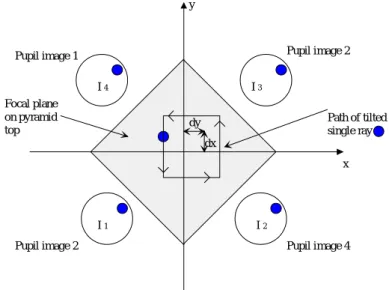
Fig. 3-6 Principle of pyramid wavefront sensing ...19

Fig. 3-7 Pyramid wavefront sensing - principle operation...20

Fig. 3-8 A schematic diagram of the principles of curvature wavefront sensing ...22

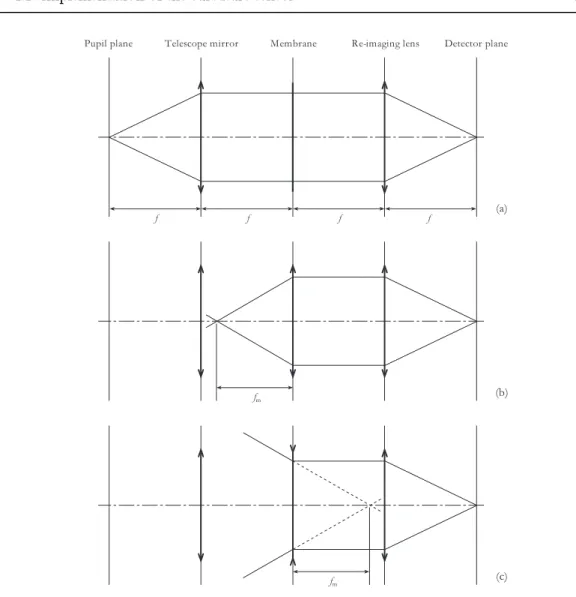
Fig. 3-9 A flat wavefront focused by a lens, showing the intrafocal and extrafocal image planes on either side of the focal plane ...23

Fig. 3-10 Propagation of a flat but tilted wavefront and the resulting curvature signal...25

Fig. 3-11 Computer simulation of curvature wavefront sensing...26

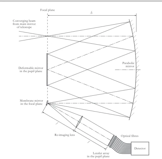
Chapter 4 Fig. 4-1 Schematic diagram of the typical optical layout of a low light level astronomical AO curvature wavefront sensor...28

Fig. 4-2 Geometrical optics analysis of the curvature wavefront sensor...29

Fig. 4-3 Geometry of the membrane mirror in a curvature AO system ...29

(10)

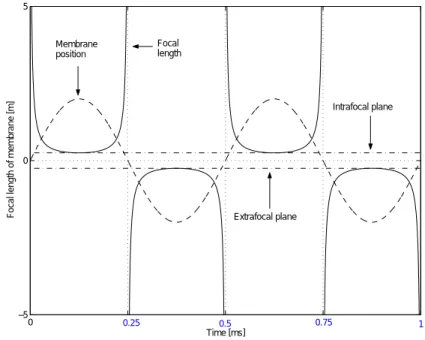
Fig. 4-4 Membrane amplitude and membrane focal length as a function of time...30

Fig. 4-5 Subaperture geometry for ESO's 60 element curvature AO system...32

Fig. 4-6 Division of converging power between two lenslets arrays...32

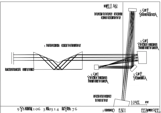
Fig. 4-7 Optical layout of the wavefront sensor box for the MACAO VLTI system...33

Fig. 4-8 Picture of an APD from Perkin Elmer...34

Fig. 4-9 APD quantum efficiency ...34

Fig. 4-10 Instantaneous and integrated Strehl ratios at 2.2 microns when using APDs and 16th magnitude guide star with no separate tip/tilt sensor ...35

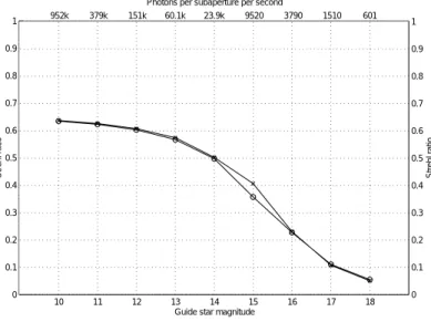
Fig. 4-11 Integrated Strehl as a function of guide star magnitude for APD detectors with and without separate tip/tilt sensor...36

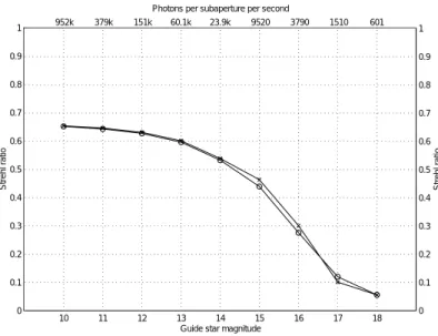
Fig. 4-12 Performance of the APD and CCD without a tip/tilt sensor...37

Fig. 4-13 Performance of the APD and CCD with a tip/tilt sensor that utilizes 20% of the photons ...37

Tab. 4-1 Parameters used in the simulation ...37

Chapter 5 Fig. 5-1 Schematic cross section of a buried channel capacitor ...41

Fig. 5-2 Energy band diagrams for a burried channel CCD - (a) unbiased condition, n-type region is fully depleted, (c) bias voltage applied ...43

Fig. 5-3 Schematic of a single pixel structure...44

Fig. 5-4 Schematic cross section of two cells of a three-phase, n-channel CCD and electron energy at the semiconductor-oxide interface for different applied clock voltages...44

Fig. 5-5 Unit cell overview...45

Fig. 5-6 Superpixel architecture...46

Fig. 5-7 Unit column design - 10 combined unit cells with the output amplifier...47

Fig. 5-8 Unit column design - schematic diagram with the clock phased and output amplifier circuit ...48

Fig. 5-9 Layout of the CCD design for a unit column and the output amplifier design...49

Fig. 5-10 CCD design - curvature wavefront sensor array ...50

Fig. 5-11 Picture of the real device with bonding wires...51

Fig. 5-12 CCID-35 amplifier design...51

Fig. 5-13 MIT/LL wafer layout mask set with the curvature CCDs...53

Fig. 5-14 Frontside and backside illuminated CCDs...53

Fig. 5-15 CCD design - expected quantum efficiency...54

Fig. 5-16 Calculated dark current for the CCID-35 ...55

Fig. 5-17 Picture of the frontside CCID-35, the curvature CCD...56

Fig. 5-18 Example of principle operation...59

Fig. 5-19 Illustration of parallel timing waveforms required for the curvature CCD ...61

Fig. 5-20 Illustration of serial timing waveforms required for the curvature CCD ...62

Fig. 5-21 CCD mode – dark image...63

Fig. 5-22 CCD mode – spot image...63

Fig. 5-23 CCD mode – storage image...64

Fig. 5-24 CCD mode – curvature mode image ...64

Tab. 5-1 Clockphases for the curvature CCD...60

Tab. 5-2 Clockphases for the tracker CCD ...60

Chapter 6 Fig. 6-1 Schematic overview of the Detector system...68

Fig. 6-2 Picture of the prototype laboratory system of the CCD based curvature wavefront sensor ...69

(11)

List of Figures and Tables xi

Fig. 6-3 CCD preamplifier with 4 channels...70

Fig. 6-4 Total transmission efficiency of the fibers used for the curvature sensor as a function of wavelength...71

Fig. 6-5 Support structure of the fibers at the input of the relay optics ...72

Fig. 6-6 Relay optics to be used to reimage the light of the individual fibers onto the CCD ...72

Fig. 6-7 Convex sphere of the Oeffner relay optics during the alignment tests in the laboratory ...73

Fig. 6-8 Spot image of the curvature CCD and horizontal cross section...73

Fig. 6-9 CCD surface analysis...74

Fig. 6-10 CCD cryostat with relay optics...75

Fig. 6-11 CCD cryostat electronics for the CCID-35...76

Fig. 6-12 Diagram from the data sheet of the special LED IPL 10530...77

Fig. 6-13 Lamp circuitry of the stable LED light source...77

Fig. 6-14 Switch-on delay and Switch-off delay of the LED ...78

Fig. 6-15 Schematic diagram of the simulation setup with the integrating sphere and the stable LEDs...79

Fig. 6-16 Picture of the simulation setup for the curvature sensor ...79

Chapter 7 Fig. 7-1 Photon transfer curve; The plot describes three noise regimes of the CCD detector system, 1) read noise 2) shot noise and 3) fixed pattern noise ...82

Fig. 7-2 Example of a “time series” flat field image used for noise calculations with the curvature CCD ...84

Fig. 7-3 Photon transfer curve for the first output amplifier of the CCID-35...85

Fig. 7-4 Determination of the optimal drain voltages for the MOSFET amplifier of the CCID-35 (ID=200 µA)...86

Fig. 7-5 FIERA analog signal chain - schematic overview...87

Fig. 7-6 Linearity curve for the first output amplifier of the CCID-35 with a gain factor of ~0.3 electrons per ADU ...89

Fig. 7-7 Residual non-linearity curve of the first output amplifier of the CCID-35...89

Fig. 7-8 Image of the CCID-35 adding up charge for 100 cycles in the storage pixels SA and SB and a horizontal cross section though storage pixels SA ...90

Fig. 7-9 Clock and bias filter for the fanout printed circuit board inside the cryostat...91

Fig. 7-10 Principle of charge transfer efficiency measurement with the extended pixel edge response method ...92

Fig. 7-11 Pocket pumping response of the CCID-35 for a flat field of 60 electrons per pixels pumped for 1000 cycles. The response shows forward and reverse traps smaller than one electron...94

Fig. 7-12 Horizontal cross section of the vertical line 109 of Figure 7-11 showing a trap located at x-126 and y-109. Also shown a dark pixel at x-61 and y-109 which is proceeding a trap at line 110...95

Fig. 7-13 CCID-35 image with on average 25,000 electrons per pixel in the spots exceeding the full well capacity of the serial register seen as deferred charge trails after bright pixels...97

Fig. 7-14 One hour dark frame of the thick frontside CCID-35 ...98

Fig. 7-15 Measured dark current versus temperature for a single pixel per second and dark current per superpixels (400 pixels) per 20 ms...99

Fig. 7-16 CCD image with ~ 1 electron charge per pixel and a readout noise of 1.4 electrons and a horizontal cross section...100

Fig. 7-17 Average frame of 256 CCD image with ~ 1 electron charge per pixel and a readout noise of ~0.1 electrons and its horizontal cross section...101

(12)

Fig. 7-18 (1) Image adding up intrafocal and extrafocal charge for four cycles, resulting in an image with ~1 electron charge per subaperture. The signal is completely embedded in the noise of the frame. (2) Sum of 16 four-cycle images and (3) sum of 256 four-cycle images added together. For both the 16 image sum and the 256 sum the signal in the individual subapertures is clearly visible. For comparison, the last image (4) shows a frame at much higher signal levels to identify the

subapertures fed with photons via the fibers ... 102

Fig. 7-19 (1) Image adding up only intrafocal charge for four cycles, resulting in an image with ~1 electron charge per subaperture. The signal is completely embedded in the noise of the frame. (2) Sum of 16 four-cycle images and (3) sum of 256 four-cycle images added together. For both the 16 image sum and the 256 sum the signal in the individual subapertures is clearly visible. For comparison, the last image (4) shows a frame at much higher signal levels to identify the subapertures fed with photons via the fibers ...102

Fig. 7-20 Performance of the curvature CCD with 80% quantum efficiency compared to avalanche photodiodes...104

Tab. 7-1 Readout noise results for the CCID-35 with the 20 x 20 binned superpixels in curvature mode. ...85

Tab. 7-2 Residual non-linearity results for the CCID-35 and the corresponding conversion factors ...88

Tab. 7-3 Results of charge transfer efficiency in horizontal and vertical direction at various light levels...93

Tab. 7-4 Specifications of the curvature wavefront sensor detector for APDs and CCDs ...103

Tab. 7-5 Strehl ratios achived with APDs and the curvature CCD with 80% quantum efficiency...103

Tab. 7-6 Loop gains and integration times...104

Appendices Appendix A Picture of the wafer with the curvature CCDs ...109

Appendix B Picture of the CCID-35 die ...110

Appendix C Package layout of the frontside curvature CCD array...111

Appendix D Voltage setting for the clock and bias phases of the frontside CCID-35...112

Appendix E1 Measured linearity curves for the output amplifiers of the curvature CCD ...113

Appendix E2 Measured residual non-linearity curves for the output amplifiers of the curvature CCD...114

Appendix E3 Measured photon transfer curves for the output amplifiers of the curvature CCD ...115

Appendix F Acronyms...116

(13)

ACKNOWLEDGMENTS

The thesis work was carried out as a research and development project within the Instrumentation division at the European Southern Observatory in Garching for future possible wavefront sensors in the growing field of Adaptive Optics. I would like to thank the Instrumentation division management for providing the funds for this project and for giving me the time to finish this thesis despite my new duties in the Infrared Detector Group from June 2000.

Many people have contributed to this work in various ways, some of them I would like to thank here particularly. First of all I would like to thank Dr. James Beletic, my local supervisor and former Head of the Optical Detector and Adaptive Optics groups at ESO, now deputy director of the W. M. Keck Observatory in Hawaii. Despite the physical distance in the last year of the thesis, he never lost oversight of my work and was a great source of knowledge and advice. He made this project possible and I would like to thank him for giving me the confidence and motivation necessary to carry out this research. I greatly appreciate the time he took to carefully proofread the manuscript and the critical comments he made, which improved this thesis in many ways.

Secondly I like to thank Dr. Barry Burke from MIT Lincoln Laboratory for the excellent design of the CCD and for producing it in a very short time frame. Barry Burke has been a great help in making this CCD work. He always took the time to answer my questions in the many e-mails we exchanged.

I greatly appreciate the supervision and support of Prof. Dr. Immo Appenzeller and Prof. Dr. Josef Bille from the University of Heidelberg who have given both many constructive remarks and suggestions.

I would also like to thank the members of the many groups at ESO for their constant support and help regarding this project. In particular, Jean Louis Lizon for designing the cryostat and all the mechanical parts needed for the laboratory system;

Bernard Delabre and Christophe Dupuy for all their help with the optical design and the alignment of the relay optics; Siegfried Eschbaumer for soldering the detector board and his help with the setup in the laboratory; Andrea Balestra, Rob Donaldson, Javier Reyes and Rolf Gerdes for their support regarding software and hardware related to the FIERA controller. Cyril Cavadore and Boris Gaillard for their help with questions related to PRISM, the software used to reduce most of the data with the curvature CCD. Many thanks also go to Thomas Craven-Bartle, who wrote most of the code for the computer simulations during his masters thesis carried out at ESO and provided also simulation images for the thesis. Thanks also to Enrico Fedrigo for his support after Thomas left to commence a new job in Sweden last year; Gert Finger from the Infrared Detector Group has been very generous in giving me the freedom to spend the time needed to complete the thesis. Discussing various issues with detector testing, he always gave critical comments to make the results more meaningful.

Finally I would like to thank my girlfriend Bianca for all her encouragement, patience and help throughout the time. Bianca never lost the confidence, and gave me considerable support in many ways.

(14)

(15)

C h a p t e r 1

INTRODUCTION

The quality of images and spectra taken at ground-based astronomical observatories is degraded by distortions in the Earth’s atmosphere. Rather than achieving diffraction- limited resolution, large ground-based telescopes at the best sites seldom achieve image quality better than the diffraction-limit of a 20 cm diameter telescope (0.5 arcsec in the visible, 0.5 µm wavelength). This blurring, which is due to temperature inhomogeneities in the atmosphere, is called atmospheric seeing. If the seeing could be eliminated, an 8 m telescope would be able to achieve 0.013 arcsec resolution in the visible and 0.057 arcsec resolution in the K-band of the infrared (2.2 µm). Compensation of the atmospheric seeing can be achieved using the technology of adaptive optics (AO), [Babcock, 1953], a technique which is being pursued by every major ground-based observatory. A good general reference is a recent book published by F. Roddier [Roddier, 1999].

1.1 Adaptive optics in Astronomy

As it is more difficult to correct distortions at shorter wavelengths, astronomical observatories are presently only attempting to implement AO for infrared wavelengths.

Atmospheric turbulence and especially its high spatial frequencies have weaker effect on longer wavelengths for adaptive optics correction. Also a larger isoplanetic angle at infrared wavelength, 25 arcsec at 2500 nm compared to 5 arcsec for visible wavelength, makes AO correction easier than at visible wavelength [Roddier, 1999].

The main components for an adaptive optics system are: (1) a tip/tilt mirror to correct the large image translations that can be not corrected with the dynamic range of the deformable mirror, (2) the deformable mirror to correct the distortions, (3) a real time computer for the reconstruction of the wavefront and calculating the algorithms needed to send signals to the correcting adaptive optics elements, (4) a wavefront sensor that measures the atmospheric distortions using the light either from a natural or laser guide star. These modules produce a corrected beam that is imaged by the science camera usually detecting the light at infrared wavelength. Figure 1 presents a simplified schematic of an adaptive optics system.

(16)

W a v e f r o n t s E x t e r n a l E a r t h ' s A t m o s p h e r e

D e f o r m a b l e M i r r o r

S c i e n c e C a m e r a

W a v e f r o n t s e n s o r C o l l i m a t o r

T i p / T i l t M i r r o r

D i c h r o i c R e a l - t i m e

C o m p u t e r

T r o p o p a u s e ( 1 0 k m )

B o u n d a r y L a y e r

Figure 1-1 Schematic diagram of an adaptive optics system.

Today a number of astronomical AO systems are routinely working on 4-m class or larger telescopes and a short overview of the most successful systems is as follows:

o The ADONIS system on the ESO-La Silla 3.6 m telescope was one of the first Shack Hartmann AO-systems [Merkle et al., 1989]. The wavefront sensor channel is equipped with two intensified cameras, one for low flux and one for high flux natural guide star sources. The high flux Shack Hartmann wavefront sensor is a intensified Reticon chip and the low flux Shack Hartmann, dedicated to reference stars between 8 and 13, is an Electron Bombarded CCD (EBCCD). Strehl ratios of 10 to 50% are achieved.

(17)

1.2 Adaptive optics at the European Southern Observatory 3 o The 19 element Adaptive Optics Bonnette (AOB), also called PUEO, the curvature system installed on the 3.6-m CFH telescope (Mauna Kea/Hawaii) and the 36 element Hokupa'a system, observing at the University of Hawaii 2.2 m telescope and on the 8 m Gemini North telescope. These systems use avalanche photodiodes from Perkin Elmer (formerly EG&G) as the wavefront sensor [Roddier and Rigaut, 1999].

o ADOPT on the 100 inch Hooker telescope on Mount Wilson. A Shack Hartmann 240 subaperture system achieving Strehl ratios of 10 to 20%. The wavefront sensor is a high frame rate, small format, low noise CCD designed by James Janesick. It is a front-side illuminated 32 x 32 x 2 frame-transfer device with poor quantum efficiency of 40% at 600 nm and 32 skipper output amplifiers.

o The Shack Hartmann system ALFA with its 97 element actuator deformable mirror on the Calar Alto 3.5 m telescope, the first one which used “routinely” a laser guide star (LGS) (not operating presently). The wavefront sensor is a thinned MIT Lincoln Lab 64 x 64 frame transfer CCD with a frame rate of more than 1000 frames per second, with readout noise of 3.5 electrons and a quantum efficiency of 80% at 600 nm [Kasper et al., 2000].

o The adaptive optics program of Lawrence Livermore National Laboratory (LLNL) at the 3.5 m Shane telescope (Lick Observatory). In the past this system operated with natural guide stars only, but now features a LGS. The wavefront sensor camera, built by Adaptive Optics Associates, uses the same fast-framing low-noise 64 x 64 CCD, designed by MIT/Lincoln Laboratory as ALFA. This CCD camera has a read noise of 7 electrons per pixel at a readout rate of 1200 frames per second. A separate tip-tilt sensor is necessary when the wavefront sensing is performed using the laser guide star.

The tip-tilt sensor, designed and built at LLNL, uses four photon-counting avalanche photo-diodes operated as a quad cell.

o The Keck I and II AO facilities at Mauna Kea with a wavefront sensor from Adaptive Optics Associates with a MIT/LL 64 x 64 pixel CCD, 21 µm pixels, 6-7 e-/pixel readout noise and frame rate selectable between 80 and 670 Hz.

1.2 Adaptive optics at the European Southern Observatory

The systems at ESO will include the NAOS adaptive optics system and systems for the instruments SINFONI and CRIRES. Up to 4 curvature systems for the ESO VLT interferometer (VLTI). Descriptions of those systems can be found in more detail on the ESO web pages.

The NAOS adaptive optics system, to be installed at the Nasmyth focus of the VLT, is the AO system for the infrared camera of CONICA. NAOS has been designed and manufactured by a French consortium; the visible wavefront sensor has been developed by ESO. A deformable mirror with 185 useful actuators compensates the atmospheric disturbance measured by two Shack Hartman wavefront sensors. One covers the visible wavelengths and the other one the infrared [Rousset et al, 2000]. The visible WFS for NAOS uses a 128 x 128 pixels split frame transfer low noise CCD fabricated by Marconi. 16 output ports allow a high frame rate (500 frames/sec) and low noise (3 electrons at a conversion factor of 0.3 electrons/ADU), [Feutrier and Dorn, 2000].

ESO is also developing a 60 element curvature AO systems called MACAO, [Donaldson et al., 2000]. This system is planned for several instruments (SINFONI, CRIRES) and up to four curvature systems are planned for the (VLTI). For the VLTI, the systems are operating at the Coudé foci feeding the VLTI delay lines with a corrected IR beam with up to 50% Strehl at 2.2 microns. The first MACAO-VLTI unit is scheduled for installation in Paranal in 2003 and the final unit will be installed by early 2004. The

(18)

corrective optics consists of a deformable mirror with 60 actuators mounted on a tip/tilt stage situated at mirror 8 in the Coudé train. The curvature wavefront sensor is based on a 60 element lenslet array feeding fibers connected to 60 APD modules.

MACAO is an ESO in-house developed curvature adaptive optics system and the design of the detector presented in this thesis is based on this development.

1.3 Wavefront sensor requirements

The most precious signal in an AO system is the signal detected by the wavefront sensor (WFS). In many cases, the quality of the WFS signal determines the quality of the entire AO system operation. The WFS is located in the light path after the deformable mirror (DM), so that the WFS measures the residual wavefront distortion. The WFS signal is processed by the real-time computer and commands are sent to the DM so as to produce a flat wavefront at the WFS. Since the atmospheric distortion changes on timescales of 10 to 30 msec, the WFS must measure the wavefront distortion in a very short time; exposure times as short as 1 msec are desired. Due to the short exposure time, there is a limited number of photons available to the WFS in each frame, especially for the distant and faint objects that are studied by large telescopes. Thus, the primary limit to the performance of an adaptive optics system is the photon noise of the signal at the wavefront sensor. Ideally, the only limit to the WFS performance is photon noise. Readout noise of the WFS should be minimized, and if possible, completely eliminated. Thus, the two most basic requirements for adaptive optics wavefront sensors are:

o High quantum efficiency o Low readout noise

There are two other very important requirements for wavefront sensors:

o Ability to take very short exposures o Fast readout speed

Ideally, the only phase lag in an AO system is the time needed for the WFS exposure.

For photon counting detectors, such as avalanche photodiodes (APDs), there is effectively no delay due to readout time. Thus, when designing a CCD for wavefront sensing, it is very important to reduce the readout time so as to minimize phase delay errors.

There are several ways to measure the wavefront distortions, including Shack- Hartmann, shearing and Mach-Zender interferometry, pyramidic and curvature [Rousset 1999, Tyson 1991, Ragazzoni 1996, Ragazzoni and Farinato 1999]. At this time, only two approaches are widely used for WFS in ground-based astronomical AO systems: Shack- Hartmann and curvature. Pyramidic wavefront sensors are still in the experimental phase.

To understand the requirements and basic principles of wavefront sensors one first needs to understand the fundamental concepts of atmospheric turbulence, the basic properties, common functions and statistics used in the modal control approach. These will be discussed briefly in the following chapter.

(19)

C h a p t e r 2

FUNDAMENTAL CONCEPTS

A keypoint in the development of new concepts and methods for adaptive optics systems is a basic understanding of the effects and the influence of turbulence on the optical image formation. Wavefront errors which change slowly, i.e. time scales longer then several units, are usually compensated by active optics implemented on most modern telescopes. One of the first fully active telescope used in astronomy, the ESO 3.5 m New Technology Telescope (NTT), entered into operation at La Silla Observatory in Chile in 1989.

Active optics is very much at the heart of the segmented 10 m Keck primary mirror, in operation since 1992 on Mauna Kea, Hawaii and all four 8.2 m mirrors at the Very Large Telescope in Paranal. This compensation is usually done by active control of the primary mirror and optimized automatically by a constant adjustments of in-built corrective optical elements operating at fairly low temporal frequency ~ 0.05 Hz or less [Noethe, 2000]. Active optics compensates deformation of the optics due to gravity as well as residual aberrations in the optical path due to non-perfect optics.

2.1 Seeing and angular resolution

Ground based telescopes suffer even under the best seeing conditions from the effects of atmospheric turbulence that cause a wavefront degradation. We can observe the effect of distortions even with the naked eye at night. The stars twinkle due to intensity fluctuations.

This phenomenon is known as scintillation. In space, where the light does not have to travel though the atmosphere, the image of a point source is limited only by the optics of the telescope and the diffraction of light. A perfect telescope would have a theoretical diffraction limited angular resolution of

D α =1.22λ

∆ , (2-1)

where λ is the wavelength and D the diameter of the telescope. ∆αis the radius of the first dark ring of the airy disk in radians. Atmospheric turbulence degrades the image primarily by phase fluctuation over the aperture of the telescope. For short exposures these aberrations fluctuating will cause the light to scatter and form a speckle pattern in the image plane as seen in Figure 2-2, where the individual speckles are diffraction-limited.

(20)

Figure 2-1 Diffraction-limited PSF of an 8 m telescope at a wavelength of 1000 nm with 0.65"

seeing.

Figure 2-2 Speckle pattern of an 8 m telescope at a wavelength of 1000 nm with 0.65" seeing.

Figure 2-3 Seeing disk of an 8 m telescope at a wavelength of 1000 nm with 0.65" seeing.

Over a long exposure, this speckle pattern evolves and a point source is blurred into a fuzzy disk called the seeing disk, which can be 10 to 100 times larger in diameter than the diffraction limit, depending on the seeing conditions. Figure 2-3 shows a seeing disk for an 8 m telescope operating at a wavelength of 1000 nm with 0.65" seeing. This condition is

(21)

2.2 Imaging through atmospheric turbulence and the Fried parameter 7 valid for all telescope sizes and larger telescopes are limited in resolution not by diffraction, but by the turbulence of the atmosphere.

Due to the turbulence, the angular resolution is described as:

) 22 ( . 1

0 λ α λ

= r

∆ ′ , (2.2)

where ∆α′is the seeing angle and r₀is the Fried parameter, which is the phase coherence length across the turbulent wavefront, i.e. the distance over which the wavefront is not significantly perturbed. The larger r0, the better the seeing limited resolution. The Fried parameter is an important parameter for a modeling the turbulent wavefront and will be explained in more detail in the next section.

2.2 Imaging through atmospheric turbulence and the Fried parameter

There are many models describing atmospheric turbulence, but the most commonly used one is the structure function introduced by Kolmogorov in 1961 [Kolmogorov, 1961]. These structure functions describe the random functions used in turbulence theory.

Light from a point source or star traveling to the earth, due to the large distance, preserves a plane wavefront. In the earths atmosphere these wavefronts are distorted randomly by moving through different layers or cells of air with differences in the refractive index. This is illustrated in the Figure 2-4. These variations in the refractive index arise from variations in density, which are caused by temperature fluctuations [Roddier, 1999].

The structure function D(r), which describes the properties of the atmospheric turbulence gives the variation in refractive index (n) between two points on the wavefront separated by a distance (r1-r2) and can be written as following:

3 / 2 2 2

2

1) ( )

( )

(r nr n r C r

D_n = − = _n , (2-3)

where the result ^Cn²^r²^/³was derived by Obukhov in 1949 and is known as Obukhov´s law [Obukhov, 1949].

Scintillation contributes much less to the image degradation than distortions of the phase of the wavefront. The vector r represents the positions of those points in the 3 dimensions. The phase structure function D_φ(r)across the diameter of the telescope is given by

3 2 5

0

88 . 6 )

( rad

r r r

D ÷÷øö

ççèæ

φ = , (2-4)

in the Kolmogorov model. This equation uses the Fried parameter as introduced by Fried in 1965 [Fried, 1965].

The Fried parameter r0 is given by

(

²

)

³⁵

35 65

0( , ) 0.185 cos ( )

ò

−

= C h dh

r λξ λ ξ _n , (2-5)

also written as

0 65 0

)

( r

r ÷÷øö ççèæ

= λ

λ λ . (2-6)

(22)

Atmospheric Turbulence Point source or star

Telescope aperture drawn as lens Atmospheric turbulence Coherence

cell

D Angular resolution

is

or if

Image plane D

α=1.22λ

∆ D r0<

0

22 .

1 r

α = λ

∆

Image is Fourier Transform of pupil plane D

44λ . 2

D 44λ . 2

0

44 .

2 r

D λ 44λ . 2 Perfect Image

Short exposure Long exposure

Intensity profiles

Figure 2-4 Resolution of a telescope with turbulence.

where λis the wavelength of the light, ξthe zenith distance (angle of observation measured from the zenith) and C_n the structure constant for the refractive index variations which is integrated through the turbulence, i.e. the optical path through the turbulence. The refractive index is also a function of altitude or height above the ground and is explained in more detail in a paper by Fried [Fried, 1966].

At optical wavelength (500 nm), the Fried parameter is typically around 10 to 15 cm, but also much larger values are possible at excellent sites like Paranal and Mauna Kea.

Referring to Figure 2-4 if the Fried parameter is bigger than the diameter of the telescope aperture, the resolution is not affected by atmospheric turbulence. For 8 or 10 m class telescopes a Fried parameter of 0.5 m would be much smaller than the telescope. Since r0

increases as λ⁶⁵, image quality is better at longer wavelengths (Roddier, 1999).

Equation (2-3) describes the spatial distribution of the turbulence. For a further analysis one also needs to know how fast these fluctuation evolve with time. The speed of the turbulence varies with height; the temporal variations are often described by an average velocity νa, which is typically around 10 m per second. The temporal variations τ0are given by

a 0 0 0.314

τ ≈ ν^r , (2-7)

which are on the order of a few milliseconds. These temporal variations are also called the coherence time τ0. Roughly τ0 is the time in which the mean RMS phase-variation at a

(23)

2.3 The Strehl ratio (SR) 9 point is one radian. To quantify the relationship between the phase aberrations and the image quality the Strehl ratio is used.

2.3 The Strehl ratio (SR)

To quantify the performance of an AO-system, the Strehl ratio of the point spread function (PSF) is used. The PSF ^s^(x^H⁾is interpreted as the image plane intensity distribution that results from imaging a point source. The point spread function is a very useful performance measure since the resolution of an adaptive optics system be determined directly from the width of the PSF (if the signal is infinite). The Strehl ratio is defined as the ratio of the central intensities of the aberrated PSF and the diffraction-limited PSF of the instrument.

ited n diffractio

aberrated

x s

x SR s

) lim

0 (

) 0 (

=

= H = H

, (2-8) where ^s^(x^H⁾is the intensity point spread function and ^x^Hdefines a point in the image plane

[Roggemann and Welsh, 1996].

Strehl ratios can be measured instantaneously or, averaged over time, the integrated Strehl. The instantaneous Strehl is the Strehl ratio of a short exposure PSF (such as the speckle pattern seen in Figure 2-2), while the integrated Strehl is the Strehl ratio of a long exposure PSF (such as Figure 2-3). Usually long exposures are used to see fainter objects.

Comparing the instantaneous and integrated Strehl will however prove to reveal some interesting information about the performance of the AO-system. Figure 2-5 shows a few examples of computer generated integrated PSFs with different Strehl ratios for an 8 m class telescope. A system is said to be well corrected when the Strehl is greater than 80%. This is also called the Marechal limit [Born and Wolf, 1970].

(a) (b)

(c)

Figure 2-5 Integrated uncorrected PSF with a Strehl ratio of 8% (a), integrated corrected PSF with a Strehl ratio of 49% (b), and diffraction-limited PSF (c).

(24)

2.4 Wavefront correction and Zernike polynominals

To correct the wavefront, light from a bright star (located close to the object in the field of view) is measured by a wavefront sensor. This star is called a natural guide star.

However, if the science object and guide star are too far apart in the sky, the atmosphere will disturb their wavefronts differently and the correction of the science object will be degraded. The patch in the sky around the guide star where the atmospheric influence on the light is essentially the same is called the isoplanatic patch.

The effects of turbulence are usually corrected with a tip/tilt and a deformable mirror as shown in Figure 1-1 in the introduction. This is required because of the limited stroke of the deformable mirror. The first correction applied is to compensate the random wandering of the center of the seeing disk with a tip/tilt mirror. The principle of tip/tilt sensing will be more discussed in the next chapter in context with the Shack Hartmann principle and the curvature sensor. To correct the higher order errors of the wavefront a deformable mirror is used. There are various types of deformable mirrors but the most common are Piezo stack and Bimorph mirrors.

Piezo stack mirrors follow the principle of “push and pull” with a local influence function. Those mirrors have a stroke of a few microns and are usually used with the Shack Hartmann principle, which measures the first derivative of the wavefront. Bimorph mirrors follow the principle of bend and torsion and have a global influence function. Those mirrors are only used for curvature wavefront sensing. In bimorph mirrors, by applying a local pressure, the local curvature is changed and hence those mirrors solve the Poisson equation opto-mechanically. There are also other types of mirror technologies such as liquid crystal modulators and micro mirrors which are still in the development phase. A good reference paper, which describes mirrors used in astronomical AO was published by Marc Sechaud [Sechaud, 1999].

Bimorph mirrors

stack actuators reflecting surface Piezo stack mirrors

Principle of deformable mirrors used for astronomical Adaptive Optics

Voltage Voltage

electrode structure

passive substrate

active piezoelectric material

.

reference surface

Figure 2-6 Main types of deformable mirrors used in astronomical adaptive optics.

To apply the correct signals to the mirrors the phase variations of the wavefront need to be described in terms of some algebraic quantities. These quantities are called Zernike

(25)

2.4 Wavefront correction and Zernike polynominals 11 polynomials, ^Zj⁽ⁿ^,^m⁾ where n is the degree of radial polynomial and m is the azimuthal frequency of a sinusoidal term [Zernike, 1934]. The numbering convention of those polynomials is that the first one is j=1.

Noll proposed to normalize Zernike polynomials such that the rms value of each polynomial over a circle is unity [Noll, 1976]. Zernike polynomials are orthogonal and defined as [Mahajan, 1994]:

θ m r

R n

Z_jeven = +1 _n^m( ) 2cos , for m≠⁰

θ m r

R n

Z_jodd = +1 _n^m( ) 2sin , for m≠⁰ (2.9)

) ( 1R⁰ r n

Z_j = + _n , for m=⁰, where

s n s

m n

s

s m

n r

s m n s m n s

s r n

R ²

/ ) (

0 ![ )/2 ]![( )/2 ]!

)!

( ) 1 ) (

( ⁻

−

å

= ₊ ⁻₋ ⁻₋ ₋

= . (2.10)

The following Table lists the first eleven low order terms and explains their meaning.

j n m Zernike polynomial Description ∆_j^/S

1 0 0 1 Constant 1.030

2 1 1 ^2r^sinθ tilt 0.582

3 1 1 ^2r^cosθ tilt 0.134

4 2 1 3(2^r²−1) defocus 0.111

5 2 2 ⁶^r²^sin²θ astigmatism 0.088

6 2 2 ⁶^r²^cos²θ astigmatism 0.0648

7 3 1 ⁸⁽³^r³−²^r⁾^sinθ coma 0.0587

8 3 1 ⁸⁽³^r³−²^r⁾^cosθ coma 0.0525

9 3 3 ⁸^r³^sin³θ trifol 0.0463

10 3 3 ⁸^r³^cos³θ trifol 0.0401

11 4 0 5(6^r⁴−6^r²+1) spherical 0.0377

Table 2-1 Modified Zernike polynomials after Noll and the mean square residual errors for Kolmogorov turbulence after removal of the first j terms.

An arbitrary phase function φ⁽^r^,θ⁾over a unit circular aperture can be expanded as )

, ( )

, (

0

θ θ

φ ^r ⁼

å

^∞ ^aj^Zj ^r ^, ^(2-11)

where the amplitudes ajof the Zernike components are given by

(26)

).

, ( ) ,

2^rφ(^rθ ^Z ^rθ d

a_j⁼

ò

_j ^(2-12)

When Zernike modes are used as the basis to compensate turbulence, the lowest modes, such as tilt and defocus are compensated first. If the first N modes are corrected the phase correction can be written as

å

₌

= ^N

j j j

corrected a Z

1

φ . (2-13)

Noll showed [Noll, 1976], that the mean square residual error ∆jmay be expressed as

53

0 ÷÷øö ççèæ

=

∆ r

A_N D

j . (2-14)

The last column in Table 2-1 gives the mean square residual error ∆jin the phase variations at the telescope pupil caused by Kolmogorov turbulence after the removal of the first j terms. These terms, also called the residual phase variations, are normalized by a factor of ^S⁼

(

^D^/^r⁰

)

⁵³. If j is large (for j>10), Noll derived the value of ∆j by the approximate expression:

2 53

0 2

3

29 .

0 rad

r j D

j ÷÷øö

ççèæ

≈

∆ ⁻ , for j >10. (2-15)

Figure 2-7 shows three examples of Zernike polynomials such as defocus, astigmatim and coma.

Examples of Zernike polynominals

111 . 0 / )

4(defocus ∆ S=

Z _j Z₆(astigmatism) ∆_j/S=0.0648 Z₈(coma) ∆_j/S=0.0525

Figure 2-7 Examples of Zernike polynominals.

Using the Strehl ratio (SR), which is the ratio of the central intensities of the aberrated point spread function and the diffraction limited point spread function as explained above, for small wavefront disturbances the following relation is given:

∆

− −

≈

∆

≈

−SR 1 e

1 . (2-16)

(27)

2.4 Wavefront correction and Zernike polynominals 13 Note the large effect on the residual variance of the correction of tip and tilt (∆3=⁰^.¹³⁴, see Table 2-1). Approximately 87% of the wavefront variance is contained in these terms.

However, the degree to obtain a certain Strehl ratio depends very strongly upon D/r0. For example if D/r0= 40 , (a typical value for a 4 m telescope in the visible), then more than 1000 Zernike terms must be corrected to reach the Marechal criterion. According to this a large number of corrections is needed to achieve a Strehl ratio as high as 80% under average seeing conditions on a 4 or 8 m class telescope. For another numerical example, we assume an adaptive optics system that perfectly corrects the first 10 Zernike modes. The Fried parameter is r0 =60 cm which is typical in the near infrared and corresponds to a seeing value of 0.76". On a 3.5 m telescope the residual variance equals 0.0401

53

0÷÷øö ççèæ

r

D =0.76 rad ² and the Strehl ratio is 47% [Glindemann, 1997]. However this also implies a large number of subapertures and actuators in the deformable mirror in an AO system.

(28)

(29)

C h a p t e r 3

WAVEFRONT SENSORS–OVERVIEW AND BASIC PRINCIPLES

In astronomical adaptive optics the wavefront sensors are required to use as much light from the reference star as possible. These may be either the brightest star in the vicinity of the observed object, or, a laser guide star. Most natural guide stars emit wide- band thermal radiation that is temporally incoherent and emit photons with peak radiation at wavelength between blue and infrared. Hence astronomical wavefront sensors are required to measure broadband light and usually measure wavefront characteristics in the pupil plane. Most sensors measure the wavefront gradients (the spatial first derivative) or the curvature (the Laplacian) of the wavefront over an array of subapertures in the incoming beam. Figure 3-1 shows schematics of a distortion free image.

DISTORTION FREE IMAGE

Pupil plane image

Telescope mirrors drawn as lens

Image is Fourier Transform of pupil plane

Wavefront of converging beam

Figure 3-1 Distortion free image.

The resulting image is the Fourier transform of the wavefront in the pupil plane.

The two main techniques for gradient sensing are Shack-Hartmann sensor and the shearing interferometer. The local gradients of each subaperture are then reconstructed into a map of the wavefront error over the full aperture. This chapter will give an overview of the most common wavefront sensors used in astronomical adaptive optics and outline the principles behind them.

(30)

3.1 Shack Hartmann wavefront sensor

Figure 3-2 presents a schematic diagram of Shack-Hartmann wavefront sensing.

Shack-Hartmann divides the wavefront into a two-dimensional array of square or hexagonal subapertures and places a lenslet in each subaperture to produce an array of images, one image from each subaperture. The location of the centroid of the image is a function of the tip and tilt of the wavefront in the subaperture.

SHACK-HARTMANN WAVEFRONT SENSING

Wavefront conjugate to the pupil

Shack-Hartmann lenslet array Single lens

Tilted wavefront image

No tilt Image is on-axis

Detector

Figure 3-2 A schematic diagram of the principles of Shack-Hartmann.

The direction and magnitude of the two-dimensional wavefront gradient is shown in the angular displacement of the spots. To determine the centroid of the spot, its center of gravity (g_x, g_y) can be calculated as outlined in a article by Rousset [Rousset, 1999] simply as:

å

=

å

m l

m l m l

x I

I x g

, , ,

, ,

, (3.1) for the x-axis and

å

=

å

m l

m l m l

y I

I y g

, , ,

, ,

, (3.2) for the y-axis.

Il,m are the signals and (l,m) the coordinates of the pixels on the detector. Since the equation is normalized, the sensor is relatively insensitive to scintillation. Taking the relation between the wavefront and the phase:

) , 2 ( ) ,

(x y x y

W φ

π

= λ , (3.3)

and not taking into account the scintillation and replacing the discrete sum by a continuous integral, the average wavefront slope αx in the x-axis (the angle of arrival on the sky) over the subaperture area Asub can be written as

xdxdy A

fM g

sub sub x

x ⁼ ⁼ _π^λ

ò

^∂_∂^φ

α 2 , (3.4)

(31)

3.1 Shack Hartmann wavefront sensor 17 for the angle of arrival for the x-axis and

ydxdy A

fM g

sub sub y

y ⁼ ⁼ _π^λ

ò

^∂_∂^φ

α 2 , (3.5)

for the angle of arrival for the y-axis, where M is the magnification between the telescope entrance plane and the plane of the lenslet array. f the focal length of the lenslet array.

Usually, a CCD is used to detect the images of a Shack-Hartmann lenslet array. A minimum of 2 by 2 pixels, a quad cell, is needed to detect the image of each subaperture.

To prevent optical “crosstalk” between subapertures, a “guard ring” of at least one pixel (as done at Keck) is placed between subapertures. Thus, some Shack-Hartmann systems use 3 by 3 pixels per subaperture. Another common arrangement (e.g. Starfire Optical Range) is to have 4 by 4 pixels per subaperture.

Some systems use 8 by 8 pixels in each subaperture [Rousset et al, 2000]. Having more pixels gives more dynamic range to the WFS (i.e. greater tilts can be measured) and allows for more extended objects, but this is at the expense of the greater noise due to more pixels read out as well as longer readout time. To increase readout speed and lower the effect of readout noise, the 8 by 8 pixels can be binned into “superpixels” to mimic a smaller number of (larger) pixels [Feautrier and Dorn, 1999].

Figure 3-3 shows the CCD of the visible wavefront sensor for the Shack Hartman adaptive optics system (NAOS) described by P. Feautrier and R. Dorn et al, 1999. The CCD used is a 16-port split frame transfer CCD with a light sensitive area of 128×128 pixels.

With the 16 readout ports, the CCD is partitioned into 16 sections, each being read out from one amplifier only.

Two movable microlens arrays are used to focus the light of the individual subapertures on the CCD. The lenslet arrays, with 7×7 and 14×14 subapertures respectively, are integrated inside the cryostat (not shown in this picture). Figure 3-4 shows a CCD frame with spots of the 14x14 lenslet array configuration and diagram of the computed spot locations with this configuration.

active area 128 x 128 pixels 24 x 24µm readout

direction

frame storage section (64+4) x 128 pixels frame storage section (64+4) x 128 pixels

8 serial registers and output amplifiers 8 serial registers and output amplifiers

Figure 3-3 EEV CCD-50 used for the NAOS visible wavefront sensor.