GEOMAR REPORT
GeoSEA: Geodetic Earthquake Observatory on the Seafloor
Antofagasta (Chile) – Antofagasta (Chile) 31.10.-24.11.2015
Berichte aus dem GEOMAR
Helmholtz-Zentrum für Ozeanforschung Kiel
Nr. 33 (N. Ser.)
Dezember 2016
RV SONNE Fahrtbericht /
Cruise Report SO244/1
GeoSEA: Geodetic Earthquake Observatory on the Seafloor
Antofagasta (Chile) – Antofagasta (Chile) 31.10.-24.11.2015
Berichte aus dem GEOMAR
Helmholtz-Zentrum für Ozeanforschung Kiel
Nr. 33 (N. Ser.)
Dezember 2016
RV SONNE Fahrtbericht /
Cruise Report SO244/1
Das GEOMAR Helmholtz-Zentrum für Ozeanforschung Kiel ist Mitglied der Helmholtz-Gemeinschaft
Deutscher Forschungszentren e.V.
Herausgeber / Editor:
Jan Behrmann, Ingo Klaucke, Michal Stipp, Jacob Geersen and Scientific Crew SO244/1
GEOMAR Report
ISSN Nr.. 2193-8113, DOI 10.3289/GEOMAR_REP_NS_33_2016
Helmholtz-Zentrum für Ozeanforschung Kiel / Helmholtz Centre for Ocean Research Kiel GEOMAR
Dienstgebäude Westufer / West Shore Building Düsternbrooker Weg 20
D-24105 Kiel Germany
Helmholtz-Zentrum für Ozeanforschung Kiel / Helmholtz Centre for Ocean Research Kiel GEOMAR
Dienstgebäude Ostufer / East Shore Building Wischhofstr. 1-3
D-24148 Kiel Germany
Tel.: +49 431 600-0 Fax: +49 431 600-2805 www.geomar.de
The GEOMAR Helmholtz Centre for Ocean Research Kiel is a member of the Helmholtz Association of
German Research Centres
CONTENTS/INHALT
1 Cruise Summary/Zusammenfassung 3
1.1 German/Deutsch 3
1.2 English/Englisch 4
2 Participants/Teilnehmende 5
2.1 Principal Investigator/Fahrtleiter 5
2.2 Scientific Party/Wissenschaftliche Fahrtteilnehmer/innen 5 3 Narrative of the Cruise/Ablauf der Forschungsfahrt 6
4 Aims of the Cruise/Ziele der Forschungsfahrt 10
5 Agenda of the Cruise/Programm der Forschungsfahrt 12
6 Setting of the Working Area/Beschreibung des Arbeitsgebiets 13 7 Work Details and First Results/Beschreibung der Arbeiten im Detail 14
einschließlich erster Ergebnisse
7.1 Ship-based Mapping with EM122 Echosounder 14
7.1.1 Method 14
7.1.2 Data 17
7.1.2.1 Bathymetry 17
7.1.2.2 Backscatter 28
7.1.2.3 Water Column 31
7.2 Sub-bottom profiling using Parasound 33
7.2.1 Method 33
7.2.2 Data 34
7.3 AUV ABYSS mapping 36
7.3.1 Method 36
7.3.2 Data Processing 38
7.3.3 Discussion of First Results 40
7.4 Retrieval of Ocean Bottom Seismometers 44
7.5 Wave Glider Test Run 47
8 Acknowledgements/Danksagung 49
9 References/Literaturverzeichnis 49
10 Data Storage and Availability/Datenspeicherung und –verfügbarkeit 51
11 Appendices/Anhänge 53
11A Station List/Stationsliste 53
11B AUV ABYSS Mission Summaries/AUV ABYSS Einsatzzusammenfassungen 56 11C Wave Glider Test Data and Protocol/Wave Glider Testdaten und Protokoll 75
1. CRUISE SUMMARY/ZUSAMMENFASSUNG
1.1 German/Deutsch
Die Mehrzahl der Epizentren starker (M>8.5) Erdbeben an aktiven Plattenrändern finden unterhalb des Meeresbodens in Subduktionszonen statt. Nachträgliche Analysen zeigen, dass die Oberflächendeformation aufgrund co-seismischen Spannungsabbaus am Meeresboden konzentriert ist und oft mit der Auslösung von Tsunamis einhergeht. Die Struktur und Morphologie des Meeresbodens und der oberflächennahen Schichten birgt somit Informationen über die permanente, durch Erdbeben oder plastisches Kriechen erzeugte Verformung in der Oberplatte, sowie zur Entstehung und Verlauf von Erdbeben und daraus resultierenden Tsunamis.
Wir haben den Meeresboden am nordchilenischen Kontinentalabhang zwischen etwa 19°S und 22°S mit dem schiffsgebundenen Fächerecholot EM122, mit Parasound und mit dem AUV (Autonomes Unterwasserfahrzeug) so hochauflösend kartiert, dass aktive tektonische Verwerfungen und untermeerische Hangrutschungen identifiziert werden konnten. Auf diese Weise können die aktive Deformation der Oberplatte und katastrophale Massenbewegungen von Sedimenten quantifiziert werden. Die Untersuchungen dienten auch der Vorerkundung für die Ausbringung des geodätischen Netzwerkes GaoSEA am Meeresboden unmittelbar nach dieser Ausfahrt.
Die Untersuchungen erhalten Aktualität durch das Pisagua-Erdbeben (M=8.2) vom 1. April 2014 das die Plattengrenze im nördlichen Teil des Untersuchungsgebietes durchbrochen hat. Der mittlere und südliche Teil liegt innerhalb des letzten, mechanisch blockierten seismotektonischen Segments am aktiven Plattenrand von Chile. Zusätzlich zu einer ersten Basis für die geomorphologische und tektonische Interpretation von Geoprozessen am Meeresboden stellen die auf SO244 Leg 1 gewonnenen bathymetrischen Kartierungen einen wichtigen Referenzdatensatz für mögliche vergleichende Untersuchungen nach einem zukünftigen seismischen Bruch dar.
1.2 English/Englisch
The majority of M>8.5 active plate boundary earthquakes has hypocenters located beneath the oceans in subduction zones. Post-hoc analysis shows that most of the surface deformation related to co-seismic stress release takes place on the seafloor, in many cases unleashing major tsunamis. The structure and morphology of the seafloor and shallow subbottom thus stores crucial information on sub-seafloor processes, such as permanent deformation by seismic slip or aseismic creep within the overriding plate and earthquake and tsunami generation.
We have mapped the seafloor seaward of the Northern Chilean coast between about 19°S and 22°S down to the Northern Chile deep sea trench, using the ship-based Multibeam Echosounder EM122, Parasound, and AUV (autonomous underwater vehicle) – in selected subareas - at sufficient resolution to identify active tectonic fault structures and submarine mass wasting structures, to quantitatively assess young and active deformation of the overriding plate in the area, and quantify the extent of recent catastrophic downslope mass movements of sediment.
Furthermore, the investigations serve as a site survey for the deployment of the GeoSEA seafloor geodetic array, to be installed immediately after completion of this cruise.
The investigations were made timely by the 1st April 2014 Pisagua M=8.2 earthquake, that ruptured the plate interface in the northern part of the area of investigation. The central and southern parts are located in the last remaining locked seimotectonic segment along the Chilean active margin. In addition to providing the first data base for geomorphological and tectonic interpretation of geo-processes at the seafloor, the bathymetric mapping done during SO244 Leg 1 will provide an important data reference for possible post-earthquake surveys once this seismotectonic segment will have broken in the future.
2 PARTICIPANTS/TEILNEHMENDE 2.1 Principal Investigator/Fahrtleiter Prof. Jan H. Behrmann
2.2 Scientific Party/wissenschaftliche Fahrtteilnehmer/innen (see also Fig. 1)
Name Task Institution
Prof. Jan H. Behrmann Fahrtleiter / chief scientist GEOMAR Dr. Ingo Klaucke Senior Scientist Shipboard Bathymetry GEOMAR Dr. Isobel Yeo Senior Scientist Microbathymetry GEOMAR Prof. Juan Diaz Naveas Senior Scientist, Marine Geology Univ. Católica
Valparaiso Dr. Michael Stipp Senior Scientist Tectonics GEOMAR
Marcel Rothenbeck Engineer AUV GEOMAR
Anja Steinführer Engineer AUV GEOMAR
Lars Triebe Engineer AUV GEOMAR
Emanuel Wenzlaff Engineer AUV GEOMAR
Florian Petersen Student Assistant, GeoSEA Array GEOMAR Dr. Jacob Geersen Scientist Neotectonics, Parasound GEOMAR Dr. Emanuel Soeding Scientist Data Management Uni Kiel Margit Wieprich PhD Student, OBS Recovery GEOMAR Robert Kurzawski PhD Student, OBS Recovery GEOMAR Christopher Schmidt PhD Student, Microbathymetry GEOMAR
Simon Catalan Mendez Observer SHOA Valparaiso
Kim Aileen Lüneburg Student Assistant GEOMAR/Uni Kiel
Philipp Kreussler Student Assistant GEOMAR/Uni Kiel
Jasmin Moegeltoender Scientific Assistant, Watchkeeper GEOMAR
Fig 1: Scientific participants of TFS SONNE Cruise SO244 Leg 1. From left to right: J. Diaz Naveas, M. Rothenbeck, S. Catalan Mendez, J.H. Behrmann, J. Geersen, M. Stipp, F. Petersen, E. Soeding, I. Klaucke, Ch. Schmidt, R. Kurzawski, A. Steinführer, K.A. Lüneburg, P. Kreussler, L. Triebe, I. Yeo, E. Wenzlaff, M. Wieprich, J. Moegeltoender. Photograph: R. Lemm
3 NARRATIVE OF THE CRUISE/ABLAUF DER FORSCHUNGSFAHRT
TFS SONNE left the port of Antofagasta around 20:30 h local time on the 30th October 2015 to start the northward transit to the working area of SO244 Leg 1. The decision to leave port about 12 hours early was due to a swell warning issued by the port authorities, which would likely have forced the ship to leave port anyway.
Transit overnight was to the first station at 21°44.99´S/70°48.16´W, to retrieve the first of 15 Ocean Bottom Seismometers (OBS in the following) that had been deployed on the seafloor in the area in December 2014 (see Fig. 2 for locations). Retrieval of this OBS was successful, and after a short transit we arrived at the SW corner (21°30.00´S/71°15.00´W) of the designated mapping area for the ship-based Multibeam Echosounder EM122 (Fig. 2). Mapping started at a speed of 8 knots immediately after having completed a CTD to 2500 m water depth, to determine an acoustic velocity profile for the evaluation of the seabed mapping data. Parasound data were continuously recorded along with the EM122 data. Mapping was on a predefined grid
within a rectangular box described by the 20°30´S and 21°30´S meridians and the longitudes 70°25´W and 71°15´W. During the mapping, the ship stopped at six locations to retrieve OBS, and, by the end of the mapping in the predefined quadrangle, seven instruments had been collected successfully. Initial mapping was successfully completed in the evening of 4th November.
During the night between 4th and 5th November, the first area (Area 1 Midslope; see Fig. 2) was designated for AUV mapping, following discussions over the Internet with the chief scientists of SO244 Leg 2. The first area is located in a zone of suspected normal faulting at 20°50´S/70°48´W, with major structures and escarpments trending N-S. Additional criteria for choosing Area 1 were water depth (>2000 m), absence of large mass wasting structures, and fault scarps sufficiently low the facilitate the setting up of a local geodetic array. Two transponders were dropped and surveyed, followed by the first launch of the AUV. An area of approximately 40 km2 was covered by four consecutive dives, and yielded data sufficiently precise calculate a merged terrain model with a resolution of 3 m. Using its 200 kHz multibeam sonar system, AUV ABYSS can map about 1 km2 per hour, flying 80 m above the seafloor at a speed of about 1.5 m/s. This secures sufficient overlap of the outer acoustic beams. We had two battery sets available, so that there was no loss of time for battery charging between deployments. The time interval between deployments and retrievals, 14 and 16 hours (depending on battery pack capacity), respectively, was used to retrieve three additional OBS located north of Area 1, and north of 20°30´S. Transits to and from the OBS locations were used to map additional parts of the Northern Chile continental slope with the EM122, at a speed of 8 knots. The four dives were successfully concluded in the night between the 7th and 8th November.
Immediately following pick-up of the transponders TFS SONNE moved westward across the deep sea trench to re-map a part of the outer rise located on the Nazca Plate at about 21°S, to document the oceanic spreading fabric, volcanic edifices, and, most importantly, the overprinting lower plate bend faults that form in response to downbending of the plate as it moves towards the subduction zone. Mapping with the EM122 was done at a speed of 5 knots, to improve the seabed imaging at the great water depths there (in parts >8000 m). After completion of this survey on 9th November, a zone characterized by a population of N-S trending bend faults with moderately high (up to 50 m) scarps was selected for two dives by AUV mapping (within Area 2,
Fig. 2: Map of the Northern Chile continental margin offshore Pisagua to Tocopilla, showing mapped area with water depth from EM122 multibeam echosounder data, locations of the five AUV diving areas in the Central Study area, the ship track (thin black line) and station locations (numbered)
Outer Rise; see Fig .2) in 4000-5000 m water depth around 21°05´S/71°35´W. The AUV dives were completed successfully on 11th November.
Next, it was decided to recover the remaining five OBS located on the South American forearc slope north of 20°30S. These instruments were too distant from AUV dive areas to permit the transits between individual dives, and some maintenance had to be done on the AUV after six dives. The cruise track was chosen to provide an almost complete EM122 coverage of the forearc and trench area up to the NW end of the permit area at approximately 19°S.
On 13th November, TFS SONNE was back in the central study area at 21°S to resume AUV mapping. The third target selected was an anticlinal structure on the lower continental slope at about 20°45´S/71°04´W, in water depths between 4500 and 6000 m (Area 3, Lower Slope in Fig.
2). A series of four consecutive dives was successfully completed, and yielded a merged grid of approximately 35 km2 size covering the crestal part of the antiform. Time between dives was used to improve and complete EM122 and Parasound data coverage in the Central Study area.
AUV work in Area 3 was terminated on 16th November, and the ship transited southward to Area 4, Southern Slope (Fig. 2) for the next set of AUV dives.
Transponders were dropped and surveyed from mid-day 17th November, and the AUV was deployed in late afternoon. The target chosen here was a NW-SE tending zone of potentially active strike slip faulting that dissects the forearc from the trench up to the middle slope. Target depth was 3500-4000 m. TFS SONNE then set out to carry out EM122 bathymetric mapping on the continental slope on two N-S profiles to about 22°10´S and back, to cover hitherto non- mapped terrain of the Southern Study Area (Fig. 2). To optimize use of ship time and resources this operational scheme was repeated for the second and third AUV dives in Area 4 on four more profiles. Operations at the AUV launch in Area 4 and the retrieval of the two transponders were terminated successfully at 9:00 hrs on 20th November.
Immediately afterwards we transited to Area 5, located upslope from Area 4. Area 5 (Fig. 2) is on the western slope of the marked promontory at about 21°20´S/70°50´W in about 2000 m water depth. The promontory is made up of indurated rocks, essentially without younger sediment cover, and is traversed by several N-S trending faults, which are in turn offset by a two sets of ESE-WNW and ENE-WSW trending faults. It was decided to drip transponders there and run a set of two AUV dives, with enough operational time left for retrieving all instruments from the sea floor, packing everything up and returning to port. Return to port was done in mapping mode, with the EM122 and the Parasound turned on, to identify and verify a number of seamount structures located on the Iquique Ridge, a weakly defined bathymetric feature on the Nazca
Plate impinging the subduction zone around 21°S to 22°S. With all surveying instrumentation turned off, TFS SONNE entered the port of Antofagasta in the morning of 24th November, to end a seabed surveying expedition to uncharted terrain, with fifteen successful AUV dives, zero loss of equipment and zero operational down time.
4 AIMS OF THE CRUISE/ZIELSETZUNG DER FORSCHUNGSFAHRT
About one third of the global release of seismic energy in the twentieth century occurred at the Pacific Plate boundary of South America. This happened in catastrophic thrust earthquakes of magnitudes Mw > 8. Recurrence periods are among the shortest on our planet. The so-called Iquique segment between Antofagasta and Arica is a prime candidate for the next large rupture.
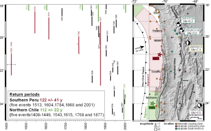
The last heavy earthquake seaward of Iquique occurred in 1877 (reconstructed magnitude 8.8), caused a large tsumani and has a recurrence time of 122 +/- 22 years (see Comte and Pardo, 1991). The historical record over the last 500 years shows that earthquakes in the Iquique segment occur in close temporal association with the seismic activation of neighbouring seismotectonic segments (Fig. 3).
Fig. 3: Map of coastal Chile, Iquique segment, the Peru-Chile Trench, seismic record and active tectonic structures. Unpublished, Source: GFZ Potsdam
In the southerly and northerly neighbourhood large earthquakes occurred in the past decades (Antofagasta 1995, South Peru 2001, Pisagua 2014). All this has led to an increase in seismicity in the Iquique segment. Since the rupture of the two directly adjoining segments (Antofagasta, Pisagua) the character of active deformation in the overriding plate in the Iquique segment has changed. Several previously inactive faults showed seismic activity since then, with magnitudes up to Mw 6.3 and ruptures up to the land surface. The seismogenic part of the plate boundary itself has increased activity, and a major earthquake (Tarapaca earthquake of 13.06.2005) was localized in the subducting plate at a focal depth of about 100 km.
All this indicates that an end of the present interseismic cycles is near or has been reached.
Cruise SO244/Leg 1 is dedicated to the marine geological exploration of those parts of the Iquique segment that have not been studied so far. Firstly, the geomorphological and geophysical base for long-term geodetic observation is to be laid. Secondly, the identification and mapping of active tectonic faults and submarine slumps and slides will give an overview of past movements of the seafloor. Thirdly, the high-resolution bathymetric mapping with the ship- based multibeam echosounder and with AUV ABYSS will provide a reference frame of the seafloor topography. After a future earthquake repeat surveys could then be used to quantify the mass movements during the event.
Almost the complete zone of seismic coupling between the Nazca and South American Plates is covered by the sea. To assess interseismic and permanent deformation, high-resolution mapping and observation of deformation and seismicity at the plate boundary, and the adjoining rock complexes is mandatory, and requires seagoing equipment. In contrast to the further progressed geological, geophysical and (satellite) geodetic exploration onshore, the trench and forearc in the Iquique segment is basically unstudied, requiring a timely, exploratory approach.
The proposed high-resolution bathymetric mapping in the Iquique seismotectonic segment between (Figure 2) for the first time documents the surface structure of the deep sea trench, and that of the lower and middle continental slope. Firstly, this is necessary to constrain the position and width of the outcrop of the zone of compression at the base of the continental slope, in comparison to the findings further south. This will reveal how contact deformation between the downgoing and overriding plates is localized and how it is partitioned. Together with seismic information, bathymetry holds crucial information for geomorphological and tectonic interpretation. Secondly those parts of the lower and middle continental slopes will be mapped, which are dominated by submarine mass wasting, be it caused by earthquakes or not. Based on
the data obtained, the volumes of the displaced materials may be quantified. Possibly, a relative chronology of larger mass wasting events can be established. This is important to estimate tsumanigenic potential by submarine sliding and slumping for the Iquique segment.
5 AGENDA OF THE CRUISE/PROGRAMM DER FORSCHUNGSFAHRT
The seafloor geodetic network to be deployed on Cruise SO244/Leg 2, immediately after the end of this cruise, will be positioned within an approximately 5 km wide strip from the shelf break to abyssal depths. A maximum water depth of 6 km cannot be surpassed for reasons of surveying with the AUV and system calibration. To determine the optimal location for the network we have applied a stepwise approach. First, we have mapped a larger part of the Chilean continental slope, the adjoining deep sea trench, and parts of the subducting oceanic Nazca Plate, using the ship-based EM122 multibeam system. The mapping area is broadly delimited by the 19°S and 22°S meridians, covering an area of approximately 18000 km2, see Figure 2). Mapping was generally conducted at a speed of 8 kn, with an aperture angle of the swath of 140°. Profile spacing was chosen to achieve optimal acoustic beam overlap wherever possible. We started mapping between the 20°30´S and the 21°30´S meridians, the target area for the AUV dives.
This was to make an early identification of the subareas for the installation of the seafloor geodetic network possible, which were then to be mapped at high resolution by AUV.
The criteria to choose the subareas for AUV mapping were the following (1) evidence for active faulting, deduced from the ship-based multibeam mapping; (2) fault scarps of moderate heights (max. 50 m) with terraces between the fault scarps not exceeding about 6° inclination. We aimed for a total of fifteen AUV dives within the expedition schedule at five locations, to allow a choice for the geodetic networks to be installed, and provide a minimum size for the installation of arrays comprising 6-8 stations. Using its 200 kHz multibeam sonar system, AUV ABYSS can map about 1 km2 per hour, flying 80 m above the seafloor at a speed of about 1.5 m/s. This secured sufficient overlap of the outer acoustic beams.
One dive had 16 or 14 hours duration, plus one hour for launch and recovery, and three hours for battery replacement. The two different durations of the dives related to the respective ages of the battery packs. We had two battery sets available, so that there was no loss of time for battery charging between deployments. Operating on a 24-hour turnaround, we were able to complete 15 dives within the expedition schedule. The break between two of the dives (Dives 7 and 8) was used to subject the autonomous wave glider to a short sea trial. This lasted about two hours and was finished successfully.
The retrieval of the 15 OBS deployed at the seafloor in the area of investigation at 9th and 10th December, 2014, was mostly conducted during transit from port (1 instrument), during initial mapping (6 instruments) and during time between AUV launch and recovery (3 instruments).
The northernmost five instruments made a dedicated necessary as far north as 19°S. Transits between these and all other OBS locations were in mapping mode (8 kn) to optimize use of the ship time and operative schedule for mapping. All fifteen instruments were successfully recovered from the seafloor
6 SETTING OF THE WORKING AREA/BESCHREIBUNG DES ARBEITSGEBIETES The Northern Chile – Southern Peru trench and forearc system has some features that make it unique among the subduction zones found on modern Earth. Since the recognition of the fact that old (i.e. Jurassic and Cretaceous) rocks crop out directly at the Pacific shore of south America (e.g. Rutland, 1971; Miller, 1970), this subduction zone has served as a showcase example of the process of tectonic erosion (e.g. von Huene et al., 1999). Tectonic erosion removes material from the front and base of the overriding plate, leading – at the same time – to subsidence and to the steepening of the slope angle of the marine forearc.
Tectonic erosion comes about when a topographically rough plate is subducted (see e.g.
Behrmann et al., 1994). This is the case when the downgoing plate has (1) a pronounced horst- and-graben fabric that is related to ocean floor spreading processes, (2) a lack of cover by marine pelagic and hemipelagic sediments, and (3) little or no sediment supply from the overriding plate into the deep sea trench. All three phenomena are documented for the Northern Chile/Southern Peru Trench (von Huene & Ranero, 2003), and were interpreted to constrain a regime of high friction along the east-dipping plate boundary fault. High basal friction, in turn, constrains a high angle of taper (Davis et al., 1983) and, thus, a steep slope of the continental forearc of the overriding plate. The shape changes induced by tectonic erosion lead to oversteepening, and the response is subhorizontal extension by a network of seaward and landward dipping normal faults (e.g. Geersen et al., 2015). Further south, seaward of the Mejillones Peninsula, normal faulting is indeed a characteristic of the upper and middle continental slope (von Huene & Ranero, 2003). Further seaward there is a mid-slope terrace that is transected by less or no normal faults, and the lower slope immediately above the subducting Nazca Plate is dominated by pervasive deformation of what could be crushed basement rocks.
Another characteristic of the Northern Chile forearc ist he presence of high-angle reverse faults (Gonzales et al., 2015), spatially connected with the so-called Arica Bend (e.g. Allmendinger et
al., 2005), which is the concave-seaward portion of the subduction zone. These reverse faults strike at high angles to the plate boundary and the coastline, and indicate that the overriding South American plate is in a state of along-arc compression (Gonzales et al., 2015).
Concave-seaward overthrusting at a subduction zone is a rare case on Earth, but the Andean example, termed the Bolivian Orocline ( following Isacks, 1988) seems to have persisted for a long time and continues to impose a pattern of clockwise and counterclockwise tectonic rotations around vertical axes on-land (e.g. Allemendinger et al., 2005). Oroclinal bending imposes the pattern of more or less trench-normal reverse faults in the Coastal Cordillera and it is an open question whether this pattern of faults extends seaward from the coast into the forearc. Based on seismological evidence the latter authors speculated that a trench-normal reverse fault may have played a role in the mechanical unclamping of the plate boundary thrust in the 1 April 2014 Pisagua earthquake (Schurr et al., 2014; Yagi et al., 2014; Kato and Nakagawa, 2014).
7 WORK DETAILS AND FIRST RESULTS/BESCHREIBUNG DER ARBEITEN IM DETAIL EINSCHLIESSLICH ERSTER ERGEBNISSE
7.1 Ship-based mapping with EM122 Multibeam Echosounder 7.1.1 Method
TFS SONNE is equipped with a Kongsberg Maritime EM122 multibeam echosounder operating at 12 kHz and covering water depths from 20 metres up to full ocean depth. Two different transmission pulses can be selected: a CW (Continuous Wave) or FM (Frequency Modulated) chirp. The sounding mode can be either equidistant or equiangle, depending on operation preferences and requirements. The EM122 system can be operated in single-ping or dual-ping mode, where one beam is slightly tilted forward and the second ping slightly tilted towards the aft of the vessel. The whole beam can also be inclined towards the front or the back, and the pitch of the vessel can be compensated dynamically. The EM122 system produces 432 beams covering an opening angle of up to 150°. The opening angle, however, can be reduced, if required.
The transducers of the EM122 system of RV Sonne are mounted in a so-called Mills cross array, where the transmit array is mounted along the length of the ship and the receive array is mounted across the ship length. The transmit array is about 16m long and can produce a beam with a maximum width of 150° across the ship and 0.5° along the ship. The receive array is
about 8m long and can produce a beam with a width of 30° along the ship and 1° across the ship. As a result the beams for producing the soundings have a size of 0.5° along and 1° across the ship. TFS SONNE is the first vessel with such a transducer array. Other systems are of a 1°
x 1° design. Considering that the outermost beams are noisy when using the maximum transmit width of 150°, this was reduced to a fixed value of 140° for the whole cruise. This means that in general the swath covered was a function of depth only: w=2´d´tan(140°/2) or roughly 5.5´d, where w is the swath width and d is the water depth. The number of soundings acquired in every ping cycle is 432. This implies that the spacing between soundings for one swath is equal to 5.5d / (432-1) = 0.01275d. As an example at 1,000m water depth spacing between adjacent soundings is 12,7m and at 6,000m water depth spacing is 76.5m. This is the resolution across the track. On the other hand, the ping rate depends on the water depth and is greater or equal to TWT=2´d/C, where C is the sound speed in the water column. The distance between one ping and the next one depends on the ping rate and on the ship’s speed (V), and is equal to TWT´V.
This is the resolution along the track.
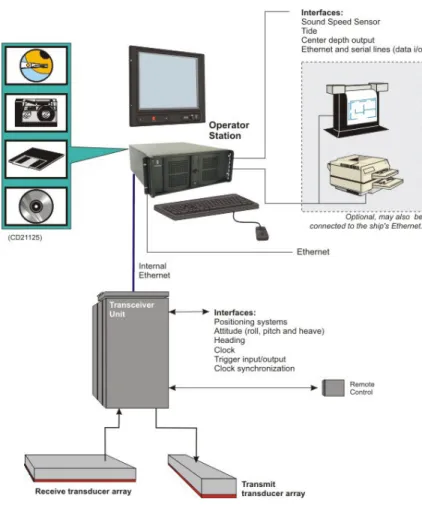
The echo signals detected from the seafloor go through a transceiver unit (Kongsberg Seapath) into the data acquisition computer or operator station (Fig. 4). In turn, the software that handles the whole data acquisition procedure is called Seafloor Information System (SIS). In order to correctly determine the point on the seafloor, where the acoustic echo is coming from, information abouth the ship's position, movement and heading, as well as the sound velocity profile in the water column are required.
Positioning is implemented onboard TFS SONNE with conventional GPS/GLONASS plus differential GPS (DGPS) by using either DGPS satellites or DGPS land stations, resulting in quasi-permanent DGPS positioning of the vessel. These signals also go through the transceiver unit (Seapath) to the operator station. However, during the SO244 Leg 1 cruise we were located outside DGPS satellite coverage and most of the DGPS land stations were too far away from the ship (2,000km or more).
Ship's motion and heading are compensated within the Seapath and SIS by using a Kongsberg MRU 5+ motion sensor. Beamforming also requires sound speed data at the transducer head, which is available from a Valeport MODUS SVS sound velocity probe. This signal goes directly into the SIS operator station. Finally, a sound velocity profile for the entire water column can be obtained from either a sound velocity probe or from a CTD (conductivity, temperature and density) probe. The temperature (T), salinity (S) and pressure (p) data acquired by any CTD (conventional or mounted on the AUV) can be converted into sound speed by using a sound
speed function C(S,T,p), such as TEOS-10 (Thermodynamic Equation of Seawater 2010, www.teos-1O.org).
Fig. 4: Configuration drawing of the EM122 system units and interfaces.
In addition to bathymteric information the EM122 system registers the amplitude of each beam reflection as well as a sidescan signal for each beam (so-called snippets). The EM122 system also allows recording the entire water column. The amplitude signals corresponds to the intensity of the echo received at each beam. It is registered as the logarithm of the ratio between the intensity of the received signal and the intensity of the output signal, which results in negative decibel values. For each ping EM122 records 432 backscatter signal values. The water column data correspond to the intensity of the echoes recorded from the instant the output signal is produced. All echoes coming from the water column, the seabed and even below the seabed are recorded for each beam. When the water column data of one ping is divided into a starboard and a port subsets, one can produce two traces, one for each subset. Each trace is built up as a time series in which for each time the highest amplitude is selected from all beams. Then the
starboard and the port traces are joint together. In the case of EM122 the side scan sonar data acquired in each ping consists of 1024 pixels.
7.1.2. Data
7.1.2.1. Bathymetry
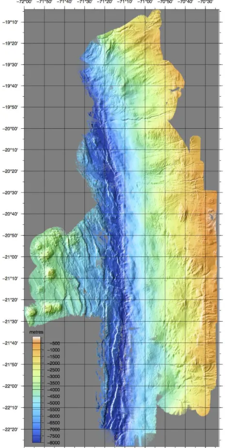
During cruise SO244 leg 1 the following settings of the Simrad EM122 system were used. The pulse was FM, ping mode was set to equidistant, dual ping mode was set to dynamic, and depth mode was set to automatic. The beam angle was reduced to 140° during most of the survey, except for a dedicated survey on the outer rise and another survey on the mid-slope, where the beam angle was reduced even further to 120° in order to increase resolution. The beam was initially tilted forward by 5° in order to avoid specular interferences of side lobes in the nadir region. This tilt angle was later reduced to 2°, as no problems with the near nadir pings were observed. Survey speed was generally 8 knots (sometimes 9 knots). Data were acquired continuously, except for OBS recovery and AUV deployment and recovery stations. During transit recording continued despite higher ship's speed. Water column data were recorded throughout the survey. Two CTD casts (Fig. 5) were used for water sound velocity profiles: one at the beginning of the survey on October 31 at 15:12 UTC in the southwestern corner of the study area at 21°99.978S and 71°14.996N, and a second CTD on November 12 at 23:43 UTC in the northern part of the survey area at 19°49.694S and 71°0.091N. Additional sound velocity profiles are available for post-processing corrections from the AUV dives. A total of 35000 km² of the continental margin offshore northern Chile was mapped in detail (Fig. 6) during the cruise.
This roughly corresponds to the size of Land Baden-Württemberg, one of the German Federal States.
The Simrad EM122 system was running stable throughout the cruise, except for rare interferences (twice) with the Parasound system in shallow water. These interferences resulted in the loss of the outer beams (Fig. 7) and required a restart of both the hardware and the software. Additional problems were encountered in deep water with a temporary but prolonged loss of the bottom detect resulting in a loss of useful soundings and consequently a gap in the data acquisition (Fig. 8). A clear reason for this behaviour is not known, but the combination of the overall tilt of beams, the local slope and scattering behaviour of the seafloor might result in strong specular reflection of the signal away from the transducer. This was the main reason for reducing the tilt angle. Finally, the system produces very good data except for the outer sector
that shows strong „wobbling“ of the beam from one ping to another (Fig. 9). This effect is particularly strong in deep water, but remained visible throughout the survey.
Fig.5: Sound velocity profiles of the water column, computed from CTD1 and CTD2 data.
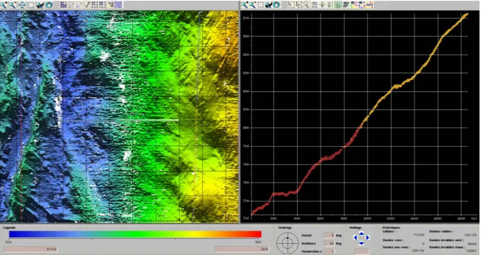
Data processing has been carried out onboard using different software packages (CARIS HIPS and SIPS, MB Systems and mainly Caraibes). Within Caraibes a triangulation filter with 3 iterations was applied in order to eliminate outliers, and the sounding data were then cleaned manually for further elimination of erroneous soundings. The data were subsequently gridded with Caraibes using a near-neighbour algorithm that takes into account four neighbouring cells, eliminates cells with less than two soundings per cell, and interpolates for 2 rows/columns. The soundings were also exported as xyz-data and gridded with GMT using a similar algorithm but no interpolation. The entire survey area was gridded with a 75 metres grid cell size and shows a big improvement over previous data (Fig. 10). The data from cruise SO244 leg 1 provide more detail and features appear much sharper.
Fig. 6: Shaded relief map of the continental slope offshore northern Chile showing the extent of area mapped during SO244 Leg1.
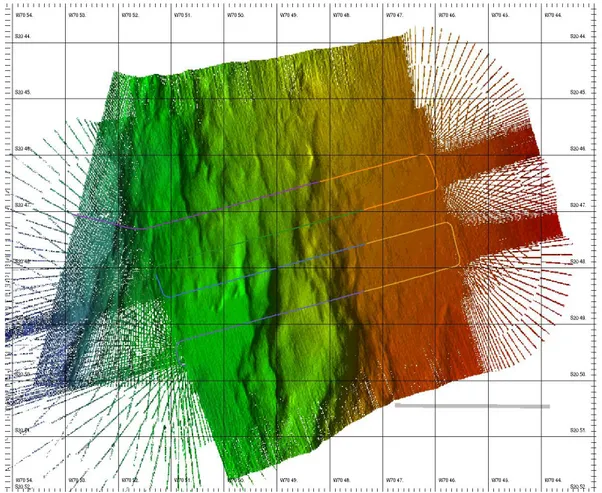
For AUV area 1, where a dedicated Parasound survey with closely spaced lines and 4 knots survey speed provided a high soundings density, a grid with 25 metres grid cell size could be calculated in roughly 2500 metres water depth (Fig. 11). Similar or even smaller grid cell sizes are possible in water depth shallower than 1000 metres, but would require additional editing of the data.
Fig.7: Screenshot of Caraibes editing tool showing the loss of outer beam registration.
Fig. 8: Screenshot of Caraibes editing tool showing the loss of correct bottom detection. Yellow dots show soundings that are rejected by the Simrad acquisition software.
Fig. 9: Screenshot of Caraibes editing tool showing the „wobbling“ of outer beams.
Fig. 10: Comparison of bathymetric data obtained during cruise SO244 Leg 1 and previous multibeam bathymetry data.
Fig. 11: Screenshot of Caraibes editing tool showing a 25m grid in 2500 metres water depth.
A preliminary morpho-structural analysis of the data has been carried out on board in order to choose suitable targets for the deployment of one or several Geodesy arrays. The focus for this analysis lay on active tectonic structures (faults in partcular). A whole set of slope parallel faults is present along the mid-slope region (Figs. 12, 13 and 14), where the first AUV deployments took place. If the whole margin is considered, only few areas show the presence of small intra- slope basins, where the seafloor is much smoother than in surrounding areas (Fig. 12). The trench also does not show widespread sediment accumulations, but only isolated, sediment- filled basins (Fig. 15). The oceanic plate, on the other hand, clearly displays a fabric generated at the spreading axis and running at an angle to the trench, as well as a few faults running parallel to the trench (Fig. 15). Some seamounts with well-developed craters are also present on the outer rise. Further to the south, large horst-and-graben structures run parallel to the trench axis (Fig. 16). The upper slope is dissected at irregular interval by small canyons (Figs. 12 and 13).
Fig.12: Shaded relief map of the eastern central part of the study area.
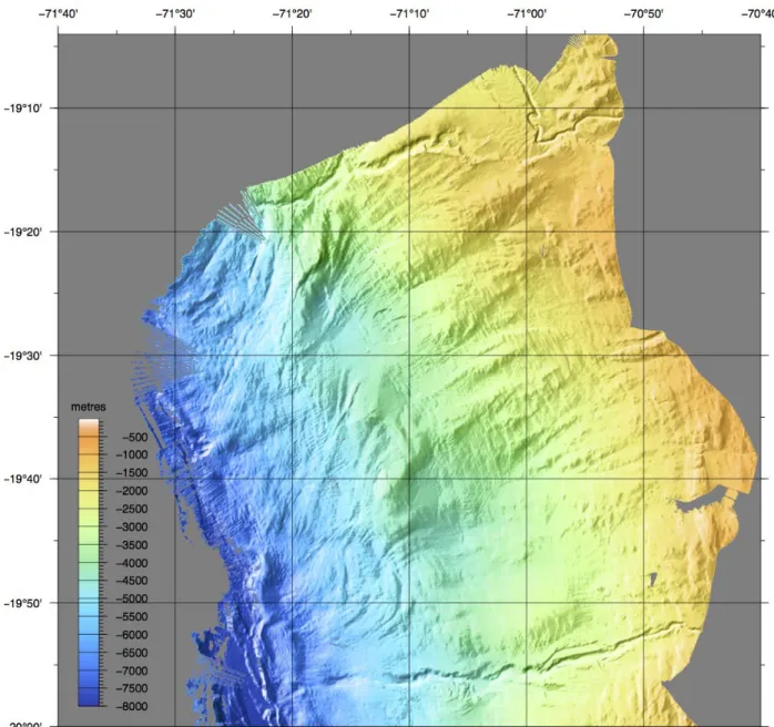
Fig. 13: Shaded relief map of the northern part of the study area.
Fig. 14 (previous page): Shaded relief map of the south-eastern part of the study area.
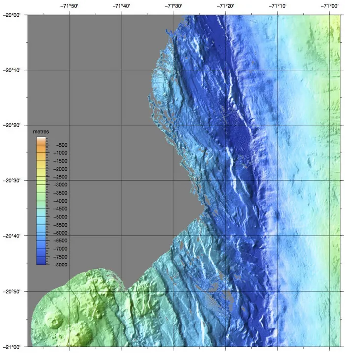
Fig. 15: Shaded relief map of the western central part of the study area showing features on the lower slope, the trench and the outer rise.
Fig. 16 (next page): Shaded relief map of the south-western part of the study area.
7.1.2.2 Backscatter
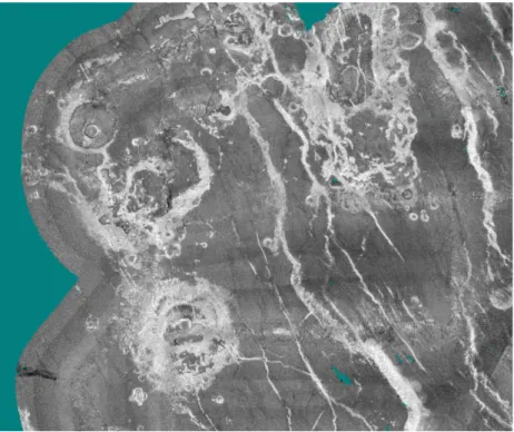
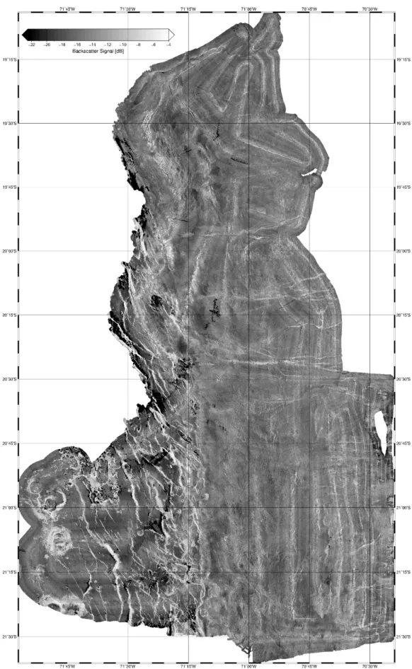
The backscatter (amplitude) signal is stored and preprocessed automatically by the Kongsberg software Seafloor Information System (SIS), including altitude processing, time varying gain (TVG) and angle varying gain (AVG). Backscatter data were processed onboard using CARIS Hips&Sips version 9.0.14. A grid with a resolution of 30m grid cell size was computed, but this produces many gaps in deep water (Fig. 17), because CARIS does not interpolate in a strict sense but averages spatially at the grid nodes. In order to fill the gaps, the backscatter signal data from very deep waters were exported to Global Mapper version 15.2.3 to be gridded including interpolation (Fig. 18). Finally, the gridded data from CARIS and Global Mapper was merged together in ASCII files for producing GMT grids. At the very end, a histogram of the data was produced in order to construct a gray scale for plotting the backscatter data. The histogram shows the data in class intervals, such as percentiles. After trial and error it was decided to produce a gray scale based on the data that range between the 1% and 99% percentiles (Fig.
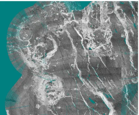
19). These data well underline the network of fault scarps on the oceanic plate that have high backscatter intensity, as well as submarine canyons dissecting the entire slope in the northern part of the study area (Fig. 19).
Fig. 17: Backscatter data gridded with CARIS, just spatial averaging. High backscatter is white.
Fig. 18: Backscatter data gridded with CARIS and Global Mapper merged together. Interpolation successfully fills many gaps without introducing artefacts. High backscatter is white.
Fig. 19: Map of backscatter data for the northern and central study areas. High backscatter is white.
7.1.2.3 Water column
The EM122 multibeam echosounder produces a second type of raw data files with extension
*.wcd, which stores water column data. These files were imported into Fledermaus version 7.2 module FMMidwater to produce Generic Water Column (.gwc) files. Fledermaus has 3 different display options for water column data: fan (show all beams of one ping, Fig. 20); beam (show one single beam for an entire profile; and stacked (show a stack of all beams inside a ping, Fig.
21). The EM122 produces 288 beams and for the present analysis the beam option was used and applied to the beam number 144, which corresponds to the nadir direction (Fig. 22). This is the most reliable beam, because along this direction the echoes are the strongest. This beam was exported with the format .sd to be displayed with Fledermaus on top of the bathymetry. This procedure can be done in chunks of data to avoid memory problems. The last step is the longest one, which is to visually analyze the .sd files one after another for detecting anomalies in the water column, such as plumes emerging from the seafloor. The task could not be carried out in detail onboard, but recurrent images of the deep plancton layer were observed (see Fig. 21).
Fig. 20: Display of water column data with Fledermaus using the fan option (across the track).
The beams are recorded radially from the origin, at the apex of the diagram.
Fig. 21: Display of water column data with Fledermaus using the stacked option (along the track).
Fig. 22: Display of water column data on top of bathymetry with Fledermaus using the beam option applied to beam 144 (nadir direction along the track).
7.2 Sub-bottom profiling using Parasound
7.2.1 Method
The hull-mounted parametric sub-bottom profiler PARASOUND DS3 (Atlas Hydrographic) was operated on a 24-hour schedule to provide high-resolution information on the uppermost 50-100 m of the sub-seafloor. The general description made here is based on the SO241 Cruise Report (Berndt et al., 2015). PARASOUND DS3 works as a narrow beam sediment echo sounder, providing primary high frequencies of 18 (PHF) and adjustable 18.5 – 28 kHz, thus generating parametric secondary frequencies in the range of 0.5 – 10 kHz (SLF) and 36.5 – 46 kHz (SHF) respectively. The secondary frequencies develop through nonlinear acoustic interaction of the primary waves at high signal amplitudes. This interaction occurs in the emission cone of the high-frequency primary signals, which is limited to an aperture angle of 4° for the PARASOUND DS3. This narrow aperture angle is achieved by using an array of 128 transducers on a rectangular plate of approximately 1 m² surface area. The footprint size of the generated signal is 7% of the water depth and vertical and lateral resolution is significantly improved compared to conventional 3.5 kHz echo sounder systems.
The PARASOUND DS3 is an improvement of the former PARASOUND DS2 (Atlas Elektronik) and is installed on TFS SONNE since 2014. The system provides features like recording of the 18 kHz primary signal and both secondary frequencies, continuous recording of the whole water column, beam steering, different types of source signals, and signal shaping. Digitization is carried out at 96 kHz to provide sufficient sampling rates for the high secondary frequency. A down-mixing algorithm in the frequency domain is used to reduce the amount of data and allows for data distribution via Ethernet.
During the entire cruise a SLF of 4 kHz was recorded in order to provide a good balance between signal penetration and vertical resolution. The PHF 18 kHz signal was also recorded permanently, but the high frequency data were not further processed and investigated during the cruise. All raw data were stored in the ASD data format (Atlas Hydrographic), which contains the data of the full water column of each ping as well as the full set of system parameters.
Additionally a 500 m-long reception window centered on the seafloor was recorded in the compressed PS3 data format after mixing the signal back to a final sampling rate of 24 kHz. This format is widely used and the limited reception window provides a detailed view on the subbottom structures. As the two-way travel time in deeper water is long compared to the length of the reception window, the Parasound System sends out a burst of pulses at 400 ms intervals,
until the first echo returns. The coverage of this discontinuous mode depends on the water depth and produces non-equidistant shot distances between bursts.
All data were converted to SEG-Y format during the cruise using the software package ps32sgy (Hanno Keil, Universität Bremen). The software allows generation of one SEG-Y file for longer time periods. We usually created SEG-Y files for 1-h long periods. The SEG-Y data was then loaded to the seismic interpretation software HIS Kingdom. This approach allowed us to depict sea floor morphology variations, sediment coverage, and sedimentation patterns along the ship’s track. The system worked reliably most of the time during the cruise, but had to be rebooted every 2-3 days after major program crashes, resulting in data gaps between 10 minutes and a couple of hours.
7.2.2 Data
Parasound data collection was carried out at variable ship speeds ranging from 4 to 12 nm/h.
Signal quality was good for 4 to 8 nm/h, but even at 12 nm/h decent parasound profiles could be obtained. Sub-seafloor penetration was much more controlled by two other parameters, seafloor morphology and sediment thickness. Large parts of the studied area are characterized by slope gradients in excess of 5° with peak values reaching 20-30°.
Fig. 21: Data example: N-S trending Parasound profile along the upper continental slope
The steep slopes in combination with the widespread absence of a sedimentary slope cover significantly reduce the sub-seafloor penetration of the Parasound signals across most of the study area. A good resolution of the upper 20-50 m of the sub-seafloor was only achieved in some areas of the middle and upper continental slope, where local sedimentary basins or drift sediment deposits are located (see Fig. 21 for a data example). During most of the cruise the ship track was oriented parallel to the slope (~i.e. N-S direction) in order to increase the spatial coverage of the area mapped with the multibeam system (see Fig. 2 for ship track). As a direct consequence, the majority of the tectonic structures in the study area, which strike in N-S direction (compare chapter multibeam) are not cut and thereby imaged in the Parasound data.
Complementary to the multibeam bathymetry, parasound profiling displays that areas with a rugged surface morphology go along with very thin (meter-scale) or inexistent cover sediments.
In contrast, smooth areas with horizontal or only slightly inclined seafloor surface mostly correspond to considerable sediment thicknesses, in places more than several tens of meters.
Local smooth surface areas with higher sediment thicknesses are mostly found on the middle and upper continental slope, but are frequently interrupted by rugged surface areas with little or no sediment cover.
Fig. 22: Data example: E-W trending Parasound profile across AUV diving area 1. East is to the left.
The rugged surface areas also dominate the lower continental slope and the trench. In the entire study area fault scarps are well visible and ubiquitous in the bathymetric data. However, mostly the underlying faults are not resolved in the Parasound data due to little sediment coverage and steep slopes, or a combination of both effects.
For a detailed view into the sub-surface of AUV Mapping Area 1 (see below) we collected five Parasound profiles (see Fig. 22 for an example) perpendicular to the slope in Area 1 (mid-slope;
see Fig. 2) in order to obtain information on the nature of the fault that underlies the seafloor scarp. Directly landward of the escarpment shallow sediment layers are repeatedly offset by a series of seaward dipping faults (left in Fig. 22). In contrast, the shallow sediments seaward of the fault escarpment are horizontally layered and not offset by major faults (right in Fig. 22).
7.3 AUV ABYSS Mapping 7.3.1 Method
The Autonomous Underwater Vehicle (AUV) ABYSS (built by HYDROID Inc.) from GEOMAR can operate in water depths up to 6000 m. The system comprises the AUV itself, a control and workshop container, and a mobile Launch and Recovery System (LARS) with a deployment frame that was installed at the starboard side on the afterdeck of R/V Sonne. The self-contained LARS was developed by WHOI to support ship-based operations so that no Zodiac or crane is required for launch and recovery. The LARS is mounted on steel plates, which are screwed to the deck of the ship. The LARS is configured in a way that the AUV can be deployed over the stern or port/starboard side of the German medium and ocean-going research vessels. The AUV ABYSS can be launched and recovered at weather conditions with a swell up to 2.5 m and wind speeds of up to 6 Beaufort. For the recovery the nose float pops off when triggered through an acoustic command. The float and the ca. 19 m recovery line drift away from the vehicle so that a grapnel hook can snag the line. The line is then connected to the LARS winch, and the vehicle is pulled up. Finally, the AUV is brought up on deck and secured in the LARS. The AUV missions were planned based on the shipboard bathymetry, acquired immediately befor the diving missions.
During cruise SO244-1 fifteen missions were flown by ABYSS (See Appendix 11.B).
Fig. 23: Launch and Recovery System in use while recovering AUV (Photo: Inken Preuss)
Fig. 24: AUV system composition on board Sonne during SO244-1 (Photo: Inken Preuss)
Fig. 25: AUV Abyss ready for launch in the LARS (Photo: Henry Robert)
7.3.2 Data processing
AUV multibeam data were acquired during 15 dives focussed on 5 larger areas (see Fig. 2) picked from the ship EM122 multibeam data. Raw data were acquired in .s7k format and converted to MBSystem .mb88 format. Multibeam and backscatter were acquired during all missions. Overall the data were of a high quality, with good navigation, few artifacts/areas of bad data and sufficient overlap (typically around 400m) to allow acurate merging. On three missions (207, 213 and 215) small sections of data were lost when the vehicle lost DVL. Raw bathymetric data were postprocessed using several software packages. Vehicle offsets (roll bias – 0.17, pitch bias – 1.32 and heading offset – 0.93) were applied using the mbset and mbprocess modules of MBSystem (Fig. 26). Additionally mbset was used to apply a navigational shift of 515m on a bearing of 280° to Abyss0211, and a shift of 455m on a bearing of 266° to Abyss0213, both of which had not recieved positional information at the beginning of the mission. These missions were then processed as normal. MBSystem was used to renavigate datasets to an internally consistent solution with the mbnavadjust module (Fig. 27). Then, datasets collected in the same area were merged together using the mbnavadjustmerge
function. During navigational processing .xyz data were periodically exported and the standard deviation of these points from the average surface checked to maintain data quality in QINSy Qloud and/or Fledermaus. Final combined grids were filtered and manually cleaned to remove bad data and spikes in QINSy before being positionally checked against the underlying EM122 bathymetry for consistency. As a result the entire combined grid for Abyss214-216 was shifted 390 m on a bearing of 233°. Final grids were produced with a pixel size of 2 m with MBSystem.
Fledermaus scene files and XYZ data of the final products were also provided.
Fig. 26: Screengrab from MBSystem navadjust module showing two sections of tied data.
Contour spacing is 2m and section length is 0.14 km.
Fig. 27: A section of Abyss0213 before (A) and after (B) processing with mbnavadjust.
7.3.3 Discussion of First Results
Abyss0204-0207 (Area 1; Fig. 28): The combined missions covered 34.9 km2 of normal faulted terrain on the continental slope focussed on the northern half of a long, westward dipping normal fault visible in the EM122 bathymetry. This fault, along with others stepping downwards to the west were imaged sucessfully by the surveys. Several terminate in an undisturbed sediment pond, suggesting ho recent movement, however, the largest shows a number of small (< 80 m across) mass wasting features. Erosional gullying is also visible atop this fault.
Abyss0208-0209 (Area 2; Fig. 29): The combined missions covered 16.9 km2 and targeted two eastward dipping scarps identified from the EM122 on the outer rise of the Nazca plate, approximately 100 km west of the first survey area. These scarps appear to be normal faults that cross cut the old volcanic terrain. Both were imaged sucessfully, however, there is little fine detail in the maps. The majority of the seafloor is very smooth suggesting it is sedimented and no obviously recently active features were observed.
Abyss0210-0213 (area 3; Fig. 30): Missions Abyss0210-0213 covered a total area of 32.2 34.9 km2 of continetal slope approximately 10 km east of the deepest part of the trench and 25 km west of Area 1 in water depths between 4970 m and 5858 m. The survey covers a ridge with approximately 500 m relief, trending 140°, that can be traced to the deepest part of the trench.
Fig. 28: Colour-coded ocean floor relief map of the Digital Elevation Model (DEM) derived from AUV dive multibeam data from Area 1. Lighting is from the SE.
The AUV data reveals a quite complex terrain consisting of several smooth, elongate highs with reliefs of between 10 and 30 m, which also trend 140° and numerous smaller structures with no clear alignment. Some appear to be faulted on their western side, and other smaller features may also be fault controlled, however, there is no clear evidence for recent tectonic deformation.
Fig. 29: Colour-coded ocean floor relief map of the DEM derived from AUV dive multibeam data from Area 2. Lighting is from the SE.
Abyss0213-0215 (Area 4; Fig. 31): Missions Abyss0213-0216 lie around 60 km south of Area 3 and 20 km east of the deepest part of the trench in water depths between 4210 m and 4835 m.
The data show the base of a rough, probably rocky slope in the north east corner, which corresponds to what appear to be several N-S trending, westward dipping fult scarps in the EM122 bathymetry. A second set of faults to the south are also imaged and appear smoother and more sedimented. The centre of the survey area is dominated by a sedimented plain with a few minor westward dipping faults. The western end is again characterised by larger structures, which in the South western corner appear to have two main orientations, 135- 315° and 16 - 196°, although only the N-S orientated ones show any large displacement. The terrain here is smoother than in the north eastern corner suggesting thicker sediment cover.
Abyss0217-0218 (Area 5): Missions Abyss0217 and 0218 cover 12.3 km2 in water depths between 1880 m and 2350 m. Area 5 is 60 km south of Area 1 and 25 km east of Area 4. The missions focus on an area where two scarps with different orientations (76 - 256° and 9 - 189°),
identified from the EM122 bathymetry, intersect. The N-S of these scarps is actually four normal faults that step down to the west and have some of the steepest dips (up to 40°) surveyed. The faulted terrain is faily rough, however the area at the base of the scarps is characterised by a smooth, flat plain, which is most likely a sediment pond. At the time of reporting data from these missions had not finally been processed, and are, thus, not included here.
Fig. 30: Colour-coded ocean floor relief map of the DEM derived from AUV dive multibeam data from Area 3. Lighting is from the SE.
Fig. 31: Colour-coded ocean floor relief map of the DEM derived from AUV dive multibeam data from Area 4. Lighting is from the SE.
7.4 Retrieval of Ocean Bottom Seismometers
During the period of 09.12. - 10.12.2014, fifteen GEOMAR Ocean Bottom Seismometers (OBS) were deployed in collaboration with the Chilean NAVY, by their vessel OPV TORO at the locations given in Fig. 32, and in Table 1.
The buoyancy body is made of syntactic foam and is rated, as are all other components of the system (Fig. 33), for a water depth of up to 6000 m. The release unit is a K/MT562 made by KUM GmbH. Communication with the instrument is possible through acoustic signal from the releaser deck units AMD200R and 8011M made by KUM, which trigger the release transponder to drop the weight of 60 kg. As weight pieces of railway tracks (untreated steel) were used. The sensors are OAS and HTI hydrophones and Owen seismometers connected to the pressure
tube and the recording unit, an MLS recorder of SEND GmbH. As energy source Li-batteries were used.
Fig. 32: Locations of GEOMAR OBS long-term deployment offshore Northern Chile. Blue squares represent OBS positions; red stars show the locations of the 01.04.2014 Mw 8.2 Pisagua earthquake and the largest aftershock (Mw 7.7).
The principal setup of the OBS (see Figure 2) consists of a hydrophone, a geophone/
seismometer, a pressure tube containing the recording unit and the energy source, a weight fixed to a releaser unit, and a flash light, radio beacon, flag for better sighting and a swimming line, all of them mounted on a steel frame, which holds the buoyancy body.
Fig. 33: GEOMAR OBS during retrieval
All 15 OBS were retrieved successfully during the SO244-1 cruise and had recorded a total 117,1 GB of data over a time period of approximately 11 months. For more details see Table 1.
SO244 station #
TORO Station #
Latitude (deg)
Longitude (deg)
Deployment Date
Retrievel Date
Depth (m) File size (GB) 244/1_45
OBS 01 19° 05.95' 70° 54.15' 09.12.14 12.11.15 1498 8.2 244/1_42
OBS 02 19° 20.99' 71° 21.02' 09.12.14 11.11.15 2411 9.2 244/1_47
OBS 03 19° 29.99' 70° 59.99' 09.12.14 13.11.15 2352 7.6 244/1_41
OBS 04 19° 45.01' 71° 09.97' 09.12.14 11.11.15 4437 9,5 244/1_49
OBS 05 19° 44.99' 70° 45.16' 09.12.14 12.11.15 1171 7.4 244/1_23
OBS 06 20° 00.57' 70° 52.83' 09.12.14 06.11.15 2124 8.0 244/1_28
OBS 07 20° 15.01' 71° 01.75' 09.12.14 07.11.15 3910 7.0 244/1_21
OBS 08 20° 14.96' 70° 42.04' 09.12.14 06.11.15 1490 9.5 244/1_4
OBS 09 20° 29.96' 70° 50.99' 09.12.14 01.11.15 2509 7.3 244/1_8
OBS 10 20° 45.11' 70° 59.73' 09.12.14 02.11.15 3892 7.1 244/1_12
OBS 11 20° 44.92' 70° 42.07' 09.12.14 03.11.15 2139 5.4 244/1_10
OBS 12 20° 59.95' 70° 48.99' 09.12.14 02.11.15 3002 9.5 244/1_6
OBS 13 21° 21.01' 70° 58.19' 10.12.14 01.11.15 4525 7.1 244/1_14 OBS 14 21° 44.99' 70° 48.16' 10.12.14 31.10.15 3890 7.0 244/1_1 OBS 15 21° 20.09' 70° 39.01' 10.12.14 03.11.15 2059 7.3
Table 1: deployment and retrieval information for the long–term OBS deployment offshore Northern Chile.
7.5 Wave Glider Test Run
The Wave Glider is an autonomous, environmentally powered ocean-going platform by Liquid Robotics. The Wave Glider is composed of two parts (see Fig. 34): the float contains all sensors and communication units, and the sub hangs 6 meters below the float. The separation is due to the float, and makes the latter experience more wave motion than the sub. This difference allows wave energy to be harvested to produce forward thrust.
The Wave Glider is equipped with satellite communication systems for remote transmittal of data, plus global positioning system, weather station and a hydrophone to communicate with the
acoustic geodetic seafloor stations to be monitored. The necessary power is provided by solar panels, which recharge the Li-batteries located in the float.
The Wave Glider can be programmed for autonomous operation, or can be controlled by a pilot over the Internet.
During the SO244/1 Cruise the GEOMAR Wave Glider was tested in the Pacific Ocean for the first time. The test was limited to the functionality of communication and navigation. The Wave Glider was set in water at 17:35 UTC and recovered at 19:15 ( see Table C1 in Appendix C).
During this time the Wave Glider navigated around the Vessel the successfully (Fig. 35).
Fig. 34: The GEOMAR Wave Glider in operation during the test run
Fig. 35: Positions of the Wave Glider during the test run
8 ACKNOWLEDGEMENTS/DANKSAGUNG
We thank the Master and Crew of TFS SONNE for their unrivalled support of the scientific work at sea, for their high motivation and highly professional work, which laid the foundation for a perfect expedition. The Leitstelle Deutsche Forschungsschiffe in Hamburg, the German Ministery for Education and Research (BMBF), and Briese Schiffahrts GmbH & Co. KG are all acknowledged for the support and practical assistance that have made Cruise SO244 Leg 1 possible. We thank SHOA, Valparaiso, Chile, and the German Ministery of Foreign Affairs for seamless communication in connection with obtaining the necessary research permits.
9 REFERENCES/LITERATURVERZEICHNIS
Allmendinger RW, Samlley Jr. R, Bevis M, Caprio H, Brooks B (2005) Bending the Bolivian Orocline in real time. Geology, 33, 905-908, doi: 10.1130/G21779.1
Behrmann JH, Lewis SD, Cande S, ODP Leg 141 Scientific Party (1994) Tectonics and geology of spreading ridge subduction at the Chile Triple Junction; a synthesis of results from Leg
141 of the Ocean Drilling Program. Geol. Rundschau, 83, 832-852.
Berndt C (2015) RV SONNE 241 Cruise Report / Fahrtbericht, Manzanillo, 23.6.2015 – Guayaquil, 24.7.2015 : SO241 - MAKS: Magmatism induced carbon escape from marine sediments as a climate driver – Guaymas Basin, Gulf of California GEOMAR Helmholtz Centre for Ocean Research Kiel, 74 pp. DOI 10.3289/CR_S241.
Comte D, Pardo M (1991) Reappraisal of great historical earthquakes in the northern Chile and southern Peru seismic gaps. Natural Hazards, 4, 23-44.
Davis D, Suppe J, Dahlen FA (1983) Mechanics of fold-and-thrust belts and accretionary wedges. Journal of Geophysical Research, 88, 1153-1172.
Geersen J, Ranero CR, Barckhausen U, Reichert C (2015) Subducting seamounts control interplate coupling and seismic rupture in the 2014 Iquique earthquake area Nature Communications, 6 . p. 8267. DOI 10.1038/ncomms9267.
Gonzales G, Salazar P, Loveless JP, Allmendinger RW, Aron F, Shrivastava M (2015) Upper plate reverse fault reactivation and the unclamping of the megathrust during the 2014 northern Chile earthquake sequence. Geology, 43, p. 671-674, doi: 10.1130/G36703.1 Isacks, B.L., 1988, Uplift of the central Andean plateau and bending of the Bolivian orocline.
Journal of Geophysical Research, 93, 3211–3231.
Kato A, Nakagawa S (2014) Multiple slowslip events during a foreshock sequence of the 2014, Chile Mw 8.1 earthquake. Geophysical Research Letters, 41, 5420–5427, doi:10.1002 /2014GL061138.
Miller H (1970) Das Problem des hypothetischen Pazifischen Kontinentes gesehen von der chilenischen Pazifikküste. Geol. Rdsch., 59, 927-938.
Rutland RWR (1971) Andean orogeny and ocean floor spreading. Nature, 233, 252-255.
Schurr B, et al. (2014) Gradual unlocking of plate boundary controlled initiation of the 2014 Iquique earthquake. Nature, 512, 299–302,
doi:10.1038/nature13681.
von Huene R, Weinrebe W, Heeren F (1999) Subduction erosion along the North Chile margin.
J. Geodyn., 27, 345-358.
Von Huene R, Ranero CR (2003) Subduction erosion and basal friction along the sediment- starved convergent margin off Antofagasta, Chile. Journal of Geophysical Research, 108, 2079, doi:10.1029/2001JB001569
Yagi Y, Okuwaki R, Enescu B, Hirano S, Yamagami Y, Endo S, Komoro T (2014) Rupture process of the 2014 Iquique Chile earthquake in relation with the foreshock activity.
Geophysical Research Letters, 41, 4201–4206, doi:10.1002/2014GL060274.