catchment on Herschel Island (Yukon Territory, Canada)

(1)

ARTICLE

Summer rainfall dissolved organic carbon, solute, and sediment fluxes in a small Arctic coastal

catchment on Herschel Island (Yukon Territory, Canada)

Caroline Coch, Scott F. Lamoureux, Christian Knoblauch, Isabell Eischeid, Michael Fritz, Jaroslav Obu, and Hugues Lantuit

Abstract:Coastal ecosystems in the Arctic are affected by climate change. As summer rainfall frequency and intensity are projected to increase in the future, more organic matter, nutrients and sediment could be mobilized and transported into the coastal nearshore zones.

However, knowledge of current processes and future changes is limited. We investigated streamflow dynamics and the impacts of summer rainfall on lateral fluxes in a small coastal catchment on Herschel Island in the western Canadian Arctic. For the summer monitoring periods of 2014–2016, mean dissolved organic matter flux over 17 days amounted to 82.7± 30.7 kg km⁻² and mean total dissolved solids flux to 5252±1224 kg km⁻². Flux of suspended sediment was 7245 kg km⁻²in 2015, and 369 kg km⁻²in 2016. We found that 2.0% of suspended sediment was composed of particulate organic carbon. Data and hysteresis analysis suggest a limited supply of sediments; their interannual variability is most likely caused by short-lived localized disturbances. In contrast, our results imply that dissolved organic carbon is widely available throughout the catchment and exhibits positive linear relationship with runoff. We hypothesize that increased projected rainfall in the future will result in a similar increase of dissolved organic carbon fluxes.

Key words:permafrost, hydrology, lateral fluxes, hysteresis, climate change.

Résumé :Les écosystèmes côtiers dans l’Arctique sont touchés par le changement climatique. Comme la fréquence et l’intensité des pluies d’été sont censées augmenter à l’avenir, plus de matière organique, de substances nutritives et de sédiments pourraient être mobilisés et transportés dans les zones proches des côtes. Par contre, la connaissance quant aux processus actuels et quant aux changements futurs est limitée. Nous avons examiné la dynamique de débit d’eau et les impacts des pluies d’été sur les flux latéraux dans un petit

Received 3 May 2018. Accepted 5 July 2018.

C. Coch and H. Lantuit.Department of Periglacial Research, Helmholtz Centre for Polar and Marine Research, Alfred Wegener Institute, Telegrafenberg A45, Potsdam 14473, Germany; Institute of Earth and Environmental Science, University of Potsdam, Karl-Liebknecht-Straße 24/25, Potsdam 14476, Germany.

S.F. Lamoureux.Department of Geography and Planning, Queen’s University, Mackintosh-Corry Hall, Room E208, Kingston, ON K7L 3N6, Canada.

C. Knoblauch.Institute of Soil Science, Universität Hamburg, Allende-Platz 2, Hamburg 20146, Germany.

I. Eischeid.Norwegian Polar Institute, Framsenteret, Hjalmar Johansens gate 14, Tromsø 9296, Norway.

M. Fritz.Department of Periglacial Research, Helmholtz Centre for Polar and Marine Research, Alfred Wegener Institute, Telegrafenberg A45, Potsdam 14473, Germany.

J. Obu.Section of Physical Geography and Hydrology, Geologibygningen, University of Oslo, Sem Sælands vei 1, Oslo 0371, Norway.

Corresponding author:Caroline Coch (e-mail:caroline.coch@awi.de).

Mark L. Mallory currently serves as an Associate Editor; peer review and editorial decisions regarding this manuscript were handled by Greg Henry.

This article is open access. This work is licensed under a Creative Commons Attribution 4.0 International License (CC BY 4.0).

http://creativecommons.org/licenses/by/4.0/deed.en_GB.

Arctic Science Downloaded from www.nrcresearchpress.com by BIBLIO DES WISSENSCHAFTSPARKS on 11/22/18 For personal use only.

(2)

bassin hydrologique côtier de l’île Herschel dans l’ouest de l’Arctique canadien. Pour les périodes de surveillance d’été de 2014–2016, le flux moyen de matière organique dissoute au cours de 17 jours s’est chiffré à 82,7±30,7 kg km⁻²et le flux moyen du total de matière solide dissoute, à 5252±1224 kg km⁻². Le flux de sédiments en suspension était de 7245 kg km⁻²en 2015, et de 369 kg km⁻²en 2016. Nous avons constaté que 2,0 % de la composition de sédiments en suspension constituait du carbone organique en particules.

L’analyse des données et de l’hystérèse suggèrent un volume limité de sédiments; leur variabilité interannuelle est très probablement causée par des perturbations localisées de courte durée. Au contraire, nos résultats laissent penser que la matière organique dissoute est largement disponible partout dans le bassin hydrologique et montre une relation linéaire positive avec l’écoulement. Nous formulons l’hypothèse qu’à l’avenir les pluies accrues prévues entraîneront une augmentation semblable du flux de matière organique dissoute. [Traduit par la Rédaction]

Mots-clés :pergélisol, hydrologie, flux latéraux, hystérésis, changement climatique.

Introduction

Climate change has important impacts on terrestrial and marine Arctic ecosystems. As rainfall frequency and intensity are projected to increase in the future (Bintanja and Andry 2017), more organic matter, nutrients, and sediment could be mobilized and transported from coastal areas into nearshore zones of the Arctic Ocean. The eight largest Arctic Rivers cover 53% of the Arctic drainage basin, and contribute major fluxes of water and material to the Arctic Ocean (Holmes et al. 2002,2012;Peterson et al. 2002;Gordeev 2006;Wegner et al. 2015). The remaining 47% of the Arctic drainage basin is characterized by smaller watersheds, where very limited flux estimates are available.

Lateral transport of dissolved organic carbon (DOC), total dissolved solids (TDS), and suspended sediment (SS) is strongly influenced by permafrost coverage, ground ice, topogra- phy, soil and vegetation types, and varies across the Arctic region (Vonk et al. 2015;Tank et al. 2018). To investigate sources and flow pathways of a catchment, the dynamic relationship between discharge and hydrochemical concentration for separate hydrographs is stud- ied over time. Hysteresis refers to the cyclical pattern that forms when concentrations at a given discharge differ on the rising and falling limb of the hydrograph. Clockwise hysteresis loops are generally interpreted to indicate a limitation or a source close to the channel outflow. Anti-clockwise or counter-clockwise loops imply a source further away from the outlet, or a late availability of material (Klein 1984). Only few studies examine hysteresis patterns and fluxes of DOC, TDS, and sediment as summarized here.

DOC is positively correlated with discharge in subarctic locations. The hysteresis pattern there varies between studies showing a clockwise behaviour (Carey 2003;Spence et al. 2015) or an anti-clockwise relationship (Petrone et al. 2007). Rain events lead to a dilution of baseflow water and thus, to a decline of major ion concentrations (MacLean et al. 1999;Petrone et al. 2007). Hysteresis patterns for calcium and potassium are clockwise across catchments with varying permafrost coverage (Petrone et al. 2007). The majority of SS is transported during the snowmelt season (Braun et al. 2000;Forbes and Lamoureux 2005;Cockburn and Lamoureux 2008;Lamb and Toniolo 2016;Lamoureux and Lafrenière 2017), although high amounts of sediment may also be mobilized during summer rainfall events (Lewis et al. 2005;Dugan et al. 2012;Lamb and Toniolo 2016). Clockwise suspended sediment discharge hysteresis behaviour suggests a limitation and therefore rapid exhaustion of sediment that can be mobilized during rainfall (Dugan et al. 2009). As specific suspended sediment yield is known to increase with decreasing watershed size (Walling 1983;

Dedkov 2004;Fryirs 2013), small watersheds in the Arctic may cumulatively contribute more sediment to the Arctic Ocean than the large Arctic Rivers.

(3)

The knowledge about summer rainfall impacts on the release of DOC, TDS, and SS is limited and few studies report on these dynamics in continuous permafrost areas.

The objectives of this paper are therefore to investigate the dynamics of hydrology and hydrochemistry in a small coastal watershed on Herschel Island in the northwestern Canadian Arctic. More specifically, we aim at (1) determining characteristics of discharge associated with baseflow and summer rainfall and at (2) quantifying fluxes of DOC, TDS, and SS with regard to baseflow and rainfall events. The results will contribute to under- stand how similar watersheds in Low Arctic locations will respond to varying rainfall inputs that become increasingly important in the region (Bintanja and Andry 2017).

Study site

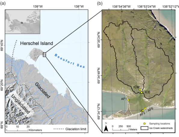
The Ice Creek West watershed (1.4 km²) is located on the eastern coast of Herschel Island at 69.58°N and 138.89°W (Fig. 1). It merges with an adjacent watershed to the east before draining into an alluvial fan and finally into the sea. Herschel Island covers an area of about 116 km²with a maximum elevation of 183 m above sea level and is situated in the Beaufort Sea off the Yukon Coast of Canada. The island is an ice-thrust moraine formed by the Laurentide Ice Sheet and it is characterized by the abundance of unconsolidated and fine-grained marine and glacigenic sediments (Mackay 1959;Pollard 1990;Fritz et al.

2012). The island is situated in the zone of continuous permafrost exhibits high ground

Fig. 1. Map showing (a) the location of Herschel Island and the glaciation limit along the Yukon Coast and (b) the Ice Creek watersheds with the locations for water sampling at the outflow of Ice Creek East (ICE) and Ice Creak West (ICW) and the alluvial fan (AF). Projection: UTM NAD 1983. Image base (b): GeoEye 2011 image.

(4)

ice contents amounting to 30%–60% of the entire island (Rampton 1982;Pollard 1990;Fritz et al. 2012). Ground temperature monitoring on the east side of the island reveals a mean annual ground temperature of−8 °C at zero amplitude depth of approximately 14.5 m (Burn and Zhang 2009).

The island’s coast is eroding rapidly and numerous retrogressive thaw slumps associated with the presence of ice-rich permafrost occur along the shore (Lantuit and Pollard 2008;

Radosavljevic et al. 2015). Mass wasting also occurs in the form of active layer detachments, thermal erosion gullies, or solifluction on the island and affects the soil organic carbon (SOC) storage (Obu et al. 2017).Smith et al. (1989)classify the soils on Herschel Island based on the Canadian system of soil classification. The island is dominated by organic cryosoils, whereas Turbic cryosoils (cryoturbation) and static cryosoils are present on beaches and spits where near-surface permafrost is absent. The vegetation on Herschel Island is classi- fied as lowland tundra (Smith et al. 1989;Myers-Smith et al. 2011), and can be assigned to subzone E (CAVM Team 2003) or the Low Arctic, respectively. Vegetation cover within the watershed is almost continuous and dominated byDryas-graminoid-forbcommunities.

In the upper flatter sections of the watershed, the landscape is characterized by Eriophorum vaginatumtussocks and soils rich in organic matter. Shrubs (Salixsp.) up to 1 m in height occur in terrain depressions and the creek confluence. Eroded slopes are quickly recolonized byPetasites frigidus,Artemisia tilesii, orSenecio congestus.

Environment and Climate Change Canada runs an automated weather station at Pauline Cove on Herschel Island (WMO ID: 715010) with temperature recordings since 1995. Records of precipitation are only available since 2004 and are often incomplete. The mean annual air temperature compiled from no-gap data months between 1995 and 2016 is−8.4 °C (Environment and Climate Change Canada 2018). Between 1926 and 1970, mean annual air temperatures have been stable in the Canadian western Arctic, followed by a total increase of 2.7 °C between 1970 and 2005. This increase of temperature is also reflected on Herschel Island where a deepening of the active layer by 15–25 cm has occurred between 1985 and 2005 (Burn and Zhang 2009).

The largest hydrological event of the year is snowmelt, which occurs in late May or early June, where the average monthly air temperatures are−3.4 and 4.2 °C, respectively. Freeze up of the active layer takes place by mid-November for most of the island (Burn 2012).

Methodology Weather data

During the field monitoring in 2015 and 2016, we installed a weather station in Ice Creek West collecting air temperature (BTF11/002 TSic 506;±0.1 °C accuracy), incoming solar radiation (UTK–EcoSens 11.6.6133.0051; error<10%), wind speed (Thies CLIMA 4.3519.00.173;

±0.5 m s⁻¹accuracy), and precipitation (tipping bucket gauge Young Model 52203; 0.1 mm per tip; accuracy±2%). Our station was located approximately 1 km away from the station run by Environment and Climate Change Canada.

There is a significant positive correlation (R²=0.85;p<0.05) between the two stations (Fig. A1). However, we find that the Environment Canada station underestimates the precipitation by 66% on average compared with our station in Ice Creek West. This may be related to the northwest (NW) wind pattern that is predominant during storms bringing more rain to our weather station in Ice Creek West. The linear regression formula (y=1.28+0.42) has been applied to the Environment Canada data to correct for this offset.

We also compared daily mean air temperature between both stations and find a near zero temperature gradient between both, which is why no corrections were applied to the Arctic Science Downloaded from www.nrcresearchpress.com by BIBLIO DES WISSENSCHAFTSPARKS on 11/22/18 For personal use only.

(5)

temperature data. Precipitation data are missing for the complete season of 2014 and also at the stations nearby Komakuk or Shingle Point.

Hydrology

Discharge was measured during summer months between 2014 and 2016. A cutthroat flume (w=0.2 m;l=0.7 m;h=0.5 m) was equipped with a pulse radar (VEGAPULS WL61;

±2 mm accuracy) at a sampling interval of 60 s in 2014, and with a U20 Hobo level logger (U20-001-01;±0.05% accuracy) at sampling intervals between 5 min and 2 h in 2015 and 2016.

Another Hobo U20 level logger was installed about 3 m upstream in the cross section of the stream to detect and correct deviations during the snow melt period. For compensation of the stage recordings, a third Hobo U20 level logger was secured with rebar close to the discharge station to measure barometric pressure. Discharge was computed based on a standard equation developed bySkogerboe et al. (1973)for the dimensions of the flume. The accuracy for the pulse radar used in 2014 translates to an uncertainty of 20% through error propagation. This accuracy was improved tremendously by updating the equipment to the Hobo U20 level loggers, which show an uncertainty of runoff of 0.3% through error propagation.

In addition to the summer months 2014–2016, data for a full hydrological year is available in 2015/2016 including the snowmelt period. Electrical conductivity (EC) was measured using a Hobo conductivity logger (U24-002-C,±5μS cm⁻¹) located 0.5 m downstream from the cutthroat flume in 2015 and 2016. The sampling interval was adjusted to match the intervals of the Hobo water level loggers between 5 min and 2 h. A Wingscape Pro time- lapse camera (WCT-00121) at 5 min intervals during the summers of 2014 and 2015 and at 3 h intervals during the snowmelt period 2016 were used to monitor the instrumental setup. To analyze separate hydrographs of rainfall events, the subjective method (Singh 1992) was used to separate baseflow from event flow.

Suspended sediment and hydrochemistry

An automatic water sampler (ISCO 3700) was used to collect water samples downstream of the flume. In 2014, the sampler was programmed for a 6-h interval starting 31 July at 20:00 and ending 8 Aug. at 14:00. The channel was dried up when monitoring started in 2015, gradually filling with water after rain events. Due to the low water level, manual samples were collected every day around 15:00 between 29 July and 5 Aug. before the automatic water sampler could be installed on 6 Aug. Due to mechanical issues with the device, sampling was irregular in the beginning before the interval was set to 6 h from 7 Aug. until 12 Aug. In 2016, manual samples (1–2 per day) were collected between 20 and 24 July before the automatic water sampler was installed. Samples were taken at a 12-h interval (starting 03:00 on 25 July until 15 Aug.) and more frequently during rainfall events (between 1 and 3 h). In addition to the automated sampling, manual samples were collected at the outflow of Ice Creek East and along the alluvial fan on 30 July 2016 (Fig. 1). EC and pH were measured in the field within 24 h of sample collection. All samples of 2014 and the majority of samples in 2016 were prepared for hydrochemical analysis directly in the field, whereas samples in 2015 were frozen in 125 mL bottles in the field and analyzed in Germany later. Samples were analyzed for suspended sediment concentration (2015 and 2016), particulate organic carbon (POC) (2016), DOC (2014–2016), dissolved nitrogen (2015 and 2016), and dissolved ions (2014– 2016). Along with the stream samples, deionised water used in the field for rinsing of the sampling bottles, was analyzed as blank following the same preparation procedure.

Suspended sediment concentration (SSC) was determined by volumetric vacuum filtra- tion of samples through preweighed and precombusted 0.7μm glass fiber filters, which were dried at 50 °C for 24 h and subsequently weighed. In 2016, a maximum of 1000 mL was filtered to obtain SSC. Out of the 65 filters from 2016, 36 contained sediment with a Arctic Science Downloaded from www.nrcresearchpress.com by BIBLIO DES WISSENSCHAFTSPARKS on 11/22/18 For personal use only.

(6)

minimum net weight of 10 mg. These were ground using a mortar to homogenize the filter– sample mixture. Inorganic carbon was removed prior to duplicate measurements of 6 mg each in an elemental analyzer (Flash 2000, Thermo Scientific, Germany) to obtain Corg(%).

This procedure was also carried out for two blank filters to account for a possible signal from the filters. Based on the net weights of filter and sample, and the filtered volume, POC concentrations in the suspended material (%) and POC concentrations in the water (mg L⁻¹) were calculated.

Samples for DOC and dissolved nitrogen (TDN) analyzes were acidified with HCl (30%

suprapur) prior to the measurements. In 2014, a Shimadzu TOC-VCPH analyzer was used to determine DOC, whereas a Shimadzu TOC-L analyzer with a TNM-L module was used for the 2015–2016 samples to determine DOC and TDN. Inorganic carbon (TIC) was sparged out with synthetic air prior to the measurement. In 2016, there was a shortage of HCl in the field, hence 82 samples were frozen and acidified upon return. Once new acid was acquired, duplicates of 48 samples were frozen and acidified to determine the effect of different sample treatment. We find a significant linear relationship (p<0.05;

n=47) between DOC concentrations of unfrozen and frozen samples with anR²of 0.87 (Fig. A2). Samples that were frozen in the field, thawed and acidified in the lab result in lower concentrations (on average by 13% of the unfrozen samples) than samples that were acidified directly in the field and remained unfrozen. The periods of different sample treatment are indicated in the data. Concentrations for TDN were below detection limit (<0.45 mg L⁻¹) for the frozen samples, which makes a similar comparison impossible.

Samples for the anion and cation analysis were filtered through a cellulose acetate mem- brane syringe prefilter with a pore size of 0.45μm. Cation samples were conserved with 65% HNO3(65% suprapur). Due to the lack of sufficient acid, 82 cation subsamples were frozen and later conserved upon return to Germany in 2016. A Perkin Elmer Optima 3000XL ICP-OES spectrometer was used to determine dissolved cations Al⁺, Ba²⁺, Fe, Mn, Sr²⁺ (inμg L⁻¹), Ca²⁺, K⁺, Mg²⁺, Na⁺, P, and Si⁴⁺(in mg L⁻¹). To determine dissolved anions F⁻, Cl⁻, SO42−, Br⁻, NO3−, and PO43−(in mg L⁻¹), analyzes were performed on a Dionex DX-320 ion chromatograph. The concentration of HCO3−(mg L⁻¹) was determined on a Metrohm Titrino 794 titrator. TDS reported in this study are the sum of all dissolved anions and cations.

Concentrations below the detection limit were reported inTable 1, and set to the detection limit for statistical analysis. The charge balance error was computed followingFreeze and Cherry (1979), resulting in a mean of 1.23% and remaining below 9.62% for all the samples.

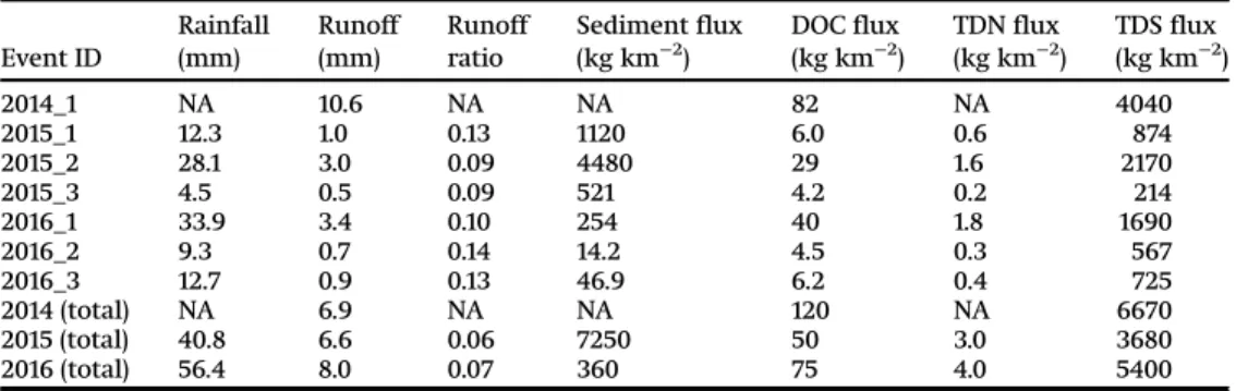
Table 1.Summary of total matter fluxes in the monitoring periods and the observed rainfall events and the according matter fluxes.

Event ID

Rainfall (mm)

Runoff (mm)

Runoff ratio

Sediment flux (kg km⁻²)

DOC flux (kg km⁻²)

TDN flux (kg km⁻²)

TDS flux (kg km⁻²)

2014_1 NA 10.6 NA NA 82 NA 4040

2015_1 12.3 1.0 0.13 1120 6.0 0.6 874

2015_2 28.1 3.0 0.09 4480 29 1.6 2170

2015_3 4.5 0.5 0.09 521 4.2 0.2 214

2016_1 33.9 3.4 0.10 254 40 1.8 1690

2016_2 9.3 0.7 0.14 14.2 4.5 0.3 567

2016_3 12.7 0.9 0.13 46.9 6.2 0.4 725

2014 (total) NA 6.9 NA NA 120 NA 6670

2015 (total) 40.8 6.6 0.06 7250 50 3.0 3680

2016 (total) 56.4 8.0 0.07 360 75 4.0 5400

Notes: Rainfall, runoff, runoff ratio, sediment, dissolved organic carbon (DOC), total dissolved nitrogen (TDN), and total dissolved solids (TDS) fluxes (in kg km⁻²) are reported for every rain event. NA, not available.

(7)

Flux estimates and statistics

To obtain flux estimates for parameterFp, mean runoff volumeQ during every time step twas multiplied with the concentration of the parameter [P]tat that time. The flux estimates are summed for the time interval of interesttn(Eq.1).

Fp=X^tⁿ

t0

ðQ×½PtÞ (1)

The mean runoff volumeQ for a time interval of interesttnis the mean of all discharge runoff values from half the interval before and aftertn(Eq.2). For example, if the interval is 6 h, the mean is computed from 3 h until 9 h.

Q=n⁻¹^tXⁿ⁺^tn²

t0−^tn2

Qt

(2)

Statistical tests used in this study were performed with RStudio (Version 1.0.153).

Normality of distributions was tested using the Shapiro–Wilk normality test. The student’s ttest was used to compare the means of parameters between for example different years. If the distribution was not normally distributed, the Wilcoxon Rank-Sum Test was applied. To test the correlation between two variables, the Pearson correlation coefficient was used.

Results

Meteorological conditions

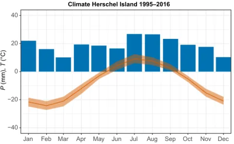
The mean annual air temperatures were−7.4 °C in 2014 and−6.3 °C in 2016 (Fig. 2) and therefore higher compared with the available climate record between 1995 and 2016 (−8.4 °C). The monthly air temperatures varied, with generally higher temperatures in the winter months compared with the long-term averages. The mean monthly air temperatures (1995–2016) for the monitoring months July and August were 9.0 and 7.3 °C, respectively.

Whereas the years of 2014 and 2015 showed mean monthly air temperatures of 9.1 and

Fig. 2. Climatic conditions retrieved from the automated weather station on Herschel Island between 1995 and 2016 including only months with no data gaps (Environment and Climate Change Canada 2018). The plot shows minimum, maximum, and mean temperaturesT(orange line and ribbon in °C) and precipitationP(blue in mm).

−40

−20 0 20 40

Jan Feb Mar Apr May Jun Jul Aug Sep Oct Nov Dec

P (mm), T (°C)

Climate Herschel Island 1995–2016

(8)

7.8 °C for July and 6.8 and 7.1 °C for August, the year of 2016 exhibited higher air temperatures in both months (9.4 and 7.7 °C). Snowmelt typically occurs in May. The mean monthly air temperatures for May 2014 and 2016 showed higher values (−1.2 and−0.1 °C) compared with the mean (−3.4 °C). Temperature data is unavailable for May 2015.

Rainfall for the monitoring period of 2015 (17 days) was 48 mm, and 47 mm for the monitoring period of 2016 (22 days). No precipitation data for Herschel Island or the closest climate stations is available for 2014. Due to this lack of consistent precipitation records, it was impossible to determine the climatic conditions comprehensively before the monitoring started.

Streamflow and EC

The major hydrological event during the year is the melting of snow in the spring. Peak flow reached 0.377 m³s⁻¹on 14 May 2016 (Fig. A3). Photos from the time-lapse camera show a change in the snow wetness and ponding 2 days prior to the initiation of flow (Appendix B).¹The high flow declined rapidly to 0.048 m³s⁻¹within 6 days, and a diel pattern was visible from week 21 onwards. A diel flow regime is characterized by higher stream discharge during daytime where remaining snow patches melt under the incoming solar radiation. The amount of precipitation during that time was not high enough to alter this diel flow pattern and appeared to have a minor contribution to the water flow in the steam.

As time progressed, the peak runoff during the day was shifted earlier; it occurred at 20:30 during week 21 and at 18:30 during week 24. Also, the amplitude decreased as snow left the catchment as runoff. From mid-June onwards (week 25), this pattern faded out indicating that melting of snow patches did no longer control the baseflow of the creek. EC rose expo- nentially from below 10μS cm⁻¹at the onset of snowmelt in 2016 to around 300μS cm⁻¹in mid June and it did not follow a diel pattern (Fig. A3). This period is termed nival recession.

From the end of June 2016 onwards, baseflow was controlled by rainfall events. We observed a total of seven rainfall events of different magnitudes in 2014, 2015, and 2016 (Fig. 3). Maximum flows recorded in the summer 2014–2016 were 0.024 m³s⁻¹in 2015, 0.044 m³s⁻¹in 2016, and 0.074 m³s⁻¹in 2014. This is substantially lower than flows that can be expected during spring freshet. In all 3 years of monitoring, the catchment responded quickly to the input of rain as indicated by linear rising hydrographs and the quick returns to baseflow conditions (Fig. 3). EC decreased with rising hydrographs and recovered thereafter. It reached maximum during the summer, up to 2000μS cm⁻¹as in July 2015. This period is referred to as baseflow/stormflow period. Rainfall to runoff ratios ranged between 0.09 and 0.14; 2015 being slightly less efficient in water export than 2016 (Table 1). As visible in the hydrographs throughout the years, baseflow rises with rainfall events (Fig. 3).

Transport of suspended sediment and organic matter

The transport of suspended sediment varied significantly (p<0.05) between both years of available summer data in 2015 and 2016 (Fig. 4;Table A1). The mean suspended sediment concentration was 1180 mg L⁻¹in 2015 and 28.2 mg L⁻¹in 2016, with minima of 167.5 mg L⁻¹ (2015) and 5.7 mg L⁻¹(2016), respectively (Table A2). Sediment and discharge hysteresis (Fig. 5) suggest a rapid initial mobilization of sediments during rainfall events followed by a exhaustion expressed as clockwise hysteresis loops. Peaks in sediment concentration were often reached before discharge peaked. The total sediment flux over the season amounted 7245 kg km⁻²in 2015 and 360 kg km⁻²in 2016. When looking at sediment export

1Supplementary material is available with the article through the journal Web site athttp://nrcresearchpress.com/doi/

suppl/10.1139/as-2018-0010.

(9)

in relation to water flux (Fig. 6a), event 2016-1 stands out because of its very low sediment flux. This result should be treated with caution, because the estimate is only based on available samples capturing the falling limb of the hydrograph. The high sediment pulse is likely to have occurred on the rising limb already.

POC values varied between 0.24 and 2.69 mg L⁻¹, with a mean of 0.75±0.58 mg L⁻¹. The carbon content of the suspended sediment ranged between 1.4% and 3.3% with a mean of 2.0±0.004%. Mean DOC concentrations were 11.1±0.8 mg L⁻¹in 2014, 8.8±2.1 mg L⁻¹in 2015, and 8.0±4.9 mg L⁻¹in 2016. The DOC concentrations between all years differed significantly (p<0.05;Table A1). Values for total dissolved nitrogen (TDN) ranged between 0.5 and 0.9 mg L⁻¹in 2015, and 0.5 mg L⁻¹, and 0.7 mg L⁻¹in 2016 (Table A2), being significantly

Fig. 3. Summary plot showing minimum, maximum and mean temperaturesT(orange line and ribbon in °C), precipitationPwhere available (blue in mm), discharge (m³s⁻¹), total dissolved solids (TDS), dissolved organic carbon (DOC), total dissolved nitrogen (TDN), and suspended sediment concentration (SSC) (all in mg L⁻¹) for the monitoring seasons 2014, 2015, and 2016. The rain events labels are indicated in the upper plots. Note that differences in sample treatment for DOC and TDN samples are indicated in the plots in grey. Values below the detection limit were set to the value of the detection limit.

(10)

different from each other (p<0.05). DOC shows a clear response to rainfall events, with increasing concentrations as flow increases (Fig. 5). DOC concentrations are commonly still rising after peak discharge; therefore, the hysteresis loop is counter-clockwise. The total DOC output was 123.5 kg km⁻²in 2014, 49.6 kg km⁻²in 2015, and 74.9 kg km⁻²in 2016. The TDN output was very low with 3.0 kg km⁻²in 2015 and 4.0 kg km⁻²in 2016 (Table 1). The relationship between water flux and output of DOC and TDN (Figs. 6b,6c) is very strong (R²_DOC=0.99;R²_TDN=0.99;p<0.05). Whereas we find a strong positive relationship (R²=0.99;p<0.05) between concentrations of POC and SSC (Fig. 7a), there is no clear relationship between SSC and DOC, POC and DOC, or SSC and TDS (Fig. 7).

Solute transport

The mean concentration of TDS—the summation of anions and cations—was 738± 134 mg L⁻¹in 2014, 553±247 mg L⁻¹in 2015, and 815±121 mg L⁻¹in 2016 (Table A2). The concentrations differed significantly between the years with the lowest average and greatest variability (between 365 and 1176 mg L⁻¹) observed in 2015. Decrease of TDS concentrations with increasing runoff during rainfall events was indicated by a clockwise hysteresis loop (Fig. 5). There is a strong positive relationship between water flux and TDS export (Fig. 6d) for all individual rainfall events (R²=0.99;p<0.05).

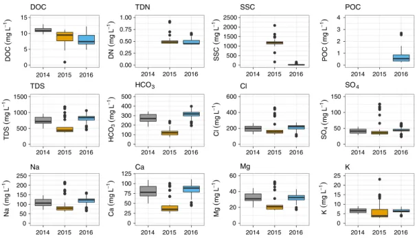
The major ions contributing to the sum of TDS were (highest to lowest) bicarbonate, chloride, sodium, calcium, sulfate, and magnesium (Fig. 4). All ions show a similar pattern as TDS with lower mean values in 2015, some of them being significant (Appendix A). We find that the outliers outside the fourth quartile occur just after the initiation of flow at the beginning of monitoring in 2015. Examining the hydrochemical facies in a piper diagram (Fig. 8) reveals that the composition of the water in 2015 differed from the other

Fig. 4. Boxplots showing hydrochemical concentrations of dissolved organic carbon (DOC), total dissolved nitrogen (TDN), suspended sediment concentration (SSC), particulate organic carbon (POC), total dissolved solids (TDS), and major ions at the outflow of Ice Creek West for 2014 (grey), 2015 (orange), and 2016 (blue). Note that values below the detection limit were set to the value of the detection limit. Boxplots for the remaining measured ions are found inFigure A4.

0 l

5 10 15

2014 2015 2016

DOC(mgL−1)(mgL−1) (mgL−1) (mgL−1) (mgL−1)(mgL−1)

(mgL−1) (mgL−1)

(mgL−1) (mgL−1) (mgL−1) (mgL−1)

DOC

ll ll

l ll

0.00 0.25 0.50 0.75 1.00

2014 2015 2016

DN

TDN

l

l ll ll

l llllll

0 500 1000 1500 2000 2500

2014 2015 2016

SSC

ll

0 1 2 3 4

2014 2015 2016

POC

ll l l l ll

l

l ll l l l

0 500 1000 1500

2014 2015 2016

TDS

ll l ll l l l

0 100 200 300 400 500

2014 2015 2016 HCO3

HCO3

ll l

l ll l l

l ll

0 200 400 600

2014 2015 2016

Cl

l l l

l l ll

l

l ll l l ll ll ll l ll

0 50 100 150

2014 2015 2016 SO4

SO4

l ll ll l

l

l ll l l ll

0 50 100 150 200 250

2014 2015 2016

Na

l ll ll l l l

ll l

0 25 50 75 100 125

2014 2015 2016

Ca

ll l

l ll l l

ll l

0 20 40 60

2014 2015 2016

Mg

l l

ll l

l ll

0 5 10 15 20 25

2014 2015 2016

K

(11)

2 years. Whereas in 2014 and 2016, the water type was mixed with no dominant facies, the composition shifts towards sodium chloride type in 2015. Compared with the other years, we find higher chloride concentrations and a slight decline in alkalinity in 2015. The total TDS output amounted 6670 kg km⁻²in 2014, 3680 kg km⁻²in 2015, and 5400 kg km⁻²in 2016 (Table 1).

Alluvial fan sampling

Results from sampling the outlets draining from the alluvial fan into the Beaufort Sea on 30 July 2016 are presented inTable 2, together with concentrations at the outflow from Ice Creek East and West at the same day. Suspended sediment concentrations were highly variable with 53.5 mg L⁻¹(POC: 4.0 mg L⁻¹) at location AF#2 and only 0.7 mg L⁻¹at location AF#5. Both locations are very close to each other on the eastern side of the alluvial fan (Fig. 1). DOC concentrations were very similar to the ones recorded at the outflow of the

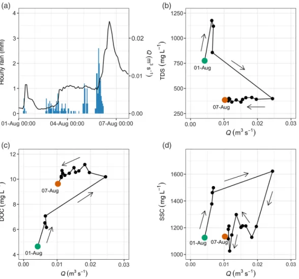
Fig. 5. Catchment response to 28.1 mm rainfall event 2015-2 (1–7 Aug.). (a) Rainfall and hydrograph response, (b) discharge–TDS hysteresis, (c) discharge–DOC hysteresis, and (d) discharge–SSC hysteresis. The hysteresis line follows every time step from the beginning (green dot) to the end (red dot) of the rainfall event, and the direction is indicated by the arrows. Hysteresis patterns for all recorded rain events can be found in the Figures A5andA6.

(12)

Ice Creek East and West (5.7 and 7.7 mg L⁻¹). They ranged between 4.7 mg L⁻¹at AF#6 and 8.1 mg L⁻¹at AF#3. TDN concentrations remained below the detection limit of 0.45 mg L⁻¹ for all sampling points. Concentrations of TDS were slightly lower after draining through the alluvial fan, ranging between 268.0 mg L⁻¹at AF#6 and 448.9 mg L⁻¹at AF#2.

Discussion

Hydrological response

The Ice Creek West watershed exhibits a typical nival flow regime, where snowmelt is the largest hydrological event of the year. Thawing of permafrost and melting of ground ice alone during the summer does not seem to generate substantial runoff. Therefore, summer baseflow is controlled by rainfall events and remains very low compared with the post nival recession. Watershed conditions prior to rainfall events have an effect on the runoff response. When monitoring started in 2015, there was no runoff at all in Ice Creek West, which points towards very dry conditions prior to that period. Although we do not have climate data to support this, there was presumably only little to no rain in the weeks prior to onset of monitoring. The 4.2 mm of rain during the 25th and 26th July did not generate flow. Only after the 8.1 mm rainfall event 3 days later, the catchment responded and the stream was activated. In contrast, rain events 2015-3 with 4.5 mm and 2016-3 with 12.7 mm occurred late in the season and did not show any discernible impact on the hydrograph. This shows that baseflow increases as more rainfall events occur during the late summer season. This finding is very typical for environments where water infiltra- tion is impeded by the permafrost table (Woo 2012). The hydrological response is directly

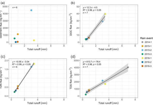
Fig. 6. Relation between total runoff and (a) sediment flux, (b) dissolved organic carbon (DOC) flux, (c) total dissolved nitrogen (TDN) flux, and (d) total dissolved solids (TDS) flux for all recorded rainfall events. All fluxes are reported in kg km⁻². The ribbon around the regression line indicates the standard error.

(13)

resulting in a sharply rising hydrograph, followed by an elongated falling limb. This is expected for a small catchment size of 1.4 km². The runoff ratios are in a similar range for all rainfall events (mean=0.11) indicating inefficient water routing and high water storage capacity in the watershed. If we assume a similar runoff ratio for 2014, we estimate the amount of rain to be roughly 76 mm based on the measured water flux. This would mean that the 2014 rain event was the greatest of all monitored years.Favaro and Lamoureux (2014)find a high range of runoff ratios between 0.001 and 0.84 in a 8.0 km²watershed (West River) at Cape Bounty, Melville Island in the High Arctic depending on the soil moisture conditions in the catchment.Carey et al. (2013)also find runoff ratios between 0.29 and 0.66 in a 7.6 km²alpine headwater stream (Granger Basin) in the discontinuous permafrost zone.

High runoff ratios indicate saturated antecedent conditions and thus, more efficient water routing. Projections for the Arctic show an increase of summer precipitation (Bintanja and Andry 2017), which would in turn, also lead to an increase in summer flow. Although the changes observed are not being significant, we find a decrease in drainage efficiency expressed through the runoff ratio later in the season (Table 1). This may reflect the deepening of the active layer, which increases the water storage capacity of the catchment.

Water quality and fluxes

DOC flux varies significantly between 124 kg km⁻² in 2014 and 49.6 kg km⁻²in 2015 (Table 1). The year of 2016 shows significantly higher DOC concentrations and flux (74.9 kg km⁻²) compared with 2015. These values need to be treated with caution as samples

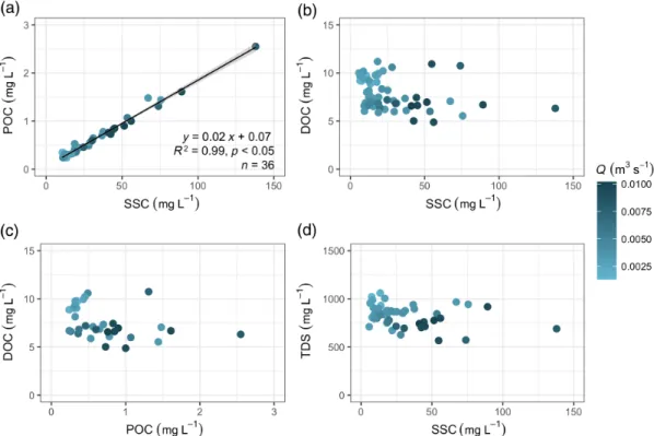
Fig. 7. Scatterplots showing the relation between (a) suspended sediment concentration (SSC) and particulate organic carbon (POC), (b) SSC and dissolved organic carbon (DOC), (c) POC and DOC, and (d) SSC and total dissolved solids (TDS) for the year of 2016. Concentrations are in mg L⁻¹. The colour of each point indicates the discharge (m³s⁻¹) at the time the sample was collected. The ribbon around the regression line in (a) indicates the standard error.

(14)

Fig. 8. Piper diagram showing the composition of major anions and cations at the outflow of Ice Creek West for 2014 (grey), 2015 (orange), and 2016 (blue).

Table 2.Concentrations of suspended sediment (SS), dissolved organic carbon (DOC), total dissolved nitrogen (TDN), total dissolved solids (TDS), and particulate organic carbon (POC) (all in mg L⁻¹) from Ice Creek West and the adjacent Ice Creek East as well as from outflows along the alluvial fan on 30 July 2016.

Location

SS (mg L⁻¹)

DOC (mg L⁻¹)

TDN (mg L⁻¹)

TDS (mg L⁻¹)

POC (mg L⁻¹)

Number of samples

Ice Creek East 3.8 5.7 <0.45 490.0 NA 1

Ice Creek West 12.7 7.7 <0.45 519.2 NA 1

AF#1 12.0 5.5 <0.45 332.8 NA 1

AF#2 53.5 6.6 <0.45 448.9 4.0 1

AF#3 25.1 8.1 <0.45 455.7 1.6 1

AF#4 3.2 6.7 <0.45 433.8 NA 1

AF#5 0.7 5.1 <0.45 416.2 NA 1

AF#6 5.8 4.7 <0.45 268.0 NA 1

Notes: NA, not available.

(15)

in 2015 and partly in 2016 were treated differently, and thus, may underestimate DOC concentration and flux (see“Suspended sediment and hydrochemistry”section for more details). We observe an increase of DOC export with increasing water flux (Fig. 6), which strongly suggests that DOC export is controlled by rainfall in our study site. Projected increase of discharge in the future (Bintanja and Andry 2017) may lead to higher DOC fluxes from the catchment.

Flux estimates for DOC have been reported for a number of locations across the Arctic (Table 3). For more adequate comparison, values from other studies were scaled down to 17 days of flux, i.e., the average monitoring period in this study. At Ice Creek West, we estimate the mean flux to be 82.7±30.7 kg km⁻²over all 3 years of monitoring (17 days in the summer). This value is higher than the DOC flux reported from the High Arctic, such as from Melville Island (1.6–25.7 kg km⁻²) byFouché et al. (2017) or Cornwallis Island (7.4 kg km⁻²) bySemkin et al. (2005). The availability of DOC is different between Low Arctic and High Arctic due to differences in vegetation cover. DOC fluxes are also reported from subarctic sites, such as Alaskan catchments with different permafrost coverage (18.8–43.5 kg km⁻²) byPetrone et al. (2006)and Granger Basin in the Yukon territory (28.6 kg km⁻²) byCarey (2003). These catchments drain areas of discontinuous permafrost and range below 10 km²in size. Flow pathways in those locations are possibly deeper, and may lead to less mobilization of DOC compared with our study site. The Mackenzie River, which is estimated to transport 50.2 kg km⁻²during a 17-day summer period, is a large Arctic River including areas of sporadic and without permafrost. Flux estimates from boreal watersheds in Sweden with no permafrost coverage (79.8–210.7 kg km⁻²) byLaudon et al. (2004)are much greater than those found in our study. Flux estimates for DOC (mean=1756.9 kg km⁻²) have also been provided byWeege (2016)for an outlet stream of a retrogressive thaw slump nearby our study site over two summer monitoring periods.

This value exceeds the other DOC yields greatly and might reflect the heavy disturbance associated with that location. Disturbances and thermokarst need to be taken into account when creating flux budgets.Holmes et al. (2012)provide the cumulative DOC flux for all six large Arctic Rivers, amounting 91.0 kg km⁻²for a 17-day summer period. Hence, our estimate is within the same range highlighting the relative importance of small watersheds in terms of DOC flux to the Arctic Ocean. Only rough estimates for the unmonitored circum-Arctic region are provided by (Holmes et al. 2012) assuming same aerial yields for the unmonitored watersheds. Comparing our Low Arctic flux estimates to other studies in the Subarctic and High Arctic highlights the spatial variability of fluxes across latitudes.

This will be of importance for future upscaling efforts. Besides riverine fluxes, coastal erosion including mobilization of ground ice might contribute to the DOC flux budget (Fritz et al. 2015).Tanski et al. (2016)estimated the DOC flux in ground ice mobilized through coastal erosion along the Yukon Coast to be 54 900±900 kg yr⁻¹. This shows that rivers and thaw streams are a much larger contributor of DOC to the coastal zone.

It is important to remember that this study is constrained to monitoring periods (on average 17 days) in the summers of 2014–2016. Comparing those values to the literature is very simplified and does not take into account any temporal variations from those sites (e.g., stormflow events). Further, as studies across the Arctic show, snowmelt as the major hydrological event, plays an important role for water quality and DOC flux in particular.

Petrone et al. (2006)find that 45% of DOC is transported during snowmelt,Laudon et al.

(2004)find 50%–68% in boreal Sweden, andFouché et al. (2017)reported 76%–99% for the same runoff period in the High Arctic. Our monitoring needs to be extended capturing the full hydrological year including the snowmelt period.

The suspended sediment (SS) export varies strongly between the years although the measured total runoff remains similar (6.6 mm in 2015 and 8.0 mm in 2016). The year of 2015 Arctic Science Downloaded from www.nrcresearchpress.com by BIBLIO DES WISSENSCHAFTSPARKS on 11/22/18 For personal use only.

(16)

Table 3.Annual, summer, and 17-days dissolved organic carbon (DOC) fluxes from different Arctic locations sorted by the 17-day DOC yield.

Catchment Study Area

Watershed (km²)

17-day DOC yield (kg km⁻²)

Summer DOC yield (kg yr⁻¹km⁻²)

Annual DOC yield (kg yr⁻¹km⁻²)

ALD Fouché et al. 2017 Melville Island, Nunavut 0.3 1.6 4 110

Caribou Fouché et al. 2017 Melville Island, Nunavut 0.3 1.9 5 420

Amituk Lake catchment Semkin et al. 2005 Cornwallis Island, Nunavut 26.5 7.4^a NA 160

CPCRW low Petrone et al. 2006 Alaska 5.3 18.8 152 430

Goose Fouché et al. 2017 Melville Island, Nunavut 0.2 24.4 57 870

Ptarmigan Fouché et al. 2017 Melville Island, Nunavut 0.2 25.7 60 260

CPCRW medium Petrone et al. 2006 Alaska 10 27.7 223 530

Granger Basin Carey 2003 Yukon Territory 6 28.6 541 1640

CPCRW high Petrone et al. 2006 Alaska 5.7 43.5 350 830

Mackenzie Holmes et al. 2012 Mackenzie River 1.68×10⁶ 50.2 363 820

Sörbacken Laudon et al. 2004 Northern Sweden 62 79.8 432 4800

Ice Creek West^b This Study^a Yukon Coast 1.4 82.7±30.7 NA NA

Västrabacken Laudon et al. 2004 Northern Sweden 0.1 99.8 540 3600

Lillan Laudon et al. 2004 Northern Sweden 21 118.3 640 6400

Stridbäcken Laudon et al. 2004 Northern Sweden 9 122.9 665 3500

Mellansjobacken Laudon et al. 2004 Northern Sweden 26 131.9 714 5100

Kallkalsbacken Laudon et al. 2004 Northern Sweden 0.5 180.3 976 6100

Kallkalstmyrn Laudon et al. 2004 Northern Sweden 0.2 210.7 1140 7600

Slump D Weege 2016 Yukon Coast 0.1 1756.9 NA NA

Arctic Rivers Holmes et al. 2012 Circum-Arctic 1.09×10⁷ 91.0 658 1670

Note:ALD, active layer detachment (catchment); CPCRW, Caribou Poker Creeks Research Watershed. This 17-day DOC yield was scaled down from summer DOC yields to make values from Ice Creek West comparable. Numbers from the literature were reduced to significant digits. NA, not available.

aNo summer estimate was available for this location, which is why the 17 d DOC yield is based on the entire year.

bMean of DOC fluxes recorded during the monitoring periods of the summers 2014, 2015, and 2016.

etal.765

PublishedbyNRCResearchPress

For personal use only.

(17)

shows a significantly higher sediment yield (7245 kg km⁻²compared with 360 kg km⁻²in 2016), which is most likely caused by a short-lived sediment supply. No major permafrost disturbances have been observed during that time, which leads to the hypothesis that the increase in sediment concentration is related to temporary channel and riverbank erosion.

The clockwise hysteresis loops observed in this study are consistent with findings byFavaro and Lamoureux (2014), who observe varying hysteresis patterns in the High Arctic depending on sediment availability. The sediment concentration is much lower in the summer of 2016, which implies, that all the available sediment has been flushed out of the system during the snowmelt period of 2016. Thus, the summer of 2016 did not seem to be influenced by the event anymore. This short-lived sediment mobilization differs from major disturbances such as active-layer detachments or retrogressive thaw slumps, which impact sediment delivery in streams over many seasons (Bowden et al. 2008;Frey and McClelland 2009;Lamoureux and Lafrenière 2009;Kokelj et al. 2013;Lamoureux and Lafrenière 2017).

Along with the increased sediment flux in 2015, we observe higher chloride concentrations and a slightly reduced alkalinity compared with the other years. The declining calcium carbonate source could indicate erosion of marine sediments, found on Herschel Island (Fritz et al. 2012). High TDS concentrations are known to correspond to groundwater contribution and may increase across the Arctic in the future (Frey and McClelland 2009). We find varying concentrations over the 3 years of monitoring. The concentration minima in 2015 could point towards greater surface water and less ground water contribution than in the other years.

We compare our SS flux estimates for 2015 and 2016 to other Arctic locations scaled to 17-day periods (Table 4) and find that our very low 2016 estimate is comparable to measurements at Boothia Peninsula in the High Arctic (100–300 kg km⁻²). Our high 2015 estimate exceeds values from Melville Island in the High Arctic (3200–6300 kg km⁻²) and also the Lena River (2300 kg km⁻²), but remains below fluxes from the Mackenzie River (20 300 kg km⁻²) and the disturbed Slump D nearby on Herschel Island (2.4×10⁶kg km⁻²). Transport of suspended sediment is highly variable across the Arctic region, and especially at our site, and between years. We do not find an increase of suspended sediment yield with decreasing watershed size as proposed byWalling (1983)orFryirs (2013)although this may be due to the fact that the values compiled here are covering a range of latitudes, geological settings and ecoregions, thus influencing this relationship. We also do not have other sites in the Low Arctic to compare our estimates to. Monitoring of small watersheds over several years is essential to capture interannual dynamics and to establish reliable flux estimates. The high 2015 estimate is similar to the sum of the six large Arctic Rivers (8470 kg km⁻²) underlining the importance of extended monitoring.

We find that 2.0% of the suspended sediment is composed of POC in our study site. This finding corresponds to the study at Cape Bounty in the High Canadian Arctic byLamoureux and Lafrenière (2014), who also find a linear relationship between POC and SSC (Table 4).

There, East River with an area of 11.6 km²shows a POC/SSC ratio of 2.2%, whereas West River (8.0 km²) shows a ratio of 2.0%. Also, ratios of the Ob and Mackenzie rivers (Holmes et al. 2002;Carrizo and Gustafsson 2011) are in a similar range as our study site. The melt- water stream draining Slump D nearby our study site has a mean POC to SSC ratio of 1.7%

for the summer monitoring periods. The ratio is the same for the large Arctic Rivers (without Yukon River). Contrary to the studies where annual fluxes are reported, our estimates are only based on the periods of stream monitoring in the summer. The POC to SSC ratio is unknown during snowmelt at our study site.

Local geomorphology may influence fluxes of DOC, TDS, and SS to the ocean. The Ice Creek watershed flows through an alluvial fan before draining into the Beaufort Sea, which is why we collected water samples along the fan outflows to investigate how concentrations Arctic Science Downloaded from www.nrcresearchpress.com by BIBLIO DES WISSENSCHAFTSPARKS on 11/22/18 For personal use only.