Organic matter incorporation into sea ice and potential matter release
into the nearshore zone of the southern Beaufort Sea, Canada
Kristoffer Nils Laux
A thesis presented for the degree of MASTER OF SCIENCE
Geology
Freie Universi¨ at Berlin Germany
Date of Submission: 29.09.2020
Supervisors: Dr. Michael Fritz - Alfred-Wegener-Institut Centre for Polar and Marine Research (AWI), Potsdam
Bennet Juhls - Freie Universit¨at Berlin
Reviewers: Prof. Dr. Liane Benning - Freie Universit¨at Berlin / Helmholtz Centre Potsdam - German Research Centre for Geosciences (GFZ)
Prof. Dr. Hugues Lantuit - Universit¨at Potsdam / Alfred-Wegener-Institut Centre for Polar and Marine Research (AWI), Potsdam
”Wir sehen in der Natur nie etwas als Einzelnheit, sondern wir sehen alles in Verbindung mit etwas anderem, das vor ihm, neben ihm, hinter ihm, unter ihm und ¨uber ihm sich befindet.”
Johann Wolfgang von Goethe
Zusammenfassung
Die globale Erw¨armung, die haupts¨achlich durch menschliche Einfl¨usse verursacht wird, hat in den letzten Jahrzehnten stark zugenommen. W¨ahrend die Erddurchschnittstemperatur im Zeitraum des gesamten letzten Jahrhunderts um etwa 0.8°C gestiegen ist, hat die Erw¨armung allein in den letzten 30 Jahren um 0.6°C zugenommen (GISTEMP, 2016; Lenssen et al., 2019).
Die Arktis hat sich mehr als doppelt so schnell erw¨armt wie der globale Durchschnitt (Serreze et al., 2009; Screen and Simmonds, 2010). Diese beschleunigte Erw¨armung hat dramatische Auswirkungen auf eine Vielzahl von Bereichen, einschließlich des Auftauens und Wiederge- frierens von Permafrostb¨oden. Die Landfl¨ache der n¨ordlichen Hemisphere ist mit etwa 23 Mil- lionen km2 zu fast ein Viertel von Permafrost beeinflusst. Wenn der Permafrost auftaut, vertieft sich die aktive Schicht und die j¨ahrliche Auftauphase der Permafrostb¨oden wird l¨anger. Infolge des Auftauens wird die damit verbundene Bodenwassermobilit¨at und die Erosionsrate erh¨oht und dadurch mehr Sedimente und gel¨oster organischer Kohlenstoff (DOC) in Seen, Fl¨ussen, Grundwasserfl¨ussen und K¨ustengew¨assern mobilisiert werden.
Meereiskerne und Wasser aus der darunter liegenden Wassers¨aule, wurden aus dem K¨ustengebiet des s¨udkanadischen Schelfes der Beaufort-See nahe der Insel Herschel - Qikiqtaruk entnommen, um den m¨oglichen Einbau organischer Stoffe, sowie die Freisetzung durch Winter-landfestes Meereis zu untersuchen. Meereis- und Wasserproben wurden an zwei sich kreuzenden Transekten entnommen, bevor die Schmelzsaison im Fr¨uhjahr 2019 begann. Analysen von gel¨ostem organ- ischem Kohlenstoff (DOC), farbiger gel¨oster organischer Substanz (CDOM), Salzgehalt, stabile Wasserisotopenverh¨altnisse sowie suspendierter Partikel (SPM) wurden durchgef¨uhrt, um Infor- mationen dar¨uber zu erhalten, wie und wieviel organisches Material w¨ahrend der Meereisbildung im Winter aufgenommen und w¨ahrend des Abschmelzens im Fr¨uhjahr freigesetzt wird.
Die gemessenen DOC-, CDOM- sowie SPM-Konzentration, sind im Vergleich zu Meereismessun- gen anderer Studien relativ niedrig. Isotopen- und Salzgehaltsmessungen zeigen an der S¨udseite von Transekt 1, dass die S¨ußwasser- und Flusseinfl¨usse im Winter abnehmen, was bedeutet, dass die S¨ußwasserquelle im Laufe des Winters versiegt und dadurch der Fluss als Quelle der organischen Substanz (OM) nahe liegt. Die Ergebnisse zeigen auch eine signifikante h¨ohere SPM-Konzentrationen in manchen k¨ustennahen Bereichen.
Die aus dieser Studie gewonnnen Daten zeigen, wie empfindlich die Regionen der Arktis und ihre Material- und Kohlenstofffl¨usse auf steigende Temperaturen reagieren, und deuten darauf hin, dass die K¨ustenerosion schon in Teilen der Wintersaison stattfinden kann.
Abstract
Global warming, mainly caused by human influences, has become much more severe in recent decades. While the average temperature of the Earth has increased of about 0.8°C over the time period of the entire last century, the temperature has increased by 0.6°C over only the past 30 years (GISTEMP, 2016; Lenssen et al., 2019). The Arctic region has warmed more than twice as fast as the global average (Serreze et al., 2009; Screen and Simmonds, 2010).
This accelerated heating has dramatic effects on a wide range of fields including the thawing and re-freezing processes of permafrost soils. Almost a quarter of the land area of the northern hemisphere is influenced by permafrost at around 23 million km2. When the permafrost thaws, the active layer deepens and the annual thawing phase of the permafrost soils becomes longer.
A result of the thawing is the associated soil water mobility and an increased rate of erosion, causing more sediment and dissolved organic carbon (DOC) to be deposited in lakes, rivers, groundwater fluxes and coastal waters.
In this work, sea ice cores and water from the water column below were sampled from the coastal area in the southern Canadian shelf of the Beaufort Sea, near Herschel Island - Qikiqtaruk, in order to investigate the possible incorporation of organic substances and the release from winter land-fast ice. The samples were collected from two intersecting transects, before the beginning of the melting season in spring 2019. Analyses of DOC, colored dissolved organic matter (CDOM), salinity, water isotope ratios as well as suspended particulate matter (SPM) were made, to gain information on how organic matter has been incorporated and released during the winter freeze up and through the season.
The measured DOC-, CDOM- and SPM-concentrations are relatively low compared to sea ice concentrations measured in other studies. Isotopes and salinity measurements show decreasing freshwater and river influences at the south side of transect 1 through the winter, meaning that the freshwater source petered out through the course of winter and through that giving indication of the river as the organic matter source. Results also showed a significantly higher SPM concentrations at the near shore north side of transect 1 and the west near shore side of transect 2.
The data obtained from this study show how sensitive the regions of the Arctic and their material- and carbon-fluxes react to rising temperatures and suggest that coastal erosion can occur already as early as part of the winter season.
Contents
Zusammenfassung i
Abstract ii
Selbstst¨andigkeitserkl¨arung / Statement of Authorship iii
1 Introduction 1
1.1 Scientific background . . . 1
1.2 Aims & objectives . . . 3
2 Study Area 4 2.1 The Arctic Ocean and the Beaufort Sea . . . 4
2.2 Shoreline and sea ice characteristics . . . 5
2.3 Study site - From Herschel Island to Kay Point . . . 7
3 Material & Methods 10 3.1 Field work . . . 10
3.2 Laboratory work . . . 11
3.2.1 Sample preparation . . . 11
3.2.2 Dissolved organic carbon & salinity . . . 12
3.2.3 Colored dissolved organic matter . . . 13
3.2.4 Stable water isotope geochemistry . . . 16
3.2.5 Suspended particulate matter . . . 16
4 Results 18 4.1 Overview . . . 18
4.2 Salinity . . . 19
4.2.1 Transect 1 . . . 20
4.2.2 Transect 2 . . . 21
4.3 Dissolved organic carbon . . . 22
4.3.1 Transect 1 . . . 24
4.3.2 Transect 2 . . . 25
4.4 Colored dissolved organic matter . . . 25
4.4.1 Transect 1 . . . 27
CONTENTS
4.4.2 Transect 2 . . . 28
4.5 Stable water - isotopes . . . 29
4.5.1 Transect 1 . . . 33
4.5.2 Transect 2 . . . 34
4.6 Suspended particulate matter . . . 35
4.6.1 Transect 1 . . . 37
4.6.2 Transect 2 . . . 38
5 Discussion 39 5.1 Ice formation and ice break-up . . . 39
5.2 Physico-chemical characteristics of sea ice . . . 42
5.3 Dissolved and particulate organic matter . . . 46
6 Conclusion 52
References 54
A Ice samples 63
B Water samples 68
List of Figures
1.1 Permafrost extent in 2003 compared to 2017. Continuous permafrost is defined as a continuous area with frozen material beneath the land surface, except for large bodies of water. None-continuous permafrost is broken up into separate areas and can either be discontinuous, isolated or sporadic. It is considered isolated if less than 10% of the surface has permafrost below, while sporadic means 10%-50%
of the surface has permafrost below, while discontinuous is considered 50%-90%.
From: Permafrost CCI, Obu et al, 2019 via the CEDA archive . . . 2 2.1 The Arctic Ocean on a global view with top five biggest Arctic rivers on water
discharge. Red map marker sets study area at Yukon coast within Beaufourt Sea.
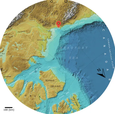
(Modified after ©Geographic Guide - Maps of World) . . . 5 2.2 Seafloor map of the Beaufort - Red map marker shows study area. (Modified
after ”THE INTERNATIONAL BATHYMETRIC CHART OF THE ARCTIC OCEAN” (IBCAO)) . . . 7 2.3 Land- and Pack ice environments. Landfast ice anchors at the shore until summer
break up. Stamukhi marks the border or outer rim of the landfast ice. In contrast to the landfast ice, the pack ice is free floating and, depending on in which region it is in, can last for several years. . . 8 2.4 Large image: Bathymetric map of the study area (Modified after: Federal publi-
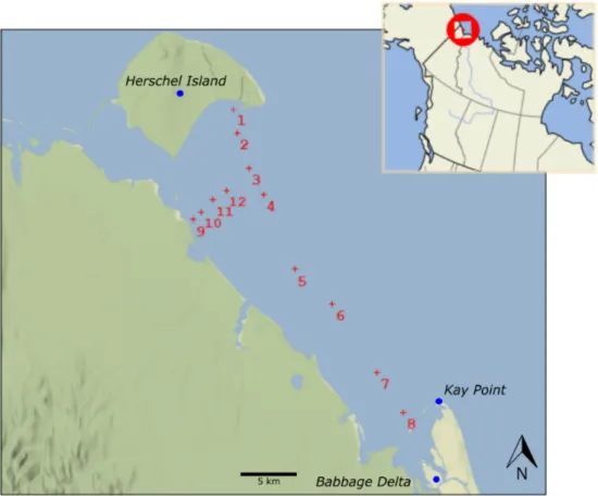
cations Inc: Nautical charts of the Beaufort Sea, 1998-2016); Small map (inset) showing study area and Mackenzie River Delta (Modified after: Google Earth 2020) 9 3.1 Sampling-Locations 2019. Red crosses marked with numbers indicate sampling
locations.
Transect 1: From 1 to 8. Transect 2: From 9 to 12 . . . 10 3.2 Sample preperation at the AWI Cold Chamber; Sea ice sawing, measuring and
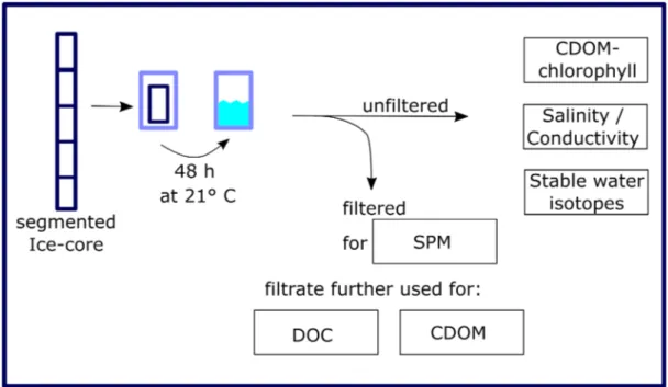
sampling . . . 12 3.3 Flowchart showing Sample-Workflow preparation for different parameters of anal-
yses. First ice core got sawed and segmented, each segment being brought to melt within 48 h. Afterwards is the melted sample being filtered or not filtered de- pending on the analysied parameter to be followed. . . 13
LIST OF FIGURES
3.4 General set up and method of a double beam spectrophotometer. Light is trans- mitted through monochromator where it gets filtered and then after passing the focus of the aperture, it is separated with mirrors into two beams to transmit
through the sample and reference sample to be lastly detected by the detector. . 14
3.5 Example showing the applied method to detect chlorophyll by distilling out the one significant chlorophyll peak within the red light wavelength (at around 675 nm). After Bennet Juhls. . . 15
4.1 Salinity of all twelve ice cores with relation to sampling depth. . . 19
4.2 Salinity of all twelve water samples with relation to sampling depth. . . 20
4.3 Salinity for ice cores along transect 1. From location 01 (0 m) close to Herschel Island until location 08 (36098 m) close to Kay Point. . . 20
4.4 Salinity for water samples along transect 1. From location 01 (0 m) close to Herschel Island until location 08 (36098 m) close to Kay Point. . . 21
4.5 Salinity for ice cores along transect 2. From location 09 (0 m) close to Yukon coast until location 12 (4611 m). . . 21
4.6 Salinity for water samples along transect 2. From location 09 (0 m) close to Yukon coast until location 12 (4611 m). . . 22
4.7 DOC concentrations of all twelve ice cores with relation to sampling depth. . . . 23
4.8 DOC concentrations of all twelve water samples with relation to sampling depth. 23 4.9 Salinity / DOC crossplot for ice cores. Each color and the corresponding number, stands for one specific ice core sample/location. . . 24
4.10 DOC concentration for ice cores and water samples along transect 1. From lo- cation 01 (0 m) close to Herschel Island till location 08 (36098 m) close to Kay Point . . . 24
4.11 DOC concentration for ice cores and water samples along transect 2. From loca- tion 09 (0 m) close to Yukon coast until location 12 (4611 m). . . 25
4.12 CDOM of all twelve ice cores with relation to sampling depth. . . 26
4.13 CDOM of all twelve water samples with relation to sampling depth. . . 26
4.14 CDOM / DOC crossplot of all twelve ice cores and water samples. . . 27
4.15 CDOM for ice cores and water samples along transect 1. From location 01 (0 m) close to Herschel Island till location 08 (36098 m) close to Kay Point. . . 27
4.16 SUVA for ice cores and water samples along transect 1. From location 01 (0 m) close to Herschel Island till location 08 (36098 m) close to Kay Point. . . 28
4.17 CDOM for ice cores and water samples along transect 2. From location 09 (0 m) close to Yukon coast until location 12 (4611 m). . . 28
4.18 SUVA for ice cores and water samples along transect 2. From location 09 (0 m) close to Yukon coast until location 12 (4611 m). . . 29
4.19 Depth overδ18Oof all twelve ice cores. Each color and the corresponding number, stands for one specific ice core sample / location. . . 30
4.20 Depths over δ18O of all twelve water samples. . . 31
LIST OF FIGURES
4.21 A co-isotopic plot of all twelve ice cores -δD againstδ18O in comparison with the GMWL (dark green) line. The red line shows the linear regression from water samples. The green line the linear regression of ice core samples. . . 31 4.22 δ18O / Salinity cross plot for ice cores and water- samples. . . 32 4.23 δ18O along transect 1 for ice core samples. From location 01 (0 m) close to
Herschel Island till location 08 (36098 m) close to Kay Point . . . 33 4.24 δ18Oalong transect 1 for water samples. From location 01 (0 m) close to Herschel
Island till location 08 (36098 m) close to Kay Point . . . 33 4.25 δ18Oalong transect 2 for ice core samples. From location 09 (0 m) close to Yukon
coast until location 12 (4611 m). . . 34 4.26 δ18O along transect 2 for water samples. From location 09 (0 m) close to Yukon
coast until location 12 (4611 m). . . 34 4.27 SPM concentrations of all twelve ice cores with relation to sampling depth. . . . 36 4.28 SPM concentrations of all twelve water samples with relation to sampling depth. 36 4.29 SPM concentrations for ice cores along transect 1. From location 01 (0 m) close
to Herschel Island till location 08 (36098 m) close to Kay Point . . . 37 4.30 SPM concentrations for water samples along transect 1. From location 01 (0 m)
close to Herschel Island till location 08 (36098 m) close to Kay Point . . . 37 4.31 SPM along transect 2 for ice core samples. From location 09 (0 m) close to Yukon
coast until location 12 (4611 m). . . 38 4.32 SPM along transect 2 for water samples. From location 09 (0 m) close to Yukon
coast until location 12 (4611 m). . . 38 5.1 Evolution of landfast ice throughout the year 2018-2019 between Herschel Island /
Qikiqtaruk and Kay Point at the Beaufort Shelf along the Yukon Coast, Canada.
07.10.2018 = One day before visible ice growing; 08.10.2018 = First major ice fields (Nilas) are starting to form along the coast (as landfast ice) and along Herschel Sill (Bedfast ice). By the end of October / beginning of November the ice shield has covered entire bay area. 15.04.2019 = Ice shield is still stable. Two weeks before core extraction. 08.06.2019 = First visible ice break up at summer.
Using Aqua/MODIS satellite provided by www.worldview.earthdata.nasa.gov . . 40 5.2 The Mackenzie River hydrology for the years 1973-1990 ( Watcr Survey of Canada).
The solid line shows the averagc daily rate of inflow whereas points show daily values. From R. Macdonald et al., 1998 . . . 41 5.3 The graph above shows Arctic sea ice extent as of October 2, 2019, along with
daily ice extent data for four previous years and the record low year (2012). The gray areas around the median line show the interquartile and interdecile ranges of the data collected between 1981 and 2010. From: National Snow and Ice Data Center, University of Colorado Boulder . . . 42 5.4 A portion of the phase diagram of NaCl-H2O for the ice and brine separation
during freezing. After W. F. Weeks and Ackley, 1986 . . . 43
LIST OF FIGURES
5.5 δ18Ovalues from HI-2 from Macdonald 1995 (left) vs. sample Ice-Loc.: 08 (right).
Similar low values found within the top section. . . 45 5.6 Ice-core sampling locations of this study (red crosses) including location 08 (blue
cross) and with sample HI-2 from Macdonald 1995 (green cross) . . . 46 5.7 CDOM absorption plots of unfiltered ice-core samples for chlorophyll analysis.
No significant peak between 500 to 600 nm can be made out. Left: total wave length range. Right: Close up of same plot with close up of wave length range from 400-800. . . 47 5.8 Ice core 08: Depths against DOC. Higher concentration within upper [0 - 0.20 m]
section of ice measured . . . 48 5.9 Conceptual model of POC pathways at the coast and in the nearshore zone. The
nearshore zone is divided in the resuspension zone (RZ) and the deposition zone (DZ).In the upper mixed layer, turbulent mixing by waves and currents is stronger at the surface and decreases with depth (blue arrow). During water column transport, OC can be remineralized and potentially released to the atmosphere as greenhouse gases (GHGs, red arrow) or reach the deposition zone and settle out to the sediment (green arrow). From Jong et al., 2020 . . . 49 5.10 Ice core 09: Depth against SPM. Higher concentration within upper [0 - 0.20 m]
section of ice measured . . . 50 5.11 Ice core 01, 07 and 08: Depth against SPM. 07 and 08 show a higher concentration
within upper section of core, indicating entrainment at the beginning of winter.
01 at the lower section, indicating entrainment at the end of winter. . . 51
List of Tables
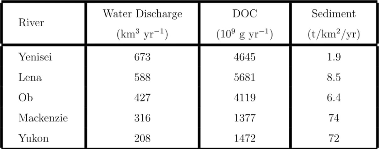
2.1 Water, DOC and sediment discharges of the top five rivers floating into the Arctic Ocean. After: R. M. Holmes et al., 2002; McClelland et al., 2016; R. M. Holmes et al., 2012 . . . 6 4.1 Mean values of ice core and complimentary water parameters. SD = Standard
deviation. . . 18 5.1 Salinity ranges for different water regimes. . . 44
List of Abbreviations
AO Arctic Ocean. 4, 7, 8, 14
AORB Arctic Ocean river basins. 4 AWI Alfred-Wegener-Institut. vi, 10–12
CDOM colored dissolved organic matter. ii, 11–15, 25, 47, 52 DOC dissolved organic carbon. ii, 11–13, 22, 25, 35, 47–49, 52 DOM dissolved organic matter. 1, 13, 15, 25, 47, 48, 53 GFZ German Research Center for Geosciences. 14 GMWL global meteoric water line. 29, 30, 46 LIS Laurentide Ice Sheet. 6, 8
OC organic carbon. 4
POC particulate organic carbon. 48
SPM suspended particulate matter. ii, 2, 11, 12, 35, 49, 52 SUVA specific ultra violet Absorbance. 15, 16, 48
TOC total organic carbon. 22 UV ultra violet. 13, 15
V-SMOW Vienna standard mean ocean water. 16
Chapter 1 Introduction
1.1 Scientific background
The oceans of the earth contain roughly the same amount of carbon, in the form of dissolved organic matter (DOM), as is present in our atmosphere in the form of carbon dioxide (CO2) (Hansell and Carlson, 2001). The mass of carbon found within the soils of the earth is higher than the masses of carbon in our atmosphere and in the entire living biomasses combined (Ciais et al., 2014). The main sources of terrigenous organic matter (OM) to the oceans are rivers, groundwater discharges, coastal erosion, sea ice inputs and aeolian material fluxes (Stein et al., 2004; Raymondet al., 1999). When global temperatures rise, profound geological effects can be triggered and the organic matter supply to the seas increase through a stronger river flux input, as well as eroding coastlines through thawing of permafrost (Fritz et al., 2017; Schuur et al., 2015; Freeman et al., 2001; Freemanet al., 2004; Frey and Smith, 2005). Since permafrost soil can only exist under temperature conditions which are below the freezing point, its existence is particularly endangered by rising air temperatures and changing climatic conditions and the eventual release of more greenhouse gases is expected (Christiansen et al., 2010; Vieira et al., 2010).
With the trend of rising temperatures over the past decades (Hansen et al., 2010), connected with greenhouse gases (Petitet al., 1999), humans bringing their emission each year to new level highs (Friedlingsteinet al., 2019), the projections for the future not look very good (Meehlet al., 2007; Collins et al., 2013; Slater et al., 2020). The prospects are especially bad for vulnerable regions of the Arctic and Antarctica (Serrezeet al., 2007; Maslaniket al., 2007; J. Comisoet al., 2007; Schaefer et al., 2014), which store a tremendous amount of carbon within their regions of permafrost. Recent studies calculated the global stock of soil organic carbon only within the permafrost to be around 1325 Pg (K¨ochy et al., 2015). For comparison, it is estimated that since 1850, with the beginning of the industrial revolution, about 440 ±20 Pg C was produced by humans and entered the atmosphere (Friedlingsteinet al., 2019).
Next to those regions of high elevations, the temperature within the atmosphere has not in- creased faster anywhere than in the polar regions (Pepin et al., 2015) and nowhere else can the results of the global warming be observed more obviously than at the polar regions with visible
CHAPTER 1. INTRODUCTION
Figure 1.1: Permafrost extent in 2003 compared to 2017. Continuous permafrost is defined as a continuous area with frozen material beneath the land surface, except for large bodies of water. None-continuous permafrost is broken up into separate areas and can either be discontinuous, isolated or sporadic. It is considered isolated if less than 10% of the surface has permafrost below, while sporadic means 10%-50% of the surface has permafrost below, while discontinuous is considered 50%-90%. From: Permafrost CCI, Obu et al, 2019 via the CEDA archive
thawing and vanishing of the permafrost, only withing the last decades (Fig.: 1.1).
Even if one assumes that the earth does not warm more than 2°C by 2100, the impact on per- mafrost would be catastrophic, with an estimated 40% loss (Chadburnet al., 2017).
Along with thawing other processes are likely to go hand in hand or be initiated, which will then further accelerate climate change. It can for example be assumed that, as a result of the thawing, microorganisms will increasingly begin to decompose the carbon that was previously stored in the permafrost soil and thereby release large quantities of the greenhouse gases, carbon dioxide and methane, into the atmosphere (Schaefer et al., 2014; Schuur et al., 2015). This in turn will affect other areas, such as the eco and hydro systems but also those of infrastructure (Bowden, 2010; Larsen and Fondahl, 2015; Radosavljevic et al., 2016; Hjortet al., 2018).
For many years now the Arctic, the ice and the carbon cycle has gained the focus of researchers from all fields (Stein et al., 2004) providing a better understanding and view on these highly important regions and matter.
There have been many improvements made in the field on gaining data by remote sensing from satellite pictures. For example, this is used to estimate the DOC concentration and fluxes in the waters for certain regions or oceans, by analysing the colored part of the dissolved organic matter, also known as CDOM (Matsuokaet al., 2017), providing e.g. insights about the source, the physiochemical as well as biological processes (Matsuoka et al., 2012). Others have used re- mote sensing technology to measure suspended particulate matter (SPM) concentrations within the waters (Li et al., 2015; Fettweis and Nechad, 2011), for tracking turbid river plumes or to
CHAPTER 1. INTRODUCTION
study the horizontal distribution, sinks and sources of SPM (Sathyendranath, 2000).
Isotopic data, on the other hand, yield important information about the origin and sources of different waters or can also be used for the reconstruction and determination of the paleoclimate (Dansgaard, 1964; Meyer et al., 2002). When combining isotopic analysis with other hydro- chemical properties, including CDOM and DOC, a more detailed and specific analysis on the origin and characteristics of ice and/or water samples can be achieved (Fritz et al., 2011; Juhls et al., 2020).
When it comes to in situ measurements, the focus of the research and expeditions for the polar regions has been narrowed down to those month of the year which make the region accessible to scientists. Due to the natural barriers given in the winter such as ice, cold temperatures and darkness (R. Macdonald et al., 1999), a sort of biased look through those brief warmer months has been created. The quantification of carbon fluxes from thawing permafrost, melting ground ice and coastal erosion and here in particular the role of winter sea ice in terms of incorporating, transporting and releasing carbon and particulates has still not been researched well enough to fully understand the carbon cycle and budget for this region (R. Macdonald et al., 1998; Fritz et al., 2015).
1.2 Aims & objectives
The aim of this thesis is to quantify the organic material in winter landfast ice with regard to the concentration and distribution within the ice cores regionally spanned over the two transects, and to analyze it with regard to its origin and potential release.
For this purpose, ice cores and the associated water samples from the water column below are examined for DOC, CDOM, salinity, water isotopes and the SPM entry. Not only are respective concentrations within the various ice cores quantified and analyzed, but also the concentrations in the regional distribution over the two transects are compared.
In advance, the following hypothesis was put forward:
Organic material from the thawing permafrost soils and the eroding coasts also accumulates in first year sea ice over the course of winter.
Chapter 2 Study Area
2.1 The Arctic Ocean and the Beaufort Sea
The study area with its two transects is located on the Canadian continental shelf along the Yukon Coast of the southern Beaufort Sea and is therefore part of the Arctic Ocean (AO) (Fig.
2.1).
The Arctic Ocean is connected to the Atlantic Ocean over a length of 1500 km and to the Pacific Ocean over a length of 85 km, via the Bering Strait. It holds an area of about 14x106 km2, which is almost the same size as Antarctica and with that, the AO is the smallest of the five major oceans on Earth.
Although the AO contains only 1% of the worlds ocean water, it receives 11% of the global runoff (Shiklomanov, 1993). Due to its position as the so called ”Arctic Ocean River Basin”
(AORB) (Lewis et al., 2000), it becomes a major player within the global water cycle.
The AO consists of the world’s largest shelf seas (Barents, Kara, Laptev, East Siberian, Chukchi, Beaufort and Lincoln Sea), which make up as much as 52.7 % of the entire area of the Arctic Ocean (Steinet al., 2004).
The continental shelf of the Beaufort Sea, compared to the others of the AO, is rather narrow (Fig. 2.1). Only close to the Mackenzie River mouth does it widen up to 145 km (Fig. 2.2).
These shelf regions of the Beaufort sea are subject to strong seasonal changes, during the summer being almost ice-free while they are almost entirely covered with ice in winter. The cold surface water layer of the Mackenzie Shelf has been found to have a low density compared to other shelf regions, due to the mixing with River runoff, sea ice melt and the influence of the low saline Pacific waters (Rudels et al., 1996).
Close to the coast the depth of the Beaufort Sea does not exceed more than 60 m, compared to the further offshore regions in the north, where the depth increases rapidly up to a few kilometers, forming the massive ”Canada Abyssal Plain” (Fig. 2.2).
The most important sources of freshwater and terrigenous OC, to the shelf seas and the AO, are large river and ground water discharges, coastal erosion, sea ice inputs and aeolian material fluxes (Rachold et al., 2004). The top five rivers in terms of annual volumetric water discharge to the AO are: Yenisei, Lena, Ob, Mackenzie and Yukon River respectively. The Yenisei, Lena
CHAPTER 2. STUDY AREA
Figure 2.1: The Arctic Ocean on a global view with top five biggest Arctic rivers on water discharge.
Red map marker sets study area at Yukon coast within Beaufourt Sea. (Modified after© Geographic Guide - Maps of World)
and Ob are located on the Russian continental shelf in Siberia, flowing into Kara- and Laptev Sea and the Mackenzie and Yukon River are located on the north American continental shelf flowing into the Beaufort and Bering Sea, respectively (Tab.: 2.1) (Fig. 2.1).
The mouth of the Mackenzie River in Northwest Territory (Canada) is on average 130 km away from the area from which the samples for this work were taken. (Fig. 2.2). It is the fourth largest river in terms of water discharge and has the highest sediment discharge to the Arctic Ocean (Rachold et al., 2004) (Tab.: 2.1).
The Beaufort Sea and the Mackenzie Delta host many small islands, and only a few bigger ones significantly extend out of the landscape towards the west of the delta, such as Herschel Island or ”Qikiqtaruk”, meaning “it is island” in the Inuvialuit language.
2.2 Shoreline and sea ice characteristics
34% of the world’s coasts consist of permafrost or are directly influenced by it (Lantuit et al., 2012). Permafrost soil is a soil, sediment or rock that remains at temperatures below the freezing point for at least two continues years. Permafrost terrain comprises a seasonally thawed active layer underlain by perennially frozen ground. It can vary in thickness and depths under the earth’s surface (Brown and Kupsch, 1974; Van Everdingen, 2005) and is therefore differentiated
CHAPTER 2. STUDY AREA
River Water Discharge
(km3 yr−1)
DOC (109 g yr−1)
Sediment (t/km2/yr)
Yenisei 673 4645 1.9
Lena 588 5681 8.5
Ob 427 4119 6.4
Mackenzie 316 1377 74
Yukon 208 1472 72
Table 2.1: Water, DOC and sediment discharges of the top five rivers floating into the Arctic Ocean.
After: R. M. Holmeset al., 2002; McClelland et al., 2016; R. M. Holmeset al., 2012
into different standard classifications:
• continuous permafrost (90 to 100% of the subsoil in a region is frozen)
• discontinuous permafrost (more than 50% of the subsoil of a region is frozen)
• sporadic permafrost (patchy distribution of the frozen subsoil) (Weise, 1983; French and Williams, 1976; Romanovskyet al., 2007).
Rampton, 1982 described the Yukon Coastal Plain, which is the extension of the Beaufort conti- nental shelf between the Mackenzie Delta and the Alaskan border, as an area mainly consisting of a thick layer of continues permafrost. It consists of Tertiary sandstones and shale, which are covered by a thin layer of uncosolidated sediments (Fritzet al., 2012) covered by the Laurentide Ice Sheet (LIS) during the Late Wisconsin.
In line with the Yukon coast, the coast of the study area is described as consisting of 65% un- lithified and 35% lithified with low cliffs (1 to 50 m) and mainly unconsolidated, frozen fine sand sediments (Lantuit et al., 2012). When these coasts are interacting with arctic marine as well as periglacial processes, they become an extremely dynamic and erosional environment (Harper, 1990; R. Macdonald et al., 1998) with erosion rates calculated of up to 2 m year−1 (Lantuit et al., 2012).
Within the area of this study are throughout the year and seasons, different kinds of sea ice being created, pushed in towards the coast and being released again offshore, to be partly subject of summer melt.
In general two different kinds of sea ice and zones of the nearshore sea ice environment can be distinguished. From coast to sea those are:
• Landfast ice, a largely undeformed sea ice that is ”fastened” / attached to the coastline, or to the sea floor (bedfast ice) and attaining a maximum thickness of about 2 m and a maximum extension offshore to the approximate 20-m isobath, with the stamukhi-zone (Reimnitz et al., 1978) being the natural last barrier before the polynya. With temper- atures dropping at around late October, landfast ice grows either in place from the sea
CHAPTER 2. STUDY AREA
Figure 2.2: Seafloor map of the Beaufort - Red map marker shows study area. (Modified after ”THE INTERNATIONAL BATHYMETRIC CHART OF THE ARCTIC OCEAN” (IBCAO))
water or by accumulation of drift or pack ice from the sea at the shore. Throughout the season this type of ice does not move, until melting begins.
• The stamukhi, a pebble ice field formed by ice convergence and collision of the offshore pack ice, extends downward, forming an inverted ‘dam’ of rubble ice plates (Fig. 2.3).
Beyond the stamukhi comes usually an area of flaw polynya.
• Flaw polynya is an open water area which can have a great extent or only be a narrow shear zone, before the area of pack ice.
• Seasonal and polar pack ice is the second type of sea ice. In contrast to the landfast ice it freely drifts on the AO (D. L. Forbes, 1981; W. Weeks, 2010).
2.3 Study site - From Herschel Island to Kay Point
The two transects at which the ice cores were drilled and the underlying water samples were taken span between Herschel Island (Qikiqtaruk), (69°35’ N, 139°5’ W) and Kay Point, (69°27’
N, 138°5’ W) (Fig. 3.1), a bay area located around 130 km west of the mouth of the Mackenzie River and 90 km east of the U.S. border to Alaska.
The Mackenzie River is the main fresh water and sediment source of the Canadian Beaufort
CHAPTER 2. STUDY AREA
Figure 2.3: Land- and Pack ice environments. Landfast ice anchors at the shore until summer break up. Stamukhi marks the border or outer rim of the landfast ice. In contrast to the landfast ice, the pack ice is free floating and, depending on in which region it is in, can last for several years.
Shelf (O’brien et al., 2006; R. M. Holmes et al., 2002) and as can be seen from Table 2.1, the Mackenzie River is, despite a lower water discharge in comparison to the other major rivers, an undisputed very large contributer of organic matter and suspended sediments for the AO and for large parts of the Beaufort Sea (Fichot et al., 2013). Thus, even though its mouth is at a greater distance, the Mackenzie River has a potential influence on the study area (R. Macdonald et al., 1998). However, this is very different from year to year and especially season to season.
The discharge peaks in June/July and falls sharply in winter (Woo and Thorne, 2003; Nghiem et al., 2014). However starting in mid to end of May, an already warmer water arrives at the river’s delta and begins to break up the sea ice within a few weeks (Mulligan et al., 2010).
In addition to Herschel Island and Kay Point, the bay is confined by the coastline of the Yukon coast and seaward by a narrow submerged ridge called Herschel Sill, which extends southeast from the eastern tip of Herschel Island until Kay Point and is a natural shallow bathymetric obstacle for water circulation in the basin and for fast ice development (Fig.: 2.4).
Near Kay Point the Babbage River flows into Phillips Bay (Fig.: 2.4), which is an Arctic River with a length of around 185 km, a catchment area of about 4750 km2 and an approximate water discharge of 11.3 m3s−1. The Babbage River carries source materials with a wide geological time spectrum, between Precambrian metaclastics over Palaeozoic and Mesozoic clastics and carbonates, until Quaternary glacial and non-glacial materials (D. Forbes, 1983).
Next to the Babbage River there are also other smaller rivers and creeks which flow into the study area, such as the Spring River and Roland creek (Fig.: 2.4), but like the Babbage River they run dry during the winter and have peak again during the month of snow melt (D. L.
Forbes, 1981).
The bathymetry between Herschel Island and Kay Point ranges between 5-10 m at Thetis and Phillips Bay and up to 80 m at Herschel Basin (Fig. 2.4), the basin as well as the aforementioned ridge right next to it (Herschel Sill) formed during the late Wisconsin period ( 21 to 11.3 cal ka BP) by dredging and carving of the LIS, on the dry-fallen shelf (Mackay, 1959; Fritz et al.,
CHAPTER 2. STUDY AREA
Figure 2.4: Large image: Bathymetric map of the study area (Modified after: Federal publications Inc: Nautical charts of the Beaufort Sea, 1998-2016); Small map (inset) showing study area and Mackenzie River Delta (Modified after: Google Earth 2020)
2012; Gowan et al., 2016).
During arctic winter, the months of October till May/June, landfast ice is a common feature between Herschel Island and Kay Point and forms a stable cover over most of the Mackenzie Shelf. Pack ice fields can be found about 80 km north of Herschel Island, drifting clockwise in a major offshore surface current along the Beaufort Sea, called the Beaufort Gyre. However, according to Dunton and Carmack, 2006 and Carmack and Macdonald, 2002 the currents effects do not affect the study area. Changing winds and season can, however, have the effect to push the pack ice towards the coast (Klock et al., 2001).
Chapter 3
Material & Methods
3.1 Field work
Fieldwork was performed and samples taken during an expedition led by the Alfred-Wegener- Institut (AWI) Helmholtz Centre for Polar and Marine Research (AWI) in Potsdam, Germany, as part of the EU funded project ”Nunataryk”, led by Hugues Lantuit. The samples used for this thesis were obtained between the 27th and 29th of April in 2019.
Sea ice and water samples from below ice were collected simultaneously at twelve locations, in two transects which were intersecting and perpendicular to each other (Fig. 3.1). The first
Figure 3.1: Sampling-Locations 2019. Red crosses marked with numbers indicate sampling locations.
Transect 1: From 1 to 8. Transect 2: From 9 to 12
CHAPTER 3. MATERIAL & METHODS
transect extends from Herschel Island (Location 01) coast across Herschel Basin towards Kay Point/Philips Bay (Location 08) which is the eastward limit of Herschel Basin and has a length of 36.1 km. The second transect runs from the Yukon mainland coast (Location 09) through Herschel Basin towards Herschel Sill (Location 12) with a lengths of 4.6 km.
Sample locations were visited with a skidoo and a sled. Due to safety reasons the limits of the fast ice edge were not crossed and therefore the station plan was adapted according to fast ice conditions. At each station coordinates were taken with a hand-held GPS. Snow depth was measured, before snow removal with a shovel for ice coring.
Ice cores were retrieved by an engine-powered Kovacs ice corer (Mark II) with an inner diameter of 9 cm and a core barrel length of 100 cm. Ice cores were drilled until sea water was reached.
Individual ice core pieces were cleaned with a knife, packed in tube foil and stored frozen in thermoboxes until further processing at the AWI cold lab in Potsdam.
The existing ice hole was enlarged with an engine-powered Jiffiy ice drill of about 30 cm diameter.
A CastwayCTD was used for water column profiling of temperature, conductivity and depth until the sea floor. Water samples were taken from surface water directly below the ice, from the middle of the water column and from bottom water with a 2.5 L Niskin bottle with manual trigger and a 2.5 L UWITEC water sampler depending on ice-hole conditions, water depth and trigger success. Water samples were filled up in 2 L Nalgene bottles and stored unfrozen in thermoboxes until further processing in the field camp.
Salinity, electrical conductivity and pH were measured on each sample directly in the field, using a WTW Multi 3430. Thirty milliliters were filled up in narrow-neck LDPE bottles for stable water isotopes and stored under cool (unfrozen) and dark conditions until further processing in the laboratory. Discrete amounts (about 1 L) of water was filtered through pre-weighed and pre-combusted 47 mm glass fibre filters (GF/F 0.7µm) for determining suspended particulate matter (SPM) concentrations. Filters were kept frozen until further processing in the lab.
Gum-free syringes with a syringe filter (23mm, GF/F 0.7µm) were used for DOC and CDOM filtration. DOC samples were filled up in clear glass vials with screwing lid and acidified with 1µL/ml HCl 30% suprapur, to prevent microbial conversion. CDOM samples were filled into 50 ml amber glass bottles. Both kinds of samples were stored in cool (unfrozen) and dark conditions until further processing at the laboratory.
3.2 Laboratory work
3.2.1 Sample preparation
The the sea ice-cores were cleaned with a knife and cut in half in the cold lab at about -10°C, using a Makita Band-Saw LB1200F, and one half was archived.
Half cores were split, using the same saw, into pieces ranging in sizes between 14 and 43 cm, to obtain enough volume for all analyses. The average length of the segments was 29 cm, depending on already existing cracks or general ice core length. Afterwards the cores were measured and put into labeled whirl-pak bags for further processing (Fig. 3.2). Preexisting, noticeable ice characteristics such as sediment inclusions or ice algae, were noted and the whirl-pak bags with
CHAPTER 3. MATERIAL & METHODS
Figure 3.2: Sample preperation at the AWI Cold Chamber; Sea ice sawing, measuring and sampling
the ice- samples were stored again into a freezer at -20°C before further processing.
In the hydrochemistry lab, ice samples were put into 2000 ml clean glass beakers, covered with pre-combusted aluminium foil (550°C), placed in the dark and stored at room temperature to melt. After 48 hours, sea ice samples had melted, and samples were homogenized by stirring with a glass stick. Approximately 90 ml of the melted sea ice was directly filled into narrow-neck bottles (each 30 ml) for stable isotope analysis, brown glass bottles (each 50 ml) for the CDOM- chlorophyll analysis and a miniature glass beaker (each 10 ml) for salinity/electrical conductivity analysis. The remaining meltwater was filtered through pre-weighted and pre-rinsed 47 mm 0.45 µm Sartorius cellulose acetate porefilters for SPM analysis, into a NalgeneT M filtration unit with receiver. The filtrate was split into brown glass bottles (each 50 ml) for CDOM analysis and glass-vials (each 20 ml) for DOC analysis. The DOC samples were acidified with 25 µL HCl suprapur (30 %). Figure 3.3 gives a brief overview on the main sample preparation processes and steps taken.
All sub-samples were stored in the dark at 4°C for further analysis described below. In total a number of 59 ice-core sub-segments out of the twelve ice-cores have been sampled. At the beginning, in the middle and at the end of the sample preperation, ”process blanks” were made (from Milli-Q Water) in order to check for any process errors.
3.2.2 Dissolved organic carbon & salinity
The dissolved organic carbon content of the samples was analyzed using high temperature cat- alytic oxidation (TOC-VCPH, Shimadzu). 20 ml of sample was placed into the auto-sampler of the analyzer. Before the actual measurement of the organic carbon was the inorganic car- bon, the inorganic carbon was removed by introducing sparge gas through the samples, along with hydrochloric acid which produced carbon dioxide (CO2). The remaining organic carbon
CHAPTER 3. MATERIAL & METHODS
Figure 3.3: Flowchart showing Sample-Workflow preparation for different parameters of analyses.
First ice core got sawed and segmented, each segment being brought to melt within 48 h.
Afterwards is the melted sample being filtered or not filtered depending on the analysied parameter to be followed.
was measured by catalytic combustion and measuring the CO2 concentration which converts into a DOC concentration. In order to keep the the accuracy of the measurement high, three replicate measurements of each sample were averaged, after every ten samples, a blank (Milli-Q water) and a standard were measured, using from eight different commercially available certified standards. Covering a range between 0.49 mg L-1 (DWNSVW-15) till up to 100 mg L-1 (Std.
US-QC). The results of standards provided an accuracy better than ±5h.
The salinity and electrical conductivity measurements were conducted with a Multilab 540 (WTW).
3.2.3 Colored dissolved organic matter
CDOM is a subset of DOM, which is coloured and thus shows absorption and fluorescence.
Whereas pure water absorbs light in longer wavelengths, CDOM absorbs light in short wave- lengths, ranging from 250 to 450 nm, and is therefore optically measurable by spectroscopy and fluorometry (Hoge et al., 1995). This ultra violet (UV) absorbance/fluoroscence acts as one of the primary regulators of light penetrating in the oceanic euphotic zone (Blough, 2002a) and hence also very likely acts as a strong contributor to the dependence of heat storage on depth, potentially directly effecting sea ice build-up (Matsuokaet al., 2011). Furthermore CDOM serves as an important food source for many organisms and bacteria. It also plays an important role in marine ecosystems through its feature of inhibiting light transmittance through the water column (Moran and Zepp, 1997; Blough, 2002b).
As CDOM is a subset of DOM it does positively correlate with it and can therefore be used as a supporting indicator for the general concentrations of DOM and DOC in the waters. The
CHAPTER 3. MATERIAL & METHODS
potential sources of CDOM are: soils, plants, wetlands, phytoplankton, zooplankton, sediments and generally all organic decaying products. In the Arctic the contribution of absorption by CDOM has been stated as remarkably high with over 76 % of the total nonwater absorbers (at 440 nm) (Matsuoka et al., 2007). This strong CDOM absorption in the Arctic Ocean is consis- tent with the already mentioned fact (Chapter: 2.1) that the AO receives the largest amount of freshwater relative to its volume.
For measuring the light absorption of CDOM different kinds of spectrophotometers exist.
A lamp inside the spectrophotometer provides a source of light. The beam of light strikes a diffraction monochromator, which functions like a prism by separating the light into its wave- lengths. This monochromator is rotated so that only a specific wavelength of light reaches the exit slit. Here, the light going out interacts with the sample water placed in a cuvet of specific lengths (Fig. 3.4). From this point, a detector measures the transmittance and absorbance com- ing through the sample. The detector senses the light being transmitted through the sample, and converts this information into a digital reading. For this work a double-beam spectropho- tometer was used, which works the same way as just described but additionally compares the light intensity between the light path of the sample cuvette and one path containing a cuvette with Milli-Q Water to reference the sample against it, and in this way all samples were blank corrected (Fig. 3.4).
Figure 3.4: General set up and method of a double beam spectrophotometer. Light is transmitted through monochromator where it gets filtered and then after passing the focus of the aperture, it is separated with mirrors into two beams to transmit through the sample and reference sample to be lastly detected by the detector.
For the work of this thesis the CDOM samples were collected in pre-rinsed 50 mL brown glass bottles that were stored in the dark at 4°C until analysis. αCDOM was measured at the at the German Research Center for Geosciences (GFZ), Potsdam, Germany using a LAMBDA 950 UV/Vis (PerkinElmer).
CHAPTER 3. MATERIAL & METHODS
The median absorbance (Aλ) of three replicate measurements was used to calculate theαCDOM(λ): αCDOM(λ)= 2.303∗Aλ
l (3.1)
where lis the path length, for which a 5 cm cuvette was used.
As mentioned before (Chapter: 3.2.1) two samples from the melted sea ice were taken. One filtered version for the standard CDOM analyses at 254 nm and one additional unfiltered sample.
The unfiltered sample was made in order to find out if there were any potential influences on the CDOM spectra by algae growth, measuring the chlorophyll concentration. In order to do so, a subtraction of wavelengths between the filtered and unfiltered sample pair was made, to get a clearer view on the final absorption graphs and to better carve out the chlorophyll peak in the red wavelengths region, explained in Figure 3.5 and the following equation.
α(λ) =α(λ)w +α(λ)phyt+αN AP(λ)+αCDOM(λ) (3.2) where subscriptions α, λ, w, phyt, N AP and CDOM indicate: Absorption coefficient, Wave- length, Water, phytoplankton, non-algal particles, and colored dissolved organic matter, respec- tively.
Figure 3.5: Example showing the applied method to detect chlorophyll by distilling out the one significant chlorophyll peak within the red light wavelength (at around 675 nm). After Bennet Juhls.
The absorption coefficient in this equation (Equat. 3.2) is expressed as the sum of the absorption coefficients of the different groups of components within the unfiltered samples. The magnitude of the absorption coefficient varies linearly with the concentration of the absorbing materials.
The absorbance at 254 nm has been shown to be strongly correlated with the hydrophobic organic acid fraction of DOM (Spencer et al. 2012) and is a useful proxy for DOM aromatic content (Weishaaret al., 2003) and molecular weight (Chowdhury, 2013). For that reason it was chosen to also use absorbance at 254 nm on CDOM analysis and to calculate for the specific UV absorbance SUVA (Weishaar et al., 2003). Dissolved organic matter originating from a terrestrial source has a higher aromatic carbon content than autochthonous or altered DOM.
This fact is used with the SUVA parameter to search for substances derived from plant or soil organic matter. Since aromtatic substances absorb light more strongly in the UV spectrum, a higher value of SUVA can give indication about increased aromatic content from allochthonous sources, vice versa for lower SUVA values (Battin, 1998).
CHAPTER 3. MATERIAL & METHODS
SUVA values were calculated using the equation:
SU V A= (A254/L)/[DOC] (3.3)
where A254 is the absorbance at 254 nm measured, L is the optical pathlength (0.05 m) and DOC is the dissolved organic carbon concentration in mg/L.
3.2.4 Stable water isotope geochemistry
Oxygen and hydrogen, the elements which bound together to water, in addition to their main and most common stable isotopes (H216O) also exist in other less common isotopes, as such there are: 17O, 18O for oxygen and 1H and D (Deuterium) / 2H for hydrogen. Between these isotopes there is a wide range of combinations and abundances found, which varies in the order of hundreds per mil (Jouzel, 2003).
As water is distributed and redistributed in regions that differ by depth, heights, longitude and latitude, it transitions between phases over and over again. Those phase transitions are strongly temperature dependent and influence the isotopic ratio and signal. These repetitive cycles are called the hydrological cycles (Criss et al., 1999) which lay the foundation of the fractionation processes by stable water isotopes and eventually lead to their characteristic isotopic signatures, formed within different water reservoirs.
Based on these fundamental processes the following method has been applied for this thesis, to be able to assign and differentiate between water sources.
A brief explanation of the basis for this method is as follows. Lighter water isotopes evaporate more easily and accumulate through rain again in freshwater sources such as rivers or lakes, whereas heavier isotopes remain in their regimes, such as snow covers or ocean waters.
The obtained values given in relation to the Vienna standard mean ocean water (V-SMOW), the most widely used standard (defined to be exactly 0 h) of the mean ocean water which approximates the bulk isotopic composition of the present-day global ocean reservoirs (Craig, 1961).
Measurements were conducted at the laboratory facility for stable isotopes at AWI Potsdam using a Finnigan MAT Delta-S mass spectrometer equipped with calibration units for the online determination of hydrogen and oxygen isotopic composition. The data is given as δD andδ18O values, the δ as the per mille difference to standard V-SMOW.
The measurement accuracy for hydrogen and oxygen isotopes was better than ±0.8h forδ18O and ±0.1h forδD, respectively (Meyeret al., 2000).
3.2.5 Suspended particulate matter
Suspended particulates of matter are microscopic particles of solid or liquid matter suspended in the air or in natural waters. They are commonly defined in relation to a minimum diameter, depending on the pore size of filters used to accumulate them (Loring and Rantala, 1992).
As already mentioned in chapter 3.2.1, in order to filtrate the suspended particulate matters out of the melted sea ice sample, 47 mm 0.45 µm Sartorius cellulose acetate, porefilters were used
CHAPTER 3. MATERIAL & METHODS
in combination with a NalgeneT M reusable filter holders with receiver. Before filtration, each filter was dried at 50°C in an oven, taken out, cooled down to room temperature in a dessicator and weighted directly afterwards to receive a pure filter weight, using a high precision scale by Mettler Toledo with an accuracy of 0,001 g. The filters were then placed into the filter holder and a little amount of the sample water (∼20 ml) used to pre-rinse the filters and to clean of any eventual carbon contents. Afterwards the entire sample was filtered, using an electric vacuum pump. The volumes of the sample waters were noted, for further calculation of the SPM concentrations. After the filtration was completed, the filters were carefully removed from the filter holder, placed in an individual numbered, precleaned petri dish and then put back in the sample-oven for a minimum of 48 hours to dry. After drying the samples were again taken out of the sample-oven, cooled to room temperature in a dessicator and then weighted again, using the same scale as before and receiving the filter weight with particles (≥0.45µm).
Chapter 4 Results
4.1 Overview
In the following chapter the data will be presented resulting from the twelve sea ice cores (YC19- ICE-01 - 12) and complimentary water samples (YC19-WAT-01 - 12) taken from below, on the expedition mentioned in chapter 2.1.
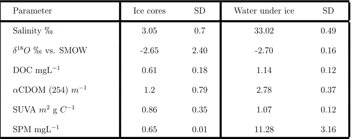
As a first overview, table 4.1 provides the mean values of all measured and calculated parameters of ice core and water samples, from all twelve locations combined and can be used to compare the relative differences between the different samples, locations and types.
Parameter Ice cores SD Water under ice SD
Salinity h 3.05 0.7 33.02 0.49
δ18O h vs. SMOW -2.65 2.40 -2.70 0.16
DOC mgL−1 0.61 0.18 1.14 0.12
αCDOM (254) m−1 1.2 0.79 2.78 0.37
SUVA m2 gC−1 0.86 0.35 1.07 0.12
SPM mgL−1 0.65 0.01 11.28 3.16
Table 4.1: Mean values of ice core and complimentary water parameters. SD = Standard deviation.
Figure 3.1 shows that the samples were taken in two intersecting transects, in order to see if regional differences in the organic matter incorporation exist. All data including those not shown here, can be found in the appendix.
The different ice core lengths range between 120 cm (ICE-07) and 186 cm (ICE-05) with a mean length of 146 cm. The complimentary water samples to the ice cores, were taken at the same locations as each sample. At each location three samples were taken from the water column, at top, mid and bottom. Depending on the bathymetry (Fig.: 2.4) the depths ranged between a minimum of 5.77 until a maximum depth of 59.77 m.
CHAPTER 4. RESULTS
4.2 Salinity
Measurement of salinity gives an indication about the salt or ionic content of seawater and can give information about the water regime, whether or not the sample water has a high or low freshwater content as well as about the structure of the water column. Salinity measurements in sea ice can also reveal information about its growth process.
Generally, when comparing ice cores with water samples, there is to note that the relative range of concentrations is a bit wider for the ice cores than it is with the different water samples. The lowest salinity concentration measured within the ice core was 1.2 hand the highest 4.6 h. This compares to 31.96 hand 34.68 hrespectively for the water samples. The average salinity value for the ice cores lays at 3.05 hand for the water samples 33.01 h.
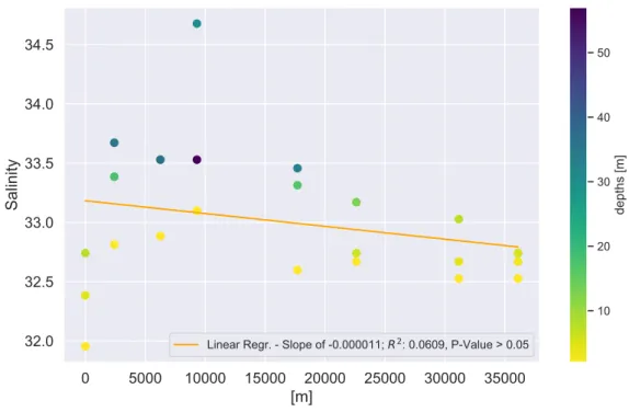
The overall salinity level of all cores plotted over the depths, shows a slight trend towards a higher concentration of salt in the upper sections, closer to the surface (Fig. 4.1), yet with a R2 of 0.02 and a p-value of >0.05 is the correlation very low. For the water samples a better correlation is observed and the opposite is true, lower concentration at the top and higher concentration in the lower section (Fig. 4.2). Along transect 1 the salinity concentrations for both water and sea-ice samples decrease towards Kay Point, indicating more freshwater input (Fig. 4.3; 4.4). Transect 2 does not show, for the ice cores nor for the water samples (Fig.: 4.5;
4.6), a significant trend (p >0.05), indicating only sea water within its range.
6DOLQLW\
'HSWKV>P@
/LQHDU5HJU6ORSHRI
R
239DOXH!Figure 4.1: Salinity of all twelve ice cores with relation to sampling depth.
CHAPTER 4. RESULTS
6DOLQLW\
'HSWKV>P@
/LQHDU5HJU6ORSHRIR239DOXH
Figure 4.2: Salinity of all twelve water samples with relation to sampling depth.
4.2.1 Transect 1
>P@
6DOLQLW\
/LQHDU5HJU6ORSHRIR239DOXH
Figure 4.3: Salinity for ice cores along transect 1. From location 01 (0 m) close to Herschel Island until location 08 (36098 m) close to Kay Point.
CHAPTER 4. RESULTS
>P@
6DOLQLW\
/LQHDU5HJU6ORSHRIR239DOXH!
GHSWKV>P@
Figure 4.4: Salinity for water samples along transect 1. From location 01 (0 m) close to Herschel Island until location 08 (36098 m) close to Kay Point.
4.2.2 Transect 2
>P@
6DOLQLW\>@
/LQHDU5HJU6ORSHRIR239DOXH!
Figure 4.5: Salinity for ice cores along transect 2. From location 09 (0 m) close to Yukon coast until location 12 (4611 m).
CHAPTER 4. RESULTS
>P@
6DOLQLW\>@
/LQHDU5HJU6ORSHRIR239DOXH!
GHSWKV>P@
Figure 4.6: Salinity for water samples along transect 2. From location 09 (0 m) close to Yukon coast until location 12 (4611 m).
4.3 Dissolved organic carbon
As one of the main analysis for this study does the dissolved organic carbon analysis contribute to the quantification of the sea ice cores and water samples taken. DOC is the fraction of total organic carbon (TOC), that passes through a filter size range between 0.22 and 0.7 µm. DOC in the coastal waters and in sea ice originates from various autochthonous and allochthonous sources such as dead organic matter, including plants and animals.
The lowest DOC concentration measured within the ice core was 0.36 and the highest 1.43 [mgL−1]. 1.02 and 1.68 [mgL−1] respectively for the water samples. The average DOC value for the ice cores lays at 0.61 [mgL−1] and for the water samples a twofold higher mean concentrations is observed 1.14 [mgL−1].
When comparing the depths of all ice cores against their DOC concentrations, no significant trend or concentration towards a certain depth was found (R2: 0.00, p > 0.05). The DOC concentration seems equally distributed (Fig. 4.7). In contrast, the water samples show a stronger trend of higher concentrations towards upper water-levels (Fig. 4.8).
When comparing the ice cores with the water samples from below along the transect 1 (Fig.:
4.10) it is noticeable that water and the ice show opposite trends, for the water samples an increase towards Herschel Island and for the ice cores an increase towards Kay Point, with the latter stronger than the water samples. Both show higher concentrations than their respective mean, close to the respective coast (at 0 m and 36098 m).
The crossplot between DOC and Salinity (Fig.: 4.9) for the ice cores shows no strong correlation
CHAPTER 4. RESULTS
(R2: 0.01, p > 0.05). Some ice cores cluster within a certain area (indicated by the different colors), for example 08 or 10.
Transect 2 does not show, neither for the ice cores nor for the water samples (4.11) a significant trend (R2: 0.01, p >0.05), indicating only sea water within its range.
'2&>PJ/@
'HSWKV>P@
/LQHDU5HJU6ORSHRIR239DOXH!
Figure 4.7: DOC concentrations of all twelve ice cores with relation to sampling depth.
'2&>PJ/@
'HSWKV>P@
/LQHDU5HJU6ORSHRIR239DOXH
Figure 4.8: DOC concentrations of all twelve water samples with relation to sampling depth.
CHAPTER 4. RESULTS
6DOLQLW\
'2&>PJ/@
/LQHDU5HJU6ORSHRIR239DOXH!
,&(
Figure 4.9: Salinity / DOC crossplot for ice cores. Each color and the corresponding number, stands for one specific ice core sample/location.
4.3.1 Transect 1
'LVWDQFHV>P@
'2&>PJ/@
,&(
:DWHU
/LQHDU5HJU6ORSHRIR239DOXH!
/LQHDU5HJU6ORSHRIR239DOXH
Figure 4.10: DOC concentration for ice cores and water samples along transect 1. From location 01 (0 m) close to Herschel Island till location 08 (36098 m) close to Kay Point
CHAPTER 4. RESULTS
4.3.2 Transect 2
'LVWDQFHV>P@
'2&>PJ/@
,&(
:DWHU
/LQHDU5HJU6ORSHRIR239DOXH!
/LQHDU5HJU6ORSHRIR239DOXH!
Figure 4.11: DOC concentration for ice cores and water samples along transect 2. From location 09 (0 m) close to Yukon coast until location 12 (4611 m).
4.4 Colored dissolved organic matter
Colored dissolved organic matter CDOM is the optically measurable component of DOM within water.
Hence CDOM is a subset of DOC the two quantities are strongly correlated within the ice and the waters (Fig.: 4.14). Also the general trend over the transect 1 (Fig. 4.15) as well as the concentration distribution over the depths (Fig. 4.12; 4.13) very much align, althoguh a slightly higher concentration within the upper sections is apparent, when compared to the DOC (Fig.
4.7; 4.8). The lowestαCDOM (254) measured within the ice core was 0.85 and the highest 5.76 [m−1]. The highest and lowest were 2.38 and 4.20 [m−1] respectively for the water samples. The average αCDOM (254) value for the ice cores lays at 1.20 [m−1] and for the water samples 2.78 [m−1].
The SUVA along the transect 1 plot (Fig.: 4.16) follows generally the trends of DOC and CDOM.
Peaks for the ice cores close to Kay Point at location 08 (36098 m) and for the water samples near the Herschel Island shore, are shown.
The same homogeneous distribution as previously described for the DOC and CDOM distribu- tions over transect 2 is also found here for SUVA on transect 2 (Fig.: 4.17; 4.18).
CHAPTER 4. RESULTS
a
254>m
1@
'HSWKV>P@
/LQHDU5HJU6ORSHRI
R
239DOXH!Figure 4.12: CDOM of all twelve ice cores with relation to sampling depth.
a
254>m
1@
'HSWKV>P@
/LQHDU5HJU6ORSHRIR239DOXH!
Figure 4.13: CDOM of all twelve water samples with relation to sampling depth.