Bacterial colonization and vertical distribution of marine gel particles (TEP and CSP) in the Arctic Fram Strait
Kathrin Busch1, Sonja Endres1, Morten Iversen2, Jan Michels1, Eva-Maria Nöthig3and Anja Engel1*
1Department of Marine Biogeochemistry/Biological Oceanography, GEOMAR Helmholtz Centre for Ocean Research Kiel, Kiel, Germany
²Department Deep Sea Ecology and Technology/SEAPUMP, Alfred Wegener Institute Helmholtz Centre for Polar and Marine Research, Bremerhaven, Germany
3Department Polar Biological Oceanography, Alfred Wegener Institute Helmholtz Centre for Polar and Marine Research, Bremerhaven, Germany
Supplementary material
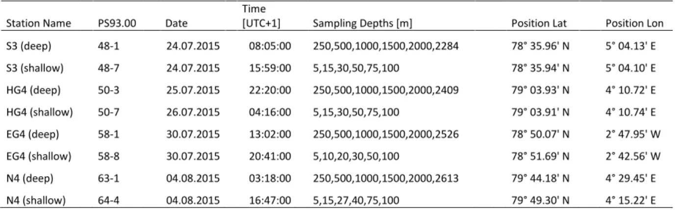
Table S1 Station list including the coordinate positions and exact sampling depths for all sampled stations.
Station Name PS93.00 Date Time
[UTC+1] Sampling Depths [m] Position Lat Position Lon S3 (deep) 48-1 24.07.2015 08:05:00 250,500,1000,1500,2000,2284 78° 35.96' N 5° 04.13' E S3 (shallow) 48-7 24.07.2015 15:59:00 5,15,30,50,75,100 78° 35.94' N 5° 04.10' E HG4 (deep) 50-3 25.07.2015 22:20:00 250,500,1000,1500,2000,2409 79° 03.93' N 4° 10.72' E HG4 (shallow) 50-7 26.07.2015 04:16:00 5,15,30,50,75,100 79° 03.91' N 4° 10.74' E EG4 (deep) 58-1 30.07.2015 13:02:00 250,500,1000,1500,2000,2526 78° 50.07' N 2° 47.95' W EG4 (shallow) 58-8 30.07.2015 20:41:00 5,10,20,30,50,100 78° 51.69' N 2° 42.56' W N4 (deep) 63-1 04.08.2015 03:18:00 250,500,1000,1500,2000,2613 79° 44.18' N 4° 29.45' E N4 (shallow) 64-4 04.08.2015 16:47:00 5,15,27,40,75,100 79° 49.30' N 4° 15.22' E
S2 Exemplary micrographs. Upper pannel : TEP stained with Alcian Blue (left) and associated bacteria stained with DAPI (right). Lower pannel: CSP stained with Coomassie Brilliant Blue G (left) and associated bacteria stained with DAPI (right). Scale bars in all micrographs represent 10µm (left micrographs: bright-field microscopy; right micrographs:
wide-field fluorescence microscopy).
S3 Size frequency distributions for both gel particle classes (CSP and TEP) at the different stations on a log-log scale. In each plot the frequencies (which were extrapolated to [mL-1 µm-1]) of the different ESD size classes (dp) are plotted for both replicates and all 12 depths.
The first size class represents 1µm. Size classes covered always a range of 0.5µm each.
Although the maximal particle sizes, which were only measured occasionally, are also depicted in the plot (white area), only the size range covered by the grey shaded area was taken to fit the regression. Resulting regression lines (dN/d[dp]=kdpδ
) are indicated by grey lines and their calculated coefficients δ are shown in Table S7.
S4 Detailed description of the digital image processing to determine total abundances of bacteria per gel particle (area).
The workflow of the developed image analysis procedure to determine total abundances of bacteria per gel particle (area) will be described in the following for one exemplary filter spot (i.e. for one of the ten filter sectors captured per filter).
In a first step both micrographs -taken from the same filter spot- were simultaneously openend in the image analysis software Image J (version 1.48). For the bright-field micrograph, depicting stained gel particles, the red color channel was chosen. For the wide- field fluorescence micrograph, depicting bacterial signals, the blue channel was chosen. On the bright-field micrograph the particles were thresholded and the particle parameters (routinously area, perimeter, major, minor and feret) were measured and recorded by the software. Afterwards, continuing in Image J, a bounding rectangle (i.e. the smallest rectangle enclosing the particle) was created around each thresholded particle in the bright-field micrographs. For these bounding rectangles the x- and y-coordinates of the upper left corner (x1 and y1), as well as the height and the width, were recorded into a text file (after applying a coordinate system with an inverse y-axis on the micrographs). Subsequently the perimeter(s) of all thresholded particle(s) were selected on the bright-field micrograph and the selection was transferred to the corresponding wide-field fluorescence micrograph. On the wide-field fluorescence micrograph, all maxima (i.e. the most intensely DAPI stained spots) were detected within the selection. Those maxima were counted and considered to represent the number of all bacterial cells attached to the thresholded particles, as the two pictures show exactly the same filter position. Before counting the maxima, an individual noise tolerance level was set to verify that the maxima supposed by the software correspond to real bacterial signals, and to furthermore account for varying signal intensities on the analysed micrographs.
Besides counting the maxima, also the centroids (which are the center points of the DAPI signals) were determined and the coordinates of those points (X and Y) were recorded into a second text file. Then, using MATLAB (version R2011a), the information of the two micrographs was combined. Both priorly produced text files were loaded and the second x- and y- coordinates (x2 and y2) of the bounding rectangles were calculated. Then it was tested for each bounding rectangle and all DAPI signal centroids, whether the X- and Y- coordinates of the DAPI signals' centroid were falling into a bounding rectangles coordinate range (i.e. if:
x1< X >x2 and y1< Y >y2). If this was true, a 1 was written into a set up matrix. If the condition did not apply, a 0 was printed at the according place into the matrix. After checking all possible combinations, the columns of the matrix were summed up to a vector which represented the number of counted DAPI signals per bounding rectangle (i.e. the number of bacteria on a particle with a known area). The final output was summed up in an EXCEL sheet. As high amounts of micrographs required an automatisation of the image analysis procedure, a macro for Image J and and a MATLAB routine were developed. Those scripts provided a complete automatisation of all steps described priorly - except from the particle thresholding and the DAPI signal noise tolerance leveling, which has to be manually adjusted.
S5 Sea ice maps calculated from AMSR2 data using the ARTIST sea ice algorithm (ASI 5.2), which has been validated in several studies (Spreen et al., 2008). The figure presented here is modified after http://www.iup.uni-bremen.de:8084/amsr2/. Red lines show course plot of RV Polarstern, red stars indicate the ship's position on the respective sampling day at 1:00 pm (UTC).
Thanks to...
Spreen G, Kaleschke L, Heygster G. Sea ice remote sensing using AMSR-E 89 GHz channels. J Geophys Res (2008) 113:C02S03, doi:10.1029/2005JC003384.
...for providing the sea ice data.
S6 TS-diagram. Colored lines show data at the four stations from CTD casts over the whole water column, dots indicate sampled depths (D1-D12). Filled boxes indicate watermasses after Aksenov et al. (2010): PW (Polar water), PSW (Polar surface water), AW (Atlantic water), AIW (Arctic Intermediate water), ADW (Arctic Deep water). In the plot density lines (sigma theta, σθ = [kg/m³]) and a freezing point line are indicated.
Thanks to...
Tippenhauer S, Torres-Valdes S, Wisotzki A. Physical oceanography measured on water bottle samples during POLARSTERN cruise PS93.2 (ARK-XXIX/2.2). Alfred Wegener Institute, Helmholtz Center for Polar and Marine Research, Bremerhaven (2016), doi:10.1594/PANGAEA.863808
...for providing the T-S data.
Reference:
Aksenov Y, Bacon S, Coward AC, Holliday NP. Polar outflow from the Arctic Ocean: A high resolution model study. J Mar Sys (2010) 83:14–37.
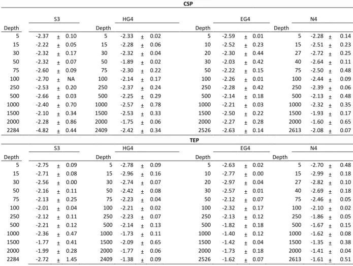
Table S7 Size frequency distribution coefficients δ for both gel particle types, at all stations and all depths. Numbers represent means of the two replicate samples, standard deviation is indicated after ±. NA means that standard deviation was not calculable due to one missing replicate. Depths for each station are shown in meters.
CSP
S3
HG4 EG4 N4
Depth Depth Depth Depth
5 -2.37 ± 0.10 5 -2.33 ± 0.02 5 -2.59 ± 0.01 5 -2.28 ± 0.14
15 -2.22 ± 0.05 15 -2.28 ± 0.06 10 -2.52 ± 0.23 15 -2.51 ± 0.23
30 -2.32 ± 0.17 30 -2.32 ± 0.04 20 -2.30 ± 0.44 27 -2.72 ± 0.25
50 -2.32 ± 0.07 50 -1.89 ± 0.02 30 -2.03 ± 0.42 40 -2.64 ± 0.11
75 -2.60 ± 0.09 75 -2.30 ± 0.22 50 -2.22 ± 0.15 75 -2.50 ± 0.48
100 -2.70 ± NA 100 -2.14 ± 0.17 100 -2.26 ± 0.01 100 -2.44 ± 0.09
250 -2.53 ± 0.20 250 -2.37 ± 0.24 250 -2.28 ± 0.42 250 -2.39 ± 0.06
500 -2.66 ± 0.03 500 -2.25 ± 0.29 500 -2.14 ± 0.18 500 -2.13 ± 0.48
1000 -2.40 ± 0.70 1000 -2.57 ± 0.78 1000 -2.21 ± 0.03 1000 -2.32 ± 0.35
1500 -2.10 ± 0.34 1500 -2.53 ± 0.33 1500 -2.50 ± 0.22 1500 -1.93 ± 0.17
2000 -2.28 ± 0.86 2000 -1.75 ± 0.06 2000 -2.27 ± 0.28 2000 -1.60 ± 0.65
2284 -4.82 ± 0.44 2409 -2.42 ± 0.34 2526 -2.63 ± 0.14 2613 -2.08 ± 0.07
TEP
S3 HG4 EG4 N4
Depth Depth Depth Depth
5 -2.75 ± 0.09 5 -2.78 ± 0.09 5 -2.63 ± 0.02 5 -2.70 ± 0.48
15 -2.71 ± 0.08 15 -2.96 ± 0.16 10 -2.77 ± 0.00 15 -2.99 ± 0.18
30 -2.56 ± 0.00 30 -2.74 ± 0.07 20 -2.97 ± 0.04 27 -2.82 ± 0.10
50 -2.16 ± 0.11 50 -2.42 ± 0.08 30 -2.57 ± 0.01 40 -2.69 ± 0.18
75 -2.13 ± 0.25 75 -2.23 ± 0.04 50 -2.12 ± 0.07 75 -2.46 ± 0.05
100 -2.01 ± 0.04 100 -2.21 ± 0.02 100 -2.32 ± 0.17 100 -2.10 ± 0.02
250 -2.12 ± 0.11 250 -2.23 ± 0.07 250 -2.13 ± 0.12 250 -1.86 ± 0.05
500 -2.21 ± 0.12 500 -2.14 ± 0.13 500 -1.82 ± 0.18 500 -1.67 ± 0.15
1000 -2.36 ± 0.47 1000 -1.73 ± 0.11 1000 -1.40 ± 0.12 1000 -1.62 ± 0.08
1500 -1.77 ± 0.41 1500 -2.09 ± 0.65 1500 -1.42 ± 0.04 1500 -1.35 ± 0.38
2000 -1.99 ± 0.28 2000 -1.77 ± 0.06 2000 -1.73 ± 0.18 2000 -1.41 ± 0.04
2284 -2.72 ± 1.45 2409 -1.38 ± 0.09 2526 -1.62 ± 0.07 2613 -1.61 ± 0.51
S8 Multi-focus stack (created from several pictures taken while focussing through the aggregate) of two aggregates derived from the Marine Snow Catcher, stained with Alcian Blue (left) or Coomassie Brilliant Blue G (right). The scale bar, which is only valid for each enlarged section, represents 10µm. The total aggregate length of the left aggregate was measured to be 410µm, the total aggregate length of the right aggregate was measured to be 520µm. Micrographs were taken by bright-field microscopy.
Table S9 Size (of particle) - frequency (of bacteria) distribution coefficients a and b for both gel particle types (TEP and CSP) over depth at all four stations (S3, HG4, EG4, N4).
Numbers in brackets after 'TEP' or 'CSP' indicate water depths in meters. Depths indicated with '~' represent median between the four stations (as sampling depths in the euphotic zone were slightly adjusted at each station to sample the chlorophyll maximum and its gradient).
'>2000m' refers to depths below 2000m.
S 3 HG 4 EG 4 N 4
Particle type a b a b a b a b
TEP (5m) x 0.372 x 1.167 x 0.880 x 0.611 x 0.680 x 0.908 x 1.929 x 0.236 TEP (~15m) x 1.345 x 0.401 x 1.236 x 0.354 x 0.724 x 0.720 x 0.407 x 1.046 TEP (~30m) x 1.039 x 0.625 x 0.784 x 0.605 x 1.655 x 0.304 x 0.350 x 1.025 TEP (~45m) x 0.838 x 0.821 x 0.557 x 0.846 x 0.801 x 0.740 x 0.567 x 0.741 TEP (~75m) x 0.907 x 0.793 x 1.485 x 0.420 x 0.871 x 0.756 x 1.471 x 0.349 TEP (100m) x 1.172 x 0.686 x 0.978 x 0.577 x 2.090 x 0.154 x 0.294 x 1.013 TEP (250m) x 0.664 x 0.966 x 0.681 x 0.581 x 1.545 x 0.352 x 1.695 x 0.248 TEP (500m) x 0.786 x 0.757 x 2.635 x -0.066 x 0.791 x 0.798 x 0.887 x 0.614 TEP (1000m) x 2.479 x 0.304 x 0.696 x 0.783 x 0.803 x 0.586 x 1.908 x 0.107 TEP (1500m) x 1.921 x 0.110 x 1.168 x 0.356 x 0.875 x 0.632 x 0.837 x 0.616 TEP (2000m) x 0.137 x 1.311 x 0.000 x 4.924 x 0.336 x 0.951 x 1.380 x 0.338 TEP (>2000m) x 1.136 x 0.257 x 1.140 x 0.407 x 1.191 x 0.331 x 0.713 x 0.608 CSP (5m) x 0.822 x 0.754 x 0.266 x 1.068 x 1.076 x 0.493 x 1.896 x 0.233 CSP (~15m) x 0.908 x 0.808 x 0.341 x 0.966 x 0.888 x 0.474 x 0.648 x 0.659 CSP (~30m) x 1.291 x 0.452 x 0.393 x 1.084 x 0.133 x 1.397 x 5.687 x -0.141 CSP (~45m) x 0.348 x 0.999 x 0.093 x 1.372 x 0.919 x 0.499 x 1.810 x 0.245 CSP (~75m) x 2.829 x -0.036 x 1.063 x 0.289 x 1.174 x 0.413 x 0.155 x 1.231 CSP (100m) x 1.542 x 0.299 x 1.563 x 0.201 x 1.448 x 0.375 x 0.810 x 0.541 CSP (250m) x 0.962 x 0.504 x 2.115 x 0.180 x 1.261 x 0.405 x 4.630 x -0.158 CSP (500m) x 1.810 x 0.203 x 2.000 x 0.000 x 1.000 x 0.377 x 0.097 x 1.269 CSP (1000m) x 2.999 x -0.005 x 0.649 x 0.620 x 1.901 x 0.181 x 2.000 x 0.000 CSP (1500m) x 2.705 x 0.040 x 4.327 x -0.221 x 2.740 x -0.066 x 1.451 x 0.217 CSP (2000m) x 0.907 x 0.645 x 0.005 x 2.490 x 1.854 x 0.135 x 2.000 x 0.000 CSP (>2000m) x 7.545 x -0.423 x 1.532 x 0.214 x 12.340 x -0.477 x 1.249 x 0.288