der Bayerischen Akademie der Wissenschaften
Reihe C Dissertationen Heft Nr. 771
Janja Avbelj
Fusion of Hyperspectral Images and Digital Surface Models for Urban Object Extraction
München 2016
Verlag der Bayerischen Akademie der Wissenschaften in Kommission beim Verlag C.H.Beck
ISSN 0065-5325 ISBN 978-3-7696-5183-6
Diese Arbeit ist gleichzeitig veröffentlicht in:
DLR-Forschungsberichte; ISSN 1434-8454; Nr. ISRN DLR-FB--2016-07; Köln 2016
der Bayerischen Akademie der Wissenschaften
Reihe C Dissertationen Heft Nr. 771
Fusion of Hyperspectral Images and Digital Surface Models for Urban Object Extraction
Vollständiger Abdruck
der von der Ingenieurfakultät Bau Geo Umwelt der Technischen Universität München zur Erlangung des akademischen Grades eines
Doktor-Ingenieurs (Dr.-Ing.) genehmigten Dissertation
von
Janja Avbelj
München 2016
Verlag der Bayerischen Akademie der Wissenschaften in Kommission bei der C.H.Beck'schen Verlagsbuchhandlung München
ISSN 0065-5325 ISBN 978-3-7696-5183-6
Diese Arbeit ist gleichzeitig veröffentlicht in:
DLR-Forschungsberichte; ISSN 1434-8454; Nr. ISRN DLR-FB--2016-07; Köln 2016
Deutsche Geodätische Kommission
Alfons-Goppel-Straße 11 ! D – 80539 München
Telefon +49 – 89 – 230311113 ! Telefax +49 – 89 – 23031-1283 /-1100 e-mail hornik@dgk.badw.de ! http://www.dgk.badw.de
Prüfungskommission
Vorsitzender: Univ.-Prof. Dr.-Ing. habil. Xiaoxiang Zhu
Prüfer der Dissertation: 1. Univ.-Prof. Dr.-Ing. habil. Richard H. G. Bamler
2. Hon.-Prof. Dr.-Ing. Peter Reinartz, Universität Osnabrück 3. 3. Prof. Dr.-Ing. Markus Gerke, University of Twente, Niederlande
Die Dissertation wurde am 16.09.2015 bei der Technischen Universität München eingereicht und durch die Ingenieurfakultät Bau Geo Umwelt am 20.11.2015 angenommen.
.
Diese Dissertation ist auf dem Server der Deutschen Geodätischen Kommission unter <http://dgk.badw.de/>
sowie auf dem Servern der Technischen Universität München / des Deutschen Zentrums für Luft- und Raumfahrt (DLR) unter
<https://mediatum.ub.tum.de./node?id=1275953> / <http://elib.dlr.de/100607/> elektronisch publiziert
Die Dissertation ist erstveröffentlicht als Forschungsbericht des Deutschen Zentrums für Luft- und Raumfahrt unter: Avbelj, Janja:
Fusion of Hyperspectral Images and Digital Surface Models for Urban Object Extraction, DLR-Forschungsbericht 2016, Köln, ISRN DLR-FB--2016-07 (zugleich Dissertation Technische Universität München 2015)
und parallel online freigeschaltet unter <http://elib.dlr.de>
© 2016 Deutsche Geodätische Kommission, München
Alle Rechte vorbehalten. Ohne Genehmigung der Herausgeber ist es auch nicht gestattet,
die Veröffentlichung oder Teile daraus auf photomechanischem Wege (Photokopie, Mikrokopie) zu vervielfältigen
ISSN 0065-5325 ISBN 978-3-7696-5183-6
Summary
Buildings are prominent objects of the constantly changing urban environment. Accurate and up to date Building Polygons (BP) are needed for a variety of applications, e.g. 3D city visualisation, micro climate forecast, and real estate databases. The increasing number of earth observation remote sensing images enables the development of methods for building extraction. For instance, Hyperspectral Images (HSI) are a source of information about the material of the objects in the scene, whereas the Digital Surface Models (DSM) carry information about height of the surface and of objects. Thus, complementary information from multi-modal images, such as HSI and DSM, is needed to provide better understanding of the observed objects. A variation in material and height is represented by an edge in HSI and DSM, respectively. Edges in an image carry large portions of information about the geometry of the objects, because they delineate the boundaries between them. Object extraction and delineation is more reliable if information content from HSI, DSM, and edge information is jointly accounted for. The focus in this thesis is on method development for BP extraction using complementary information from HSI and DSM by accounting for edge information. Furthermore, a new quality measure, which accounts for shape dierences and geometric accuracy between extracted and reference polygons, is proposed.
Object and edge detection from an image is meaningful only for some range of scales. Edge detection in scale space is motivated by showing that in the same image dierent edges appear at dierent scales.
Instead of deterministic edge detection, edge probabilities are computed in a linear scale space. Bayesian fusion of edge probabilities is proposed, which employs a Gaussian mixture model. The scale, at which an edge probability is computed, is dened by a condence probability. The impact of selecting mixing coecients in the Gaussian mixture model according to a prior knowledge or by a fully automatic data-driven approach is investigated. Main limitations of joining the edge probabilities from dierent datasets are the coregistration between the datasets and the inaccuracies in the datasets.
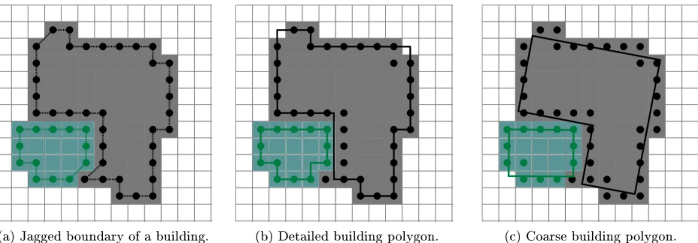
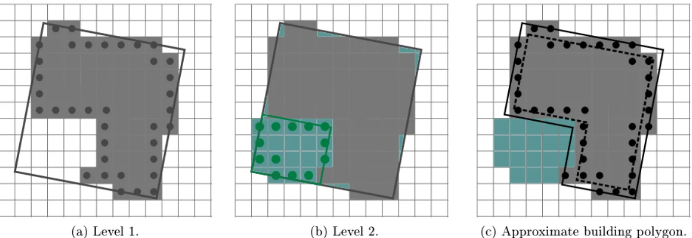
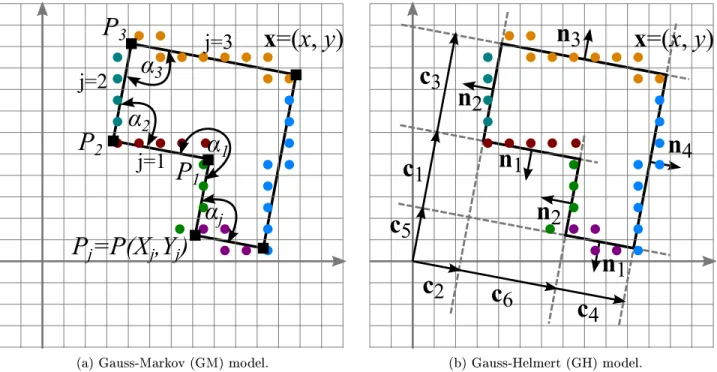
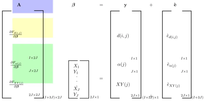
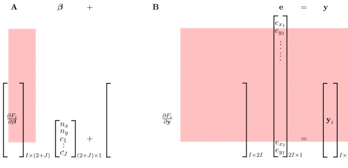
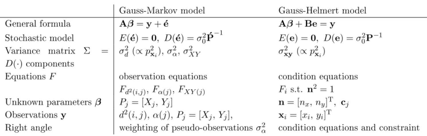
The rectilinear BP are adjusted by means of weighted least squares, where the weights are dened on the basis of joint edge probabilities. Two mathematical models for rectilinear BP are proposed, one with a strict rectilinearity constraint and the second one, which introduces a relaxed rectilinearity constraint through weighting. The experiments on synthetic images show that the model with strict constraint gives better results, if the BP under consideration are all rectilinear. Otherwise, the relaxed rectilinearity constraint through weighting balances better between the rectilinearity assumption and tness to the data. The approximate BP are created by a Minimum Bounding Rectangle (MBR) method. A main contribution of the proposed iterative MBR method is the automatic selection of a level of complexity of MBR through analysis of a cost function.
A metric for comparison of polygons and line segments, named PoLiS metric, is dened. It compares polygons with dierent number of vertices, is insensitive to the number of vertices on polygon's edges, is monotonic, and has a nearly linear response to small changes in translation, rotation, and scale. Its characteristics are discussed and compared to the commonly used measures for BP evaluation. In all experiments the BP are evaluated by computing the newly proposed PoLiS metric and quality rate.
The feasibility of joining all the proposed methods in one workow is shown through the experiment,
which is carried out on 17 HSI-DSM dataset pairs with four dierent ground sampling distances. The
main nding of the experiment is that joining the information from multi-modal images, i.e. HSI and
DSM, results in better quality of the adjusted BP. For instance, even for datasets with 4 m ground
sampling distance, the completeness, correctness and quality rate values of extracted BP are better
than 0.83, 0.68, and 0.60. Inaccuracies of the images, such as holes in DSM or imperfect DSM for HSI
orthorectication, are inuencing the accuracy and localisation of edge probabilities and consequently
also the accuracy of adjusted BP.
Zusammenfassung
Gebäude sind in einem sich stetig verändernden städtischem Raum von besonderem Interesse. Genaue und immer aktuelle Gebäudeumrisse werden in einer Vielzahl von Anwendungen benötigt, wie z.B. für 3D Städtemodelle, Mikroklima-Vorhersagen oder auch Grundstücksdatenbanken. Die Entwicklung von Methoden zur Gebäudeextraktion aus Erdbeobachtungsdaten, insbesondere aus Bilddaten, wird durch deren steigende Verfügbarkeit stetig vorangetrieben. So geben Hyperspektralbilddaten (HSI) zum Bei- spiel Aufschluss über das Gebäudematerial in einem Gebiet, wohingegen Oberächenmodelle (DSM) vom gleichen Gebiet Informationen über den Geländeverlauf und die Höhe der Gebäude enthalten. Um die Gebäudeeigenschaften in einem Gebiet genauer auswerten zu können, sind sich ergänzende Informa- tionen von multimodalen Bilddaten, wie HSI und DSM, nötig. Räumliche Änderungen von Materialien erzeugen in einem HSI eine Kante wogegen eine Kante in einem DSM durch Höhenunterschiede erzeugt wird. Kanten enthalten also Informationen über Gebäudeeigenschaften, weil sie Grenzen zwischen Ob- jekten darstellen. Die Extraktion von Gebäuden und die Bestimmung ihrer Umrisse sind zuverlässiger, wenn der Informationsgehalt aus HSI, DSM und Kanteninformationen gemeinsam in Betracht gezogen wird. Der Schwerpunkt dieser Doktorarbeit liegt in der Entwicklung von Methoden zur Extraktion von Gebäudeumrissen aus sich ergänzenden Informationen von HSI und DSM durch Betrachtung der Kanteninformationen.
Gebäude- und Kantendetektion in einem Bild sind nur in bestimmten Skalen aussagekräftig. Kan- tendetektion im Skalenraum ist dadurch motiviert, dass im selben Bild unterschiedliche Kanten in unterschiedlichen Skalenräumen existieren. Anstelle von deterministischer Kantendetektion werden Kantenwahrscheinlichkeiten im linearen Skalenraum berechnet und unter Verwendung eines gauÿschen Mischungsverteilungsmodells eine bayesianische Fusion von Kantenwahrscheinlichkeiten durchgeführt.
Die Skala in der eine Kantenwahrscheinlichkeit berechnet wird, ist durch die Kondenzwahrschein- lichkeit deniert. Der Einuss einer a priori gesteuerten und einer automatisch datengesteuerten Be- stimmung der Mischungsgewichte im gauÿschen Mischverteilungsmodell wird untersucht. Die gröÿte Limitierung bei der Kombination von Kantenwahrscheinlichkeiten aus verschiedenen Datensätzen ist die Ungenauigkeit der Koregistrierung zwischen den Datensätzen und die Ungenauigkeit der einzelnen Datensätze.
Rechtwinklige Gebäudepolygone werden durch die Methode der kleinsten Quadrate berechnet, wobei die Gewichtung in der Ausgleichung auf den kombinierten Kantenwahrscheinlichkeiten basiert. Zwei mathematische Modelle zur Berechnung von rechtwinkligen Gebäudepolygonen werden vorgestellt. Die erste Methode beruht auf einer strengen Rechtwinkligkeit und in der zweiten Methode wird die Be- dingung der Rechtwinkligkeit durch Gewichtungsfaktoren relaxiert. Untersuchungen mit synthetischen Bilddaten zeigen, dass die Methode mit streng rechtwinkligker Beschränkung bessere Ergebnisse lie- fert, wenn die untersuchten Gebäudestrukturen tatsächlich rechtwinklig sind. Andererseits liefert die Methode basierend auf Gewichtsfaktoren ein ausgewogeneres Ergebnis bezüglich Rechtwinkligkeit und Passgenauigkeit der Daten. Die approximierten Gebäudepolygone werden mit der Methode der mi- nimal umgebenden Rechtecke (MBR) erstellt. Ein Hauptbeitrag zur iterativen MBR-Methode ist die automatische Auswahl einer Komplexitätsebene der MBR durch die Analyse einer Kostenfunktion.
Es wird eine Metrik zum Vergleich von Polygonen und Liniensegmenten, die PoLiS-Metrik, vorgestellt.
Die PoLiS-Metrik erlaubt Vergleiche von Polygonen mit unterschiedlicher Anzahl von Kanten, ist
unempndlich gegenüber der Eckenanzahl einer Polygonseite, ist monoton und zeigt ein fast lineares
Verhalten für kleine Veränderungen in Translation, Rotation und Maÿstab. Die Charakteristiken der
PoLiS-Metrik werden diskutiert und mit auf diesem Forschungsgebiet anerkannten Qualitätsmaÿen für
Gebäudestrukturen verglichen. Die Gebäudestrukturen werden in allen Versuchen durch die vorgestellte
PoLiS-Metrik und eine bekannte Qualitätsrate evaluiert.
Die Möglichkeit alle vorgestellten Methoden in einen Gesamtprozess einzubinden, wird durch einen Versuch an 17 HSI-DSM Datensatzpaaren mit vier verschiedenen Bodenauösungen gezeigt. Eine we- sentliche Erkenntnis aus diesem Versuch ist, dass die Kombination von Informationen aus multimodalen Bilddaten, z.B. HSI und DSM, ein qualitativ besseres Ergebnis der ausgeglichenen Gebäudepolygone liefert. Zum Beispiel sind für Datensätze mit 4 m Bodenauösung die Richtig-Positiv-Rate (Vollstän- digkeit, completeness), der positive Vorhersagewert (correctness) und die Qualitätsrate (quality rate) der extrahierten Gebäudepolygone besser als 0.83, 0.68 und 0.60. Ungenauigkeiten der Bilder, wie z.B.
Lücken im DSM oder ein ungenaues DSM für die HSI Orthorektizierung, beeinussen die Genau-
igkeit und Lokalisierung von Kantenwahrscheinlichkeiten und infolgedessen auch die Genauigkeit der
ausgeglichenen Gebäudepolygone.
Contents
1 Introduction 11
1.1 Scientic Relevance of the Topic . . . . 11
1.2 Objectives and Focus of the Thesis . . . . 12
1.3 Outline . . . . 13
2 Theoretical Background 15 2.1 Hyperspectral Imaging . . . . 15
2.1.1 Terminology and Basic Principles of HSI . . . . 15
2.1.2 Distortions in HSI and Their Characteristics . . . . 17
2.2 Digital Elevation Models . . . . 21
2.2.1 Terminology . . . . 21
2.2.2 DEM Generation and Their Characteristics . . . . 21
2.3 Image Fusion in Urban Areas . . . . 24
2.3.1 Availability of the Multi-View and Hyperspectral Images . . . . 25
2.3.2 Potential and Challenges of the HSI and DSM Fusion . . . . 25
3 Advances in HSI and DSM Fusion for Building Extraction 29 3.1 Building Extraction from Remote Sensing Data . . . . 29
3.1.1 General Workow of Geometrical Building Extraction . . . . 30
3.1.2 Least Squares Adjustment of Rectilinear Building Outlines . . . . 32
3.2 Remote Sensing and Scale Space . . . . 33
3.3 Evaluation of Building Outline Extraction . . . . 35
3.3.1 Wild West in Evaluation Techniques for Extracted Building Polygons . . . . 35
3.3.2 Overview of Indices . . . . 36
3.3.3 What is Ground Truth? . . . . 37
3.4 Summary of Research Voids . . . . 38
4 Fusion of HSI and DSM 39 4.1 Edge in an Image . . . . 39
4.1.1 Edge Detection and Edge Probability in an Image . . . . 42
4.1.2 Scale Space Representation . . . . 45
4.1.3 Implementation of the Discrete Linear Scale Space and Scale Space Derivatives 46
4.2 Bayesian Fusion of HSI and DSM Based on Edges . . . . 48
4.2.1 Abundance and Probability of an Edge . . . . 48
4.2.2 DSM Derived Probability of an Edge . . . . 48
4.2.3 Gaussian Mixture Model . . . . 49
4.3 Information Content Relation of HSI and DSM . . . . 49
4.3.1 Weighting by Prior Knowledge . . . . 50
4.3.2 Weighting by Data-Based Condence Level . . . . 50
5 Building Outline Extraction and Adjustment 51 5.1 Approximate Building Outline Determination . . . . 51
5.1.1 Building Region Extraction . . . . 51
5.1.2 Building Polygon Creation and Selection . . . . 53
5.2 Joined use of HSI and DSM for Building Polygon Estimation . . . . 55
5.2.1 Mathematical Model for Rectilinear Polygon . . . . 56
5.2.2 Weights in the Adjustment . . . . 60
5.3 A New Metric for Evaluation of Polygons and Line Segments (PoLiS) . . . . 62
5.3.1 Measures for Quantication of Similarity . . . . 63
5.3.2 Denition of the PoLiS Metric . . . . 70
5.3.3 Characteristics of the PoLiS Metric . . . . 71
6 Case Studies 79 6.1 Data Description and Preprocessing . . . . 79
6.1.1 HSI Sensors and Images . . . . 79
6.1.2 DSM from Stereo Images and LiDAR Point Clouds . . . . 82
6.1.3 Implementation and Setting of Parameters for Proposed Methods . . . . 82
6.2 Experiments on Scale Space for Edge Detection . . . . 83
6.2.1 Test Dataset . . . . 83
6.2.2 Parameter Settings . . . . 84
6.2.3 Results and Discussion . . . . 84
6.2.4 Summary of Experiments on Scale Space for Edge Detection . . . . 89
6.3 Experiment on Building Polygon Selection and Adjustment . . . . 90
6.3.1 Test Dataset . . . . 90
6.3.2 Parameter Settings . . . . 92
6.3.3 Results and Discussion of the Model Selection Experiment . . . . 93
6.3.4 Results and Discussion of the Adjustment . . . . 96
6.3.5 Summary of Experiment on BP Selection and Adjustment . . . 101
6.4 Experiments on RS Images . . . 102
6.4.1 Test Dataset . . . 102
6.4.2 Parameter Settings and Preprocessing . . . 104
6.4.3 Results and Discussion of the Experiment on the Small Area . . . 105
6.4.4 Results and Discussion of the Experiment on the Large Area . . . 114
6.4.5 Summary of Experiments on RS Images . . . 121
7 Conclusions and Outlook 123 7.1 Conclusions . . . 123
7.2 Outlook . . . 124
Acronyms 127
List of Figures 129
List of Tables 132
Bibliography 133
Acknowledgements 141
1 Introduction
A picture is worth a thousand words! This proverb becomes a new dimension when a picture is a Hyperspectral Image (HSI) with dozens or even hundreds of spectral bands. How many words is the HSI worth? The HSI is a source of information about geometry and materials of objects in the image. If besides the HSI also a Digital Surface Model (DSM) is available, which is a source of information about geometry and heights of objects, the joined information value from both datasets is further increased. Thus, the HSI and DSM carry complementary information about the covered area.
Moreover, a variation in material and height is represented by edges in HSI and DSM, respectively.
More reliable discrimination and delineation of the objects is possible by extracting the knowledge about the edges from these images. The information value from HSI, DSM, and the edge information together are worth more than thousands of words.
The topic of this thesis is the usage of the hyperspectral images and digital surface models for urban object extraction. In order to detect building polygons from HSI and DSM, a method for rectilinear building polygon extraction is proposed, which accounts for edge probabilities from both datasets.
A new quality measure for evaluation of the extracted building polygons, called Polygons and Line Segments (PoLiS) metric, is dened and compared to the already community accepted measures.
1.1 Scientic Relevance of the Topic
The variety of applications, such as 3D city visualisation, micro climate forecast and monitoring, real estate databases, require up to date building polygons or models as an input (Brédif et al., 2013;
Rottensteiner et al., 2014). The City Geography Markup Language (CityGML), an international standard on city models describes representation, storage, and exchange of the 3D city models (Gröger and Plümer, 2012). The European Union also issued specications about buildings and their properties within the Infrastructure for Spatial Information in Europe (INSPIRE) framework (INSPIRE TWG BU, 2013). The 3D geometry at dierent Level of Detail (LOD), semantics, and material attributes of building façades and roofs is specied in both, the CityGML standard and INSPIRE framework (Avbelj et al., 2015a; Gröger and Plümer, 2012; INSPIRE TWG BU, 2013).
Air- or space-borne Remote Sensing (RS) enable periodic acquisitions of images of larger areas. The increasing number and availability of the Earth Observation (EO) RS images enables the development of methods for building extraction, which combine several datasets (Brenner, 2005; Gamba, 2014;
Hu et al., 2003). The complementary information from multi-modal RS imagery can be exploited for building extraction. Typically, one of the datasets exhibits heights of the objects, e.g. DSM and Light Detection and Ranging or Light Radar (LiDAR) point cloud, and the other one the spectral characteristics of the objects in the scene, e.g. HSI and Multispectral (MS). HSI provide, in contrast to MS images, material information about building façades and roofs, as specied in CityGML and INSPIRE framework.
The geometry of the objects in the scene can be extracted from RS images. The accuracy, with which the geometry of an object can be extracted, depends on the characteristics of an image. Spatial resolution, one of the characteristics of the RS images, limits the smallest extractable detail of an object. MS images provide higher spatial (and lower spectral) resolution in comparison to the HSI.
However, some air-borne HSI sensors, e.g. HyMAP, HySpex, and AVIRIS, acquire images with not
only high spectral, but also better spatial resolution. Better spatial resolution enables extraction of
smaller objects common for urban areas. Also the future EO HSI missions, such as EnMAP, DESIS,
HyspIRI, motivate further developments of the methods for automatic urban object extraction from
HSI. The building extraction on the basis of material properties in HSI is a widely addressed research topic (e.g. Roessner et al., 2001; Segl et al., 2003a). Only few researchers addressed the problem of extracting polygons, and not pixel regions, of the objects from HSI (Avbelj et al., 2013a, 2015a; Brook et al., 2010; Huertas et al., 1999).
Inaccuracies of acquisition techniques of RS sensors and processing methods inuence the values in the images (Eismann, 2012; Richards and Jia, 2006). These inaccuracies are usually corrected for.
Nevertheless, not only random, but also some uncorrected systematic errors may remain in the images and have to be dealt with when extracting objects and their edges. These uncorrected systematic errors are a limiting factor to the accuracy of extracted objects. Thus, the methods for extracting building polygons from HSI must be robust against these uncorrected errors.
Edges in an image carry large portions of information about the geometry of objects, because they delineate the boundaries between them. If the boundaries of the same object can be extracted from multi-modal RS images with dierent characteristics, such as DSM and HSI, then they can be used as the basis for image fusion. The same object, mapped to an image of coarser scale, might not be extractable. Thus, object and edge detection from an image is meaningful only for some range of scales (Lindeberg, 1998). Moreover, dierent edges in the image can appear at dierent scales (Koenderink, 1984; Lindeberg, 1994; Witkin, 1984). The edge detection in RS images at dierent scales has a potential to provide better results than single scale edge detector algorithms (Field and Brady, 1997;
Lindeberg, 1994, 1998; Lowe, 1999; Marimont and Rubner, 1998; Perona and Malik, 1990), e.g. Canny (Canny, 1986). The analysis of the necessity of scale space edge detection from RS images has not been analysed so far. The main goal of this thesis is to extract building polygons by accounting for edge information from HSI and DSM to increase their quality (Avbelj et al., 2013b). This is achieved by adjustment process of the extracted building polygons, which accounts for fused edge probability information.
The extracted polygons have to be evaluated with regard to ground truth. A shortage of standard evaluation techniques for extracted polygons has been addressed by several authors (e.g. Awrangjeb et al., 2010; Ragia and Winter, 2000; Rottensteiner et al., 2014, 2007; Zeng et al., 2013; Zhan et al., 2005). A further goal is therefore to propose a single evaluation measure, which accounts for shape and geometric accuracies of the extracted polygon, but is at the same time insensitive to the dierence in LOD between extracted and ground truth polygons (Avbelj et al., 2015b).
1.2 Objectives and Focus of the Thesis
Urban areas are characterised by a large number of objects on a relatively small area. The diversity of objects in urban environments can be described by the variation in size, shape, height, and material.
These characteristics of urban objects are well captured by HSI and DSM images. Both datasets should be jointly considered to gain a higher information value. Edge information is used to dene shape and location of the objects. The focus of this thesis is method development for building polygon extraction from HSI and DSM by accounting for edge information. The quality of extracted building shapes and the improvement of the geometric accuracy, when incorporating the edge information from HSI and DSM, have to be quantitatively evaluated. Thus, a single quality measure is needed, which accounts for shape dierences and geometric accuracy between extracted and ground truth polygons. Therefore, three major and one minor objectives are to be fullled:
Objective 1: Fusion of HSI and DSM based on edge information.
The information content of the image edges shall be extracted by computing edge probabilities in the
two modalities. The fact that edges in a single image can appear at dierent scales has to be accounted
for by edge probability computation in scale space. Necessity and potential of edge probability com- putation in scale space from RS images has to be analysed. Edge probabilities extracted from dierent multi-modal images have to be fused. The fusion according to prior knowledge or automatically by a fully data-driven approach has to be investigated.
Objective 2: Mathematical description and adjustment of rectilinear building polygons.
The rectilinear building polygons have to be described by a mathematical model in order to be es- timated by means of Least Squares (LS). The comparison of the strict and relaxed rectilinearity constraint in the model has to be investigated. The model has to allow for incorporation of edge information. Input parameters to the adjustment are approximate building polygons, which have to well represent the building outline in the image, i.e. the approximate building polygon has to balance between the details and generalisation of the building outline.
Objective 3: Denition of a new metric for evaluation of extracted building polygons.
A new metric for comparison of building polygons is needed, which accounts for positional accuracy and shape dierences between an extracted and a reference polygon. The metric shall have the following characteristics. It compares polygons with dierent number of vertices, is insensitive to the number of vertices on polygons' edges, is monotonic, and has a linear response to small changes in translation, rotation, and scale. It is a metric in a mathematical sense. The characteristics of the new metric shall be discussed and compared to the community accepted measures, e.g. matched rates and Root Mean Square Error (RMSE).
Minor objective: Joining the proposed methods (Objectives 1, 2, 3) in one workow.
Building polygon extraction and adjustment from HSI and DSM with various spatial resolutions shall be carried out to demonstrate the applicability of the proposed methods. The fused edge information from both datasets has to be included in the adjustment. The preprocessing steps of the HSI and the DSM such as DSM normalisation, and material map generation using unmixing of the HSI has to be carried out. The adjusted building polygons have to be evaluated by computing the newly proposed metric and commonly used evaluation measures.
1.3 Outline
The thesis is structured as follows. In this Chapter 1, the introduction is given, which includes scientic relevance of the topic and objectives of this thesis. Shortly, basics and characteristics of the HSI and DSM, followed by the overview of fusion of these two datasets for urban areas is given in Chapter 2.
The state of the art of building extraction and evaluation and the usage of scale space in RS images
are described, and research voids are identied in Chapter 3. The following two Chapters describe
methodological contributions. The edge in an image and edge probability computation in scale space
are introduced and the method for Bayesian fusion of edge probabilities is proposed in Chapter 4. The
method for building polygon extraction together with two adjustment models and the PoLiS metric
are proposed in Chapter 5. The experiments using the methods proposed in the previous two Chapters
are carried out and discussed in Chapter 6. First, the necessity of the edge probability detection
in scale space is shown. Second, the proposed method for building polygon extraction is applied on
synthetic images and the adjustment models are compared. Then, all proposed methods are joined in
one workow and applied on real HSIDSM dataset pairs. The results, ndings, and outlook on future
works are discussed in the nal Chapter 7.
2 Theoretical Background
The basic principles and characteristics of the two types of RS data, relevant for this thesis, HSI (Sec- tion 2.1) and DSM (Section 2.2), are introduced in this Chapter. Special focus is put on the inaccuracies of acquisition techniques and processing methods to the values in the images and DSM. Usually these inaccuracies are corrected for, nevertheless next to the random errors, some systematic errors can re- main uncorrected. Therefore, image processing methods must be robust towards these shortcomings.
Finally, an overview of image fusion of HSI and DSM in urban areas is given (Section 2.3).
2.1 Hyperspectral Imaging
Hyperspectral imaging (also called imaging spectroscopy or hyperspectral RS) is measuring electromag- netic radiation in tens or hundreds of mostly adjacent narrow spectral bands with increased spectral resolution in contrast to MS sensors with only few spectral bands (e.g.
≤12) of larger bandwidth andgaps between bands (Keshava, 2003; van der Meer, 2001). The abbreviation HSI is used for hyperspec- tral imaging and hyperspectral image. HSI sensors measure electromagnetic radiation in the optical spectral region (about 0.4-14 µ m). HSI used in this thesis are a result of a measured reected sun radiation in Visible and Near (VNIR) (about 0.4-1.1 µ m) and/or Short Wavelength Infrared (SWIR) (about 1.1-2.5 µm) spectral regions (Figure 2.1b). Therefore, the described principles and characteris- tics of the HSI are restricted to the passive HSI sensors acquiring data in VNIR and SWIR spectral regions. They dier in some aspects from the passive Thermal Infrared (TIR) HSI sensors measuring emitted thermal radiation (Eismann, 2012).
2.1.1 Terminology and Basic Principles of HSI
HSI from RS platforms simultaneously capture material information as well as spatial information of the observed scene. The resulting image can be regarded as a Three-Dimensional (3D) dataset, named also hypercube (Figure 2.1a), and is composed of N grey scale images, where N is the number of spectral bands or channels of the HSI. The spectral signature of each spatial pixel carries information of the surface contained in it. It depends on the chemical composition of the material, vibrational and electronic resonances of molecules of the material, microscopic surface and volumetric properties (Eismann, 2012, p.6).
The term pixel is used to describe the smallest element of a digital image, which represents a resolution cell in object space. The optical sensors are usually designed in a way that the maximum spatial sampling distance is approximately the same as a resolution cell. Thus, in optical imaging community and in this thesis, a pixel in an optical RS image is considered to describe also the resolution.
Material Identication from HSI
Materials present in a scene and captured in a HSI can be determined by computing a similarity
between the image and reference spectra, using unmixing techniques, or classication techniques. A
prerequisite for material identication is a known set of reference spectra of the materials. The existing
spectral libraries (Baldridge et al., 2009; Clark et al., 2007) include laboratory measured spectra with
high spectral resolution. Before image spectra can be compared to the laboratory measured spectra, the
HSI must be atmospherically corrected to ground reectance values and laboratory spectra resampled
to the spectral resolution of the HSI. To evade the complex atmospheric correction (Subsection 2.1.2),
the reference spectra can be manually or automatically (Plaza et al., 2004) extracted from the HSI.
Wavelength λ[µm]
λ=0.4
λ=2.5
channels
Spectral
dimension
Spatial dimension
Spatialdimension
(a) Hypercube.
0.5 1 1.5 2 2.5
0 20 40 60
V IS N IR
V N IR SW IR
Wavelength [µm]
Reflectance[%]
Vegetation Water
Red Roof Tiles
(b) Spectral signatures and typical spectral regions of HSI.
Figure 2.1: A HSI HyMAP image (Figure 2.1a) and three spectral signatures collected from it (Figure 2.1b). Six channels of HSI are shown, i.e. blue, green, and red in Visible (VIS) (a colour of a boundary of each channel is with respect to the wavelength colour), and three in SWIR portion of spectrum (grey boundary) (Figure 2.1a). Figure 2.1b shows spectral signatures of vegetation (green), water (dark blue) and red roong tiles, which were collected from the HyMAP image.
Left-right pointing arrows are showing the approximate extent of VIS, Near Infrared (NIR), VNIR, and SWIR portions of the spectrum.
The similarity between two spectra can be computed by dierent measures (Cerra et al., 2012; Robila and Gershman, 2005), e.g. (normalised) Euclidean distance, Mahalanobis distance, or through data compression (Cerra et al., 2011). Some of them are designed especially for HSI, for instance Spec- tral Angle Distance (SAD), which is also named cosinus distance or spectral angle mapper (SAM) (Kruse et al., 1993),
1spectral information divergence (Chang, 2000), or spectral correlation mapper (De Carvalho and Meneses, 2000).
In HSI unmixing literature the term endmember is used to describe spectra of so called pure or elementary material. The term reference spectra is used here instead of the term endmember because of the following two reasons. First, the concept of pure material is misleading, because materials with the same chemical composition can have dierent spectral response due to e.g. surface structure or reection characteristics. Second, the denition of an endmember varies depending on the application (Bioucas-Dias et al., 2012; Ma et al., 2014) and the spatial resolution of the HSI.
Some of the pixels in HSI consist of more than just one material and are called mixed pixels. A Linear Mixing Model (LMM) assumes that any observed pixel
x ∈RN, n
= 1, . . . , Nin the HSI ( N is the number of bands of the HSI) is a linear combination of the M, m
= 1, . . . , M, reference spectra vectors
sm ∈RNweighted by their abundances
a∈RM(e.g. Keshava, 2003). The M column vectors
smare arranged to a matrix with reference spectra
S∈RN×M. LMM is physically well founded if the mixing scale is macroscopic and incident light interacts with just one material (Bioucas-Dias et al., 2012).
A non-linear mixing model should be considered, when e.g. light scattered by multiple materials in a scene has a prominent inuence on the measured spectra (Keshava and Mustard, 2002; Ma et al., 2014). Let a HSI be denoted as a matrix
X ∈ RN×P, with columns holding the P, p
= 1, . . . , Pspectral vectors
xp ∈RNof the P pixels, then the LMM is given by
X=SA+N
(1)
1A reader with computer vision background should not confuse abbreviation of the SAD as a distance measure with a sum of absolute intensity dierences used in stereo matching methods.
where
A∈RM×Pis the abundance matrix, and
N∈RN×Pis a matrix of noise and modelling errors.
Abundances of each material can be considered as a material map of this material. Every material map has the same size like the size of any channel of the HSI.
Hyperspectral unmixing is the process of decomposition of the mixed pixels into the fractions or abundances of the constitute reference spectra (Keshava and Mustard, 2002). Let us assume a) LMM, b) Gaussian noise, and c) known all reference spectra
S, N > M . A Non-Constrained Least Squares (NCLS) solution for the abundance matrix
Aminimises the cost function
||X−SA||2Aˆ = arg min
A ||X−SA||2
, (2)
where
|| · ||2is the Euclidean L
2norm. The abundances should be positive to be meaningful in a physical sense, thus the cost function in Equation (2) is for the so called Non-Negative Least Squares (NNLS) subject to abundance non-negativity constraint
am,n ≥0, m= 1, . . . , M, n= 1, . . . , N.
(3) Additionally to the non-negativity constraint, the cost function in Equation (2) can be also subject to abundance sum-to-one constraint for every column p
= 1, . . . , Pof the
AM
X
m=1
am= 1.
(4)
This minimisation problem is called Fully-Constrained Least Squares (FCLS). The sum-to-one con- straint also has a physical meaning, because the sum of the fractional abundances for every spectral vector
xshould be exactly one. However, if the assumption c) does not hold, and not all reference spectra in a scene are known, then the FCLS will cause overtting of the model. Moreover, if an over-complete reference spectra matrix ( N < M ) from e.g. spectral libraries is given, then the sparse unmixing methods using L
0or L
1minimisation can be applied (Iordache et al., 2010). An extensive overview about HSI unmixing approaches can be found in Bioucas-Dias et al. (2012).
Alternative to the physical foundation of the LMM is the geometric or signal processing interpretation, which assumes that the reference spectra lie on the extremities of the M
−1simplex (Keshava, 2003;
Ma et al., 2014). Several methods for automatic reference spectra extraction, also called blind source separation in the signal processing community, use this assumption.
2.1.2 Distortions in HSI and Their Characteristics
Acquired HSI must be corrected for geometric and radiometric distortions. The geometric distortions cause incorrect location of the acquired area in an image, whereas the radiometric distortions cause distorted spectra (brightness of the pixels) of the captured area. The corrections, registration, and especially coregistration of the images are important factors within an image fusion framework. In this Subsection the main inuences on the HSI are summarised.
Spectral Distortions Due to the Atmosphere
The objective of hyperspectral imaging is to quantify the composition of the observed objects, thus the measured signal must be calibrated to physical meaningful units. The following quantities are dened for optical RS images.
Digital number [ ] is a dimensionless quantity measured by a sensor, e.g. MS, HSI.
Top of atmosphere
Clouds Scattering
EO platforms Solar irradiation
Digital number [ ]
Surface reflectance [%]
Earth's surface
Adjacency effect
At-sensor radiance [W m-2 sr-1 nm-2]
Absorption
Cal.
Tables
Absorption Atmosphere
Absorption Reflection BRDF effect
Pixel Adjacent pixel
Sky irradiance component
Path radiance component Direct
radiation
Path radiance component
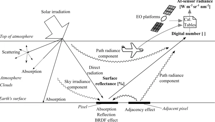
Figure 2.2: Atmospheric and other inuences on the radiance measured by a passive sensor. A measured radiance of an area on ground representing an image pixel is a result of dierent paths through the atmosphere (wavy lines). It depends also on the incident angle, surface properties, and sensor capabilities. Actual quantity measured by a sensor is a Digital Number (DN), which can be converted to at-sensor radiance by accounting for sensor-specic systematic inuences. The surface or ground reectance are additionally corrected for the atmospheric inuences. The gure is based on Richards and Jia (2006, p.28) and Eismann (2012, p.12).
At-sensor radiance has physically meaningful units, energy in unit time, unit area, unit solid angle, and unit wavelength [W m
−2sr
−1nm
−1]. It is computed from DN by accounting for sensor-specic systematic inuences. These calibration values are given by the producer of the sensors and by carrying out laboratory and in-ight calibration.
Top-of-atmosphere reectance [%] can be converted from at-sensor radiance values, e.g. for VNIR and SWIR spectral regions the radiance is divided by the incoming solar energy.
Ground or surface reectance [%] values are corrected also for the atmospheric inuences, e.g. re- ection, absorption, and scattering caused by clouds, particles, and absorption of some gases in the atmosphere (Figure 2.2).
The down-welling radiation as well as reected radiation are aected by the atmospheric inuences.
If the path through the atmosphere is longer, these inuences are larger. Scattering by aerosols and molecules in the atmosphere is the dominant component of the radiometric distortions (Richards and Jia, 2006, p. 2735). Figure 2.2 shows the main atmospheric inuences on the measured radiance values of a single pixel.
The reected signal is inuenced also by the properties of the surface. The Bidirectional Reectance
Distribution Function (BRDF) describes the reection of a non-Lambertian surface (opaque) under
varying solar and viewing geometry. Moreover, radiance values should also be corrected for adjacency
eects, i.e. reections and scattering from the neighbouring areas to the target. This eect has a larger
inuence in the areas with high-raising objects and rugged terrain, i.e. where the elevation dierences
on a small area are signicant. For instance, a wall of a building can cause multiple reections of
incoming solar radiation, which increases the proportion of adjacency eect in measured radiance.
Distortions Due to the Acquisition Technique: Whisk- and Push-Broom HSI Sen- sors
A typical acquisition technology for collecting HSI are push-broom line scanners, which use the move- ment of a platform to collect the along-track spatial dimension of the image. One row of an image, collected at the same time, is approximately perpendicular to the ight direction. Two examples of HSI push-broom sensors are the air-borne HySpex (Norsk Elektro Optikk AS, 1985) and the future space-borne EnMAP (EnMAP, 2015). Another acquisition technology are whisk-broom sensors, such as the air-borne HyMap sensor, which reect incoming light with rotating optics onto a single linear detector and collect the data across-track. This causes scan time distortion, because the data of one image line are collected from the S-shape area on the ground. The whisk-broom sensors have shorter dwell time causing lower Signal to Noise Ratio (SNR) in comparison to the push-broom sensors. Yet, the latter require extensive calibration, because each row of photo detectors of the Two-Dimensional (2D) array is eectively its own spectrometer. The limited dwell time and the moving scanning optics of the whisk-broom sensors are the main reason that the push-broom HSI sensors are preferred for space-borne missions. However, the opening angle of the optics or Field of View (FOV) is usually larger for the whisk-broom sensors, and therefore also (for the same altitude of a platform) the swath width. Another acquisition technology are frame sensors, which collect a spectral image in two spatial directions at the same time. Frame HSI sensors have lower SNR and are more commonly used on unmanned aerial platforms. Therefore, this acquisition technology is not further discussed.
For push-broom sensors, the incoming light passes through a slit and is diracted by a grating element or a prism into the wavelength components, which fall onto the 2D array of a (photo) detector, shortly referred to as 2D array. The 2D array has a spectral and a spatial dimension. The number of detectors in spatial dimension of the 2D array is the number of pixels of an image in across-track direction, and the number of detectors in the spectral dimension is equal to the number of spectral channels.
The optical properties of an HSI sensor cause that the HSI are distorted. Therefore, the spectral and geometric (spatial) characteristics of an optical sensor must be measured. The optical properties are connected to the detector and acquisition technology (Yokoya et al., 2010), i.e. linear detector for whisk- broom sensors and 2D detector array for push-broom sensors. Spectral characteristics of detectors are described by a Spectral Response Function (SRF). Let us assume that the SRF of every detector can be described by a Gaussian. Then, the SRF of every detector is given by a central wavelength, i.e. peak sensitivity of a detector, and the Full Width at Half Maximum (FWHM). The geometric properties of the detector are described by the Line Spread Function (LSF). The LSF are dierent for along- and across-track directions and are characterised by the centre angles and their FWHM (Baumgartner et al., 2012; Mouroulis et al., 2000).
The response of an imaging system to a point source is described by the Point Spread Function (PSF).
A simplied representation of the 2D PSF (in the zeroth order) is an ellipse. The semi-axes of the ellipse are here referred to as spatial and spectral semi-axis. Let a regular grid be assumed. If no distortions are present, the peaks of the PSF are aligned in spectral and spatial directions and also to the array. The descriptions of these misalignments and their eects are summarised below according to Gómez-Chova et al. (2008), Mouroulis et al. (2000), Yokoya et al. (2010), and Baumgartner et al.
(2012).
The following two eects in MS and HSI appear in imagery acquired with whisk- and push-broom imaging sensors.
Smile eect is a shift in wavelengths in the spectral domain. The smile eect inuences the knowledge
about the central wavelength and is dierent for every spectral channel.
Variation in the length of the spectral semi-axis of the PSF in the spatial domain. It aects the shape of the SRF, i.e. the knowledge about FWHM.
Another two eects are peculiar for images acquired with the push-broom imaging sensors.
Keystone eect is a shift between pixels in the spatial domain. For every image pixel, the peaks of the PSF in spatial direction are not aligned. This eect causes spectral contamination of the spatially adjacent pixels, and aects especially the spectral values of the pixels on the boundaries of two spatial objects, and object of a size about a pixel. The extent of this eect is dependent on the observed scene, i.e. objects in the scene.
Dependence of the length of the spatial semi-axes of the PSF to the wavelength is caused by e.g. the diraction, and inuences more the channels of longer wavelengths. This eect causes, similar as the keystone eect, the spectral contamination of the spatially adjacent pixels.
Spectral contamination is wavelength dependent and causes mixtures, which have no physical meaning.
For instance, given two spatially adjacent pixels with two dierent materials, i.e. A and B . In presence of the keystone eect, the spectra A of a pixel contaminated with the spectra B from the adjacent pixel is not the same spectral mixture as if both materials would be present in an area of one pixel (Mouroulis et al., 2000). Thus, such spectrally contaminated spectra cannot be correctly unmixed by spectral unmixing methods.
Geometric Distortions
There are various geometric distortions inuencing the acquired RS imagery with respect to a mapping frame (Müller et al., 2002). They are caused by sensor characteristics, platform motion and terrain relief (Figure 2.3a, Müller et al. (2010)). The geometric distortions in RS images are corrected in a rectication process (Figure 2.3b). Commonly, the RS images are georeferenced, i.e. transformed into a map coordinate system. The actual correction of the geometric distortions requires resampling and interpolation of the original image, which both inuence the geometry as well as the spectral values of the pixels.
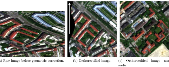
(a) Raw image before geometric correction. (b) Orthorectied image. (c) Orthorectied image near nadir.
Figure 2.3: Geometric distortions of an optical RS image. An image before (Figure 2.3a) and after (Figures 2.3b and 2.3c) the orthorectication process. The image was acquired by the HySpex sensor, an air-borne push-broom HSI sensor with 34◦FOV. The white arrow points into the ight direction. Figure 2.3b shows a geometrically corrected detail from the border of a scan line, where façades of the buildings caused by inaccurate DSM are still partially seen. This can be observed in as white areas on building boundaries. This eect is not seen in an image from the central part of the scan line, where the viewing angle is looking nearly at nadir (Figure 2.3c).
For systems with whisk- or push-broom acquisition technology, every pixel of an image in across-track direction is collected at a dierent viewing angle. On a rugged terrain surface two geometric distortions are dicult to correct due to this side-looking geometry and (in)accuracy of the model of the surface model required for the correction. First, named relief displacement is a shift in an object's position in an image due to the object's height above (or below) ground and viewing direction of the sensor.
Let us assume an accurate and error free model of a terrain surface, e.g. DSM, is available for relief displacement correction. If this DSM is not precisely registered to the image, which exhibits rugged terrain, the correction will also cause relief displacement. The relief displacement is caused also by inaccurate DSM. Second, the high-rise objects are imaged from a side, and might obstruct the sensor view on other objects. The occlusion areas are interpolated in the correction process, whereas the sides of the objects can still be partially seen in a corrected image (Figure 2.3b). These two inuences are larger on the extremities of the scan line and are not present at the nadir or on at terrain. They are more prominent for higher objects and for sensors with larger FOV.
2.2 Digital Elevation Models
2.2.1 Terminology
Digital Surface Model (DSM) is a digital representation of terrain surface and all objects on it, e.g.
buildings and trees, whereas Digital Terrain Model (DTM) is a digital representation of a surface without objects on it. The normalised Digital Surface Model (nDSM) exhibits only the heights of the objects above ground, and can be described by a simplication subtraction of DTM from DSM. The term Digital Elevation Model (DEM) is used as a generic term for all digital surface representations.
The DEM dened by height values for a selected set of planar coordinates are also referred to as 2.5D DEM. The height, also called elevation is measured with respect to a hight reference point or surface. They can be represented by a regular grid, i.e. raster, by an irregular grid such as triangular irregular network, or point clouds. The terms DEM, DSM, and DTM are used, when it is referred to the representation of terrain surface in a regular, equally spaced grid. Three common data types to generate DEM are stereo optical images, LiDAR point clouds (Subsection 2.2.2) and Synthetic Aperture Radar (SAR) images. The accuracy of the input data, as well as the method for DEM generation inuence the accuracy of the DEM.
The surface model, most often a gridded DEM, is a necessary input for orthorectication of all op- tical RS imagery. Its accuracy and errors inuence the radiometric and geometric accuracy of the orthorectied image (Section 2.1).
2.2.2 DEM Generation and Their Characteristics
The DEM can be generated from air- or space-borne RS data or terrestrial measurements. The latter are due to the high acquisition costs seldom used for larger areas and are not further discussed. In the following Subsections, methods, acquisition principles, and possible sources of errors of the DEM from stereo optical imagery and LiDAR point cloud acquisition are discussed. Alternatively, the DSM (also of a larger coverage) can be generated by means of interferometric SAR.
Dense-Matching
Stereo matching is one of the most active research areas in the eld of computer vision and photogram-
metry (Scharstein and Szeliski, 2002). The descriptions here are focused on the dense stereo matching
(a) SGM DSM from 3K images with holes. (b) Semi-Global Matching (SGM) DSM from 3K images without holes and smoothed with median lter.
(c) SGM DSM from WV-2 images. (d) RGB composite image of the urban area.
Figure 2.4: DSM of an urban area (Figure 2.4d) computed using SGM method. The SGM DSM (Figure 2.4a) is calculated from stereo images acquired by the 3K camera system (see Subsection 6.1.2, p.82 for details). Missing values (holes) are lled and the DSM is smoothed with a median lter (Figure 2.4b). Figure 2.4c shows SGM-DSM from WorldView-2 (WV-2) images. The pixel size of 3K DSM is 0.3 m (Figures 2.4a and 2.4b), and the pixel size of the WV-2 DSM is 0.5 m (Figure 2.4c). All DSM are colour coded from low (black) to high (white).
methods with known camera geometry and their application to the 3D surface model computation.
The DSM from stereo imagery used in this thesis are computed by Semi-Global Matching (SGM) method described below.
A prerequisite for DEM computation are at least two images of the same scene (object) taken from
dierent directions. First, the correspondence between the images is found for every pixel in an image
based on their intensity values, i.e. area correlation methods. Alternatively, the correspondence can be
based on extracted features such as Scale-Invariant Feature Transform (SIFT) features, or combination
of area and feature based methods. Second, the depth map is computed, where each pixel in the depth
map contains the value of the distance between the camera centre to the corresponding 3D point in the
scene. Dense depth maps are a result of the area correlation methods, in contrast to the sparse depth
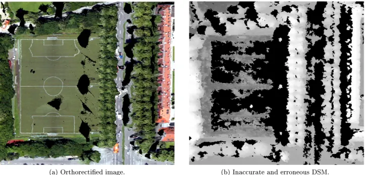
(a) Orthorectied image. (b) Inaccurate and erroneous DSM.
Figure 2.5: Orthorectied view of the nadir image of the 3K camera (Figure 2.5a). It is orthorectied with erroneous DSM with holes (Figure 2.5b, black areas). The holes in DSM are due to the texture-less areas on the football eld and red roofs, occlusions, etc.
maps, which are a result of matching only features (Veksler, 2001). Finally, the DEM is computed by projecting the depth map using camera geometry into the map coordinate system. Errors in dense stereo matching DEM can occur due to repetitive textures (patterns), texture-less regions, shadows and low contrast regions, specular reection (e.g. glass, solar panels), clouds, haze, occlusions of the objects or invisible parts of scene, and moving objects, e.g. cars, people (Hirschmüller, 2005; Scharstein and Szeliski, 2002; Veksler, 2001).
The SGM algorithm is one of the dense stereo matching methods, which performs pixel-wise matching and approximation of the 2D smoothness constraint (Hirschmüller, 2005). This method is robust against illumination changes and accurate on the boundaries of an object when appropriate smoothing term for pixel-wise matching is chosen. Nevertheless, some holes in the DEM mainly due to occlusions, texture-less, and low contrast regions might still occur. In postprocessing steps, these holes can be interpolated or lled from existing DEM of the same area. Additionally, a whole DEM can be smoothed by e.g. median lter to remove possible outliers. Note that any smoothing or interpolation of the data introduces some inaccuracies to the DEM. Even though SGM performs well on the boundaries of objects, a typical SGM DEM of high-rise object areas still exhibits wave-like shaped boundaries of buildings (Figure 2.4), due to the smoothness constraint.
LiDAR Point Cloud
The basic principle of a LiDAR system is the determination of the distance of a target by emitting pulses of a laser light and measuring the time of arrival of the reected light. Moreover, the LiDAR sensors record also the intensity of the backscattered light. Air-Borne Laser Scanner (ALS) systems are mounted on air-borne platforms and include LiDAR system as well as other instruments, e.g. Global Navigation Satellite System (GNSS)/Inertial Navigation System (INS) unit for attitude determination.
For RS applications such as topographic mapping, the LiDAR systems, which emit the pulses in NIR
spectrum (usually between 1.040-1.065 µ m), are used (Gatziolis and Andersen, 2008). There are two
types of LiDAR sensors according to the quantication of the recorded backscattering light. First,
(a) ALS point cloud (2.3 points/m2). (b) Interpolated LiDAR point cloud.
Figure 2.6: First response LiDAR point cloud (Figure 2.6a, green-low, red-high) and DSM interpolated from this LiDAR point cloud by bilinear method (Figure 2.6a). The average point density of the LiDAR point cloud is about 2.3 points/m2, and is interpolated to the 0.3 m gridded DEM. A zoomed-in point cloud demonstrates the eect of the planar error of the points on a boundary of a high-rise object. This error together with the irregular scanning pattern is propagated to the interpolated LiDAR DSM and can be observed as zig-zag pattern on the boundaries of high-rise objects (Figure 2.6b).
so called full waveform LiDAR sensors that record the reected light nearly continuously. Second, the discrete-return LiDAR sensors that record the backscattered light at dened intervals, e.g. as a rst (Figure 2.6a) and last return. The points in the LiDAR point cloud are not regularly spaced, in comparison to the DEM computed by the dense stereo matching methods. However, the LiDAR point clouds can be interpolated to a regular grid by e.g. polynomial interpolation, inverse distance weighting, kriging, and are referred to as LiDAR DEM.
Two main categories of errors of the LiDAR point cloud are elevation and horizontal errors. The measured elevation error can occur due to the sensor system and platform characteristics, e.g. analysis of the waveform, identication of the return position, pulse length, and position error measured by the GNSS/INS unit. The horizontal error has its main sources in ying height accuracy and reections from the sloped surface (Hodgson and Bresnahan, 2004). Even if the distance from a sensor to a sloped surface is measured without an error, the planar error of such measured response introduces an apparent systematic error in the measured distance. This error has a similar behaviour like the relief displacement in optical imagery and is most prominent on the boundaries of high-rise objects. The zoomed in area in Figure 2.6b demonstrates this eect. The gridded LiDAR DEM include additionally the interpolation error.
2.3 Image Fusion in Urban Areas
Image fusion is a process of integrating two or more images and/or their inherent information into a
single output, which includes enhanced desired information content compared to any of the input
images. The objective of the image fusion and therefore desired information content of the fused
result is highly dependent on the application (Chaudhuri and Kotwal, 2013, p.1920). A prerequisite
for any image fusion is a good coregistration between all the used datasets.
Urban areas exhibit large variety of objects on a relative small area, which vary in material, texture, height, shape, size, etc. Therefore, image fusion from multi-modal sensors is a necessity to enable or improve the robustness and accuracy of extracted information about urban areas (Gamba, 2014).
There are numerous ways to classify image fusion techniques, for example according to
domain, e.g. spatial or frequency domain,
resolution, e.g. resolution enhancement method such as spectral enhancement of MS image by using lower-spatial resolution HSI,
modality also called multi-sensor, e.g. fusion of MS images, DEM, and HSI,
acquisition time also called multi-temporal, e.g. images of the same area acquired at dierent times, often used for change detection, and
processing level: pixel-, object-, and decision-based methods, or pixel- and feature-based methods.
The main aim of photogrammetry regarding the urban environment is to model it in 3D with all the characteristics (Brook et al., 2013), for instance as proposed by CityGML Standard (Gröger et al., 2012;
Gröger and Plümer, 2012). The built urban environment comprises the 3D objects in it. Therefore, many data fusion methods modelling urban environment use height data, e.g. DEM or LiDAR point clouds, next to at least one more dataset of dierent modality.
2.3.1 Availability of the Multi-View and Hyperspectral Images
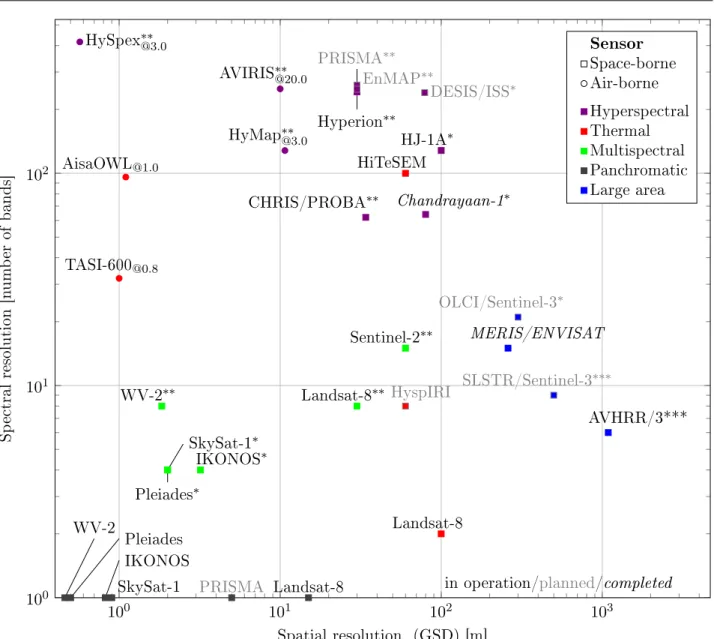
The availability and coverage of the data from stereo- and multi-view optical imagery has increased due to a larger number of air- and space-borne platforms carrying high spatial resolution cameras (Figure 2.7), e.g. WV-2, Pleiades, UltraCam. Next to these sensors, also the HSI sensors with higher spectral, but in comparison to MS imagery lower spatial resolution exist or are planned for EO missions.
The main trend in EO optical sensors is going towards development of even higher spectral resolution (HSI) sensors, as well as into the direction of a larger number of lower-cost eet of satellites, e.g. SkySat by SkyBox Imaging. Another direction of development is the area of low-cost optical systems carried on unmanned aerial platforms.
2.3.2 Potential and Challenges of the HSI and DSM Fusion
The main potential of HSI and DEM fusion for urban areas originates from dierent modality and characteristics of the images. The HSI enable e.g. material identication, the DSM the height char- acterisation of the objects, and both image types carry information about the objects. The fusion of these two data types includes applications for identication of the 3D objects in the scene from DSM and assignment of the material properties to these objects, detecting potentially dangerous materials, and/or change of the materials, and classication based on spectral, spatial, and/or geometric features.
In view of building extraction from HSI and DSM, the inuences of the geometric distortions and data characteristics are addressed in the following paragraphs.
The orthorectied HSI rarely include information of the used DSM, its accuracy, and coregistration error. Even if the accuracy of the DEM is given, it might vary signicantly within the same dataset.
Such an example are lines of a soccer eld in Figure 2.5, which vary from nearly straight to very curvy
lines, due to the erroneous DSM used for orthorectication. The marks on the soccer eld, boundaries
of the streets, and the building outline should be straight lines, but appear as lines with dierent
curvatures. The wavy right boundary of the building on the right is mainly due to the wavy shape
of the DSM. On the left, the building boundary is wrongly projected due to the large hole in the
100 101 102 103 100
101 102
Hyperion
∗∗PRISMA∗∗
SkySat-1
∗Pleiades
∗WV-2 Pleiades IKONOS
in operation/planned/completed CHRIS/PROBA
∗∗HJ-1A
∗Chandrayaan-1
∗ EnMAP∗∗DESIS/ISS∗
HySpex
∗∗@3.0HyMap
∗∗@3.0AVIRIS
∗∗@20.0HiTeSEM
Landsat-8
HyspIRIAisaOWL
@1.0TASI-600
@0.8Sentinel-2
∗∗Landsat-8
∗∗WV-2
∗∗IKONOS
∗PRISMA
Landsat-8 SkySat-1
AVHRR/3***
MERIS/ENVISAT
OLCI/Sentinel-3∗SLSTR/Sentinel-3∗∗∗
Spatial resolution (GSD) [m]
Sp ectral resolution [n um ber of bands]
Sensor Space-borne Air-borne Hyperspectral Thermal Multispectral Panchromatic Large area
Figure 2.7: Spectral resolution as a function of spatial resolution for selected EO air- (circular marker) and space-borne (square marker) sensors. Colour of a marker denotes a type of a sensor, i.e. violet for HSI, red for TIR, green for MS, dark grey for Panchromatic (PAN), and blue for large area assessment sensors. A black text of a sensor/platform is for operational, grey text for planned, and black italic text for completed missions as of autumn 2015. The portion of observed spectrum by HSI and MS sensors is denoted by ∗for VNIR, ∗∗ for VNIR and SWIR, and∗ ∗ ∗ for VNIR, SWIR, and TIR. The spatial resolution of air-borne sensors is given for a certain ight height (@height in km) as given in producer's specications.
DSM. A DSM for orthorectication of a HSI and a DSM used for fusion with the HSI are in general case not the same. The reason for this is that the ordered orthorectied, e.g. satellite images, are not delivered together with the DSM used for orthorectication. Thus, the inaccuracies of the HSI due to orthorectication are not dependent on or caused by the inaccuracies and errors in the DSM for orthorectication.
The decreased planar and spectral accuracy in HSI is expected on the boundaries of high-rise objects,
because of the instrumental and processing inuences (Subsection 2.1.2). Similarly, the decreased
planar and height accuracy of DSM is expected on the boundaries of the same high-rise objects (Sub-
section 2.2.2). Moreover, imprecise registration of the datasets causes errors on the boundaries of these
objects. Thus, these inaccuracies in HSI and DSM occur on the boundaries of the same high-rise
objects. Other partially or not corrected systematic errors are not expected on the same parts (i.e.
boundaries) of these objects in the images. Let us take for example a SGM DSM with higher spatial
resolution than HSI and a HSI captured by a sensor with a narrow FOV (this means the eect of relief
displacement is limited). The DEM can have holes on texture-less areas such as uniform roofs, but the
spectral and spatial characteristics of the same roof are still well captured by the HSI sensor. If the
DSM is well modelled, the outline of a high-rise object can be better extracted from the higher spatial
resolution DSM than from HSI. The fusion of HSI and DSM can support extraction of the objects
and make it more robust. It is however not limited to the extraction of material and height features
from HSI and DSM respectively, but has also a potential to improve the boundary extraction of these
objects.
3 Advances in HSI and DSM Fusion for Building Extraction
Building extraction and modelling is an active research eld for urban object detection from RS imagery (Rottensteiner et al., 2012), followed by road (Mena, 2003) and urban vegetation extraction (Mayer, 2008; Rottensteiner et al., 2014). Two main reasons for this are the variety of applications, which require building models or outlines as input, and lack of fully operational methods for building extraction, their transferability, and/or sucient quality. Moreover, urban areas are continuously undergoing changes, which require cost-ecient updates of the spatial databases.
The objective of this Chapter is to give the state of the art about building extraction from RS data, which follows a common workow. A special focus is on multi-modal datasets and 2D building outline extraction and adjustment with sub-pixel precision. A building outline is described by a polygon, which can be derived from extracted line segments and edges. In view of applicability of scale space edge detection on RS imagery, a broader overview of RS methods using scale space is given. Finally, the diversity of evaluation techniques for building extraction is summarised and the reasoning for further developments in this thesis is given.
3.1 Building Extraction from Remote Sensing Data
Object extraction, as understood in this thesis, is based on modelling of a 2D or 3D object by geometric description and optional extraction of additional attributes like semantic and topological information (Baltsavias, 2004). The modelling (i.e. polygon description) of objects means that the modelled object (i.e. extracted polygon) has signicantly reduced number of vertices in comparison to the data points describing object's boundary in the original dataset (Wang, 2013), while maintaining its geometrical characteristics. For example, connected boundary pixels of a building region from a raster image (Vu et al., 2009) or Triangulated Irregular Network (TIN) of the building data points are not considered as geometrical building modelling, even if they are vector representations of an object.
Building extraction methods can be divided into data- and model-driven methods (Heuel and Kolbe, 2001; Tarsha-Kurdi et al., 2007; Vosselman and Maas, 2010), or hybrid versions of both approaches.
The data-driven methods rely on low-level features and shapes, and combine them into a building polygon in a bottom-up manner, for instance constructing a model of a building boundary from a set of rectangles (Are, 2009; Avbelj et al., 2013a, 2015a; Gerke et al., 2001; Kwak and Habib, 2014).
Model-driven methods t a parametric model from a given library or set of models and select the best tting one. The advantages of model-driven approaches are computational eciency and robustness.
Furthermore, the topological relations and constraints between the polygon edges must not be modelled, because they are included in the library of models. However, the disadvantages of such approaches are inexibility, and inability to model complex objects not included in the library. If only few data points per object are available, i.e. the spatial resolution of the image is relatively low in comparison to the object extent, the model-driven approaches outperform the data driven ones (Henn et al., 2013).
The methods for automatic building extraction can be grouped according to the modality of the data.
Some example works are give as follows:
Optical images: PAN (Lin and Nevatia, 1998), MS (Lee et al., 2003), and HSI.