IWR, University of Heidelberg Winter term 2015/16
Exercise Sheet 8 10. December 2014
Exercise for Course
Parallel High-Performance Computing Dr. S. Lang
Return: 17. December 2014 at the beginning of the exercise or earlier
Task 17 MPI: Communication in the ring (5 points)
With this task we want to perform first steps with MPI. Implement a communication of 8 processes in the ring. Each process shall sent its rank within a message once in the ring and terminate, if it again receives its rank within a message. Use synchronous sending resp. receiving and one of the techniques presented in the lecture, to avoid deadlocks, e.g. coloring of the edges. Each process shall in each send/receive step print its ranks and the just received message. Test your program in the pool and hand in an output of the communication sequence.
More details for using of MPI in the pool is on the Homepage. Helpful for the right syntax are the manpages about MPI (e.g.man MPI_Comm_rank).
Task 18 Parallel Computing of π with MPI (5 points)
From the identity π = 4(arctan 1) one gets by usage of the derivative of the arctan, (arctanx)0
= 1/(1 +x2), a formula for calculating π:
π= Z 1
0
4 1 +x2dx.
By division of the interval into n equidistant partial pieces the integral can be evaluated with the midpoint rule. You can find a sequential program in the file piseq.c on the homepage. We want to parallelize it with MPI. The strategy is:
• process 0 reads the number of partial intervals and passes it to all other processes,
• Theforloop over the partial intervals will be parallelised, each process calculates a local partial sum. The results wil be collected by process 0 with a reduction operationMPI_Reduce and the partial sums are added.
First determine the convergence order of the midpoint rule with the sequential program. Establish a double-logarithmic plot with the integration error over the interval lengthh. The steepness of the line give the order. Now implement a parallel version. Compare the accuracy in the calculations (last digits) with the sequential solution and the exact value (short discussion).
Optional task additional 5 credit points
The number of valid digit positions can be enhanced by using the Gnu Multiprecision Arithmetic Library (GMP, you can find at www.gmplib.org, for the most Linux distributions there is a package).
Thus π could be calculated e.g. up to 40., 60. or 80 positions. Of course the choosen method with quadratic convergence is much to slow for that, this means a up to 80.digit exact program would run nearly forever. Implement a version of the sequential or parallel program, that uses the GMP. If you want to gain high accuracy, you need to use a better method than the midpoint rule. Otherwise you can test which accuracy you can achieve with GMP and the midpoint rule in a meaningful computing time. You can get the reference value ofpi by internet.
Task 19 Simple Parallelisation of the Jacobi method with MPI (10 points) For linear equation systemsAx=b, A∈Rn×n,x,b∈Rn,n∈N, direct solution methods are mostly inefficient for largen. Therefore one often uses iterative methods like theJacobi method. You get the
method by additive spliting of the system matrixA in an upper and low triangular matrix U and L and the diagonal matrixD,A=D+L+U. This leads to the fixpoint iterationx=D−1(b−(A−D)x), that can be solved under certain circumstances:x(m+1) =D−1(b−(A−D)x(m)), Indexm∈Nis the iteration step. Thei.th equation for the (m+ 1). step of the method is then called
x(m+1)i = bi−P
j6=iaijx(m)j aii
.
As starting vectorx0 you can use each arbitrary vector. The calculation of the residual rprovides a termination condition in m.th step. rm := b−Ax(m): Is an adequate norm of the residual (e.g. the maximum norm||r||∞) smaller than a given tolerance ∈R+, the iteration stops. The calculation of the iteration depend only on the previous solution and therrre are no data dependencies between the newly calculated values xi. Thus the Jacobi methods is easy to parallelize.
We want to use the Jacobi method, to calculate the discrete solution of the poisson equation
− 4u=f in Ω = (0, r)2, u= 0 auf ∂Ω
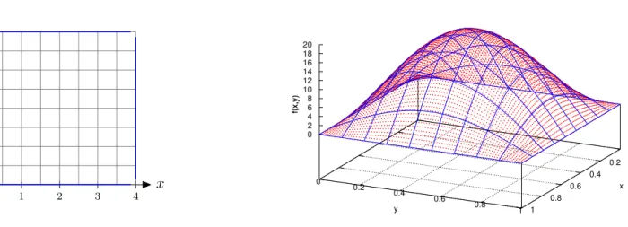
on a square with side length r. The source f be f(x, y) := 2π2sin(πx)·sin(πy). Then the analytic solution is given byu(x, y) = sin(πx)·sin(πy). The unit square is covered from a grid withn2 points, see Figure 0.5 left withr= 4 andn= 9. The distancehbetween two points (the
”grid resolution“) is h=r/(n−1). In the Figure to the right a source f is shown.
An equation system in matrix shape is gotten by approximation of the second derivative through a central difference quotient at each inner grid point (i, j) mit i, j = 1. . . n−1. At the boundary points with i= 0 or i=n(also for j) the solution is predefined. The grid points can be enumerated consecutively byk=i·n+j, thus each index pair (i, j) is mapped onto an index k in a unique way.
Then we can consider the grid function
uh := (u01, u02, . . . , u0n, u11, . . . , u1n, . . . , un1, . . . unn)T = (u1, . . . uN)T
withN =n2. After the approximation of the second derivative the equation system for the unknown grid function uh (details to the derivation soon) reads:
1 h2
4 −1 · · · −1
−1 4 −1 · · · −1 . .. ... ... . ..
. .. −1 . ..
−1 4 −1 · · · −1
−1 . ..
. .. −1
· · · −1 4
N×N
·
u0
... ... ... ... ... ... uN
=
f0
... ... ... ... ... ... fN
.
The valuesf1 tofN are evaluations of the sourcef at the grid points. Each line correspoinds to a grid point xii. The matrix contains on the diagonal the 4 as entry ofuii, and in the direct neighbors left and right the entry−1 at the indicesui−1j and ui+1j. Furthermore there are in each row two further entries−1. This are exactly the one of the neighbors above and belowuij+1 anduij−1. Therefore the distane between the −1 right beneath a 4 and the next −1 justn.
At a boundary point the assigned matrix line has to be substituted through a null line with a 1 on the diagonal entry, the solutionu has to be set in this case to 0 as well as the right side also to 0.
Task
1. Develop a MPI-parallel variant of the Jacobi method. A possible strategy is to split the matrixA and the vectors in stripes of size (row or column count)α, each processor works with one stripe.
x y
0 1 2 3 4
0 1 2 3 4
0 0.2 0.4 0.6 0.8 1
0 0.2
0.4 0.6
0.8 1
0 2 4 6 8 10 12 14 16 18 20
f(x,y)
Numerical, n=80 Analytical
x y
f(x,y)
Abbildung 0.5: Left: area Ω with discretization, right: sourcef(x, y).
Each processor gets in the Jacobi step m a copy of the previous solution x(m−1), to calculate the new values xi of a stripe. Then in each iteration each process hat to communicate its new values of its partial domain to all other processes, e.g. using multi broadcast.
2. Initialize the initial solution uh with 0.0. Set r = 1.0 and use a tolerance for = 10−4. Don’t forget when assembling the matrix and the initialisation of the vectors the treatment of the boundary points! Test with your code the convergence of the errorku−uhk∞ between analytic uand numerical solutionuh at the grid points forn= 4,8,16,32 and 64. Establish a plot of the error over the grid widthh. Can you determine the consistency order?
3. Measure the speedup in the pool against the sequential version (P = 1) for different problem sizesn≤32 and processor countsP.
Hints
• If you like you can implement another strategy, that you can find in a textbook on numerical solution methods for linear equation systems.
• If you have any difficulties you can make the task easier and choose a another matrix without physical application. For convergence of the Jacobi method the matrix A needs to be strictly diagonal dominant: It should apply for each linePn
j=1;j6=i|aij|<|aii|,∀i∈ {1, .., n}(the absolute value of diagonal element of each line should be greater than the sum of absolute values of the off diagonal entries).