Determination of Sub-daily Earth Rotation Parameters from VLBI Observations

Deutsche Geodätische Kommission der Bayerischen Akademie der Wissenschaften

Reihe C Dissertationen Heft Nr. 765

Thomas Artz

Determination of Sub-daily Earth Rotation Parameters from VLBI Observations

München 2016

Verlag der Bayerischen Akademie der Wissenschaften in Kommission beim Verlag C. H. Beck

ISSN 0065-5325 ISBN 978-3-7696-5177-5

Diese Arbeit ist gleichzeitig veröffentlicht in:

Schriftenreihe des Instituts für Geodäsie und Geoinformation der Rheinischen Friedrich-Wilhelms Universität Bonn

ISSN 1864-1113, Nr. 47, Bonn 2011

Deutsche Geodätische Kommission der Bayerischen Akademie der Wissenschaften

Reihe C Dissertationen Heft Nr. 765

Determination of Sub-daily Earth Rotation Parameters from VLBI Observations

Inaugural-Dissertation zur Erlangung des Grades Doktor-Ingenieur (Dr.-Ing.) der Hohen Landwirtschaftlichen Fakultät der Rheinischen Friedrich-Wilhelms Universität

zu Bonn

vorgelegt am 05.09.2011 von

Dipl.-Ing. Thomas Artz

aus Wesel

München 2016

Verlag der Bayerischen Akademie der Wissenschaften in Kommission beim Verlag C. H. Beck

ISSN 0065-5325 ISBN 978-3-7696-5177-5

Diese Arbeit ist gleichzeitig veröffentlicht in:

Schriftenreihe des Instituts für Geodäsie und Geoinformation der Rheinischen Friedrich-Wilhelms Universität Bonn

ISSN 1864-1113, Nr. 47, Bonn 2011

Adresse der Deutschen Geodätischen Kommission:

Deutsche Geodätische Kommission

Alfons-Goppel-Straße 11 ! D – 80539 München

Telefon +49 – 89 – 230311113 ! Telefax +49 – 89 – 23031-1283 /-1100 e-mail hornik@dgfi.badw.de ! http://www.dgk.badw.de

Diese Publikation ist als pdf-Dokument veröffentlicht im Internet unter den Adressen / This volume is published in the internet

<http://dgk.badw.de> / <http://hss.ulb.uni-bonn.de/2011/2710/2710.htm>

Prüfungskommission

Referent: Priv.-Doz. Dr.-Ing. Axel Nothnagel Korreferenten: Univ.-Prof. Dr.-Ing. Heiner Kuhlmann

Univ.-Prof. Dr.-Ing. Dr. h.c. Harald Schuh Tag der mündlichen Prüfung: 14.10.2011

© 2016 Deutsche Geodätische Kommission, München

Alle Rechte vorbehalten. Ohne Genehmigung der Herausgeber ist es auch nicht gestattet,

die Veröffentlichung oder Teile daraus auf photomechanischem Wege (Photokopie, Mikrokopie) zu vervielfältigen

ISSN 0065-5325 ISBN 978-3-7696-5177-5

Determination of Sub-daily Earth Rotation Parameters from VLBI Observations

Summary

The work presented deals with the determination of sub-daily Earth Rotation Parameters (ERPs) from Very Long Baseline Interferometry (VLBI) observations. Monitoring and interpreting the Earth’s rotation variations in general is an important task for Earth sciences, as they provide boundary which support other geophysical investigations. This holds especially for sub-daily variations of the Earth’s rotation which are primarily excited by variations of the oceans. Furthermore, atmospheric impacts as well as effects of the shape of the Earth are present. VLBI observations are in particular feasible. With VLBI all five parameters of the Earth’s orientation can be determined without hypothesis. Thus, VLBI derived results do not suffer from resonance effects from the modeling of artificial Earth satellites, which is the fact for ERPs derived, e.g., from observations of Global Navigation Satellite Systems (GNSS).

Although the analysis of sub-daily variations of the Earth’s rotation is by no means a new scientific area of research, there is a clear need to expand the methods used. This is also obvious as further studies by other authors were performed in parallel to the results presented in this thesis. Thus, the determination and analysis of sub-daily ERPs can be considered as a vital field of research. The determination of sub-daily ERPs from VLBI observations can be divided into two areas. On the one hand, time series with a high temporal resolution, e.g., one hour, can be generated. On the other hand, an empirical model for the tidal variations of the ERPs with periods of one day and below can be determined from the VLBI observations.

Both areas of research are considered within this thesis.

Concerning the time series approach, special continuous VLBI campaigns are examined as they offer ideal conditions for this approach. For the analysis of these campaigns, an optimized solution scheme is imple- mented. This adapts the continuous character in an optimal way and avoids negative influences of the VLBI-analysis on the subsequent examination of the sub-daily ERPs. In this way, irregular variations are confirmed and further ones are detected. However, it is pointed out that these variations can be confirmed only with continuous campaigns over longer time spans. Furthermore, a temporal resolution below one hour of the sub-daily ERPs would be desirable to detect additional short periodic variations. This is not possible with the current status of VLBI observations, but, improvement is promised by future technical concepts of VLBI. The analysis methods that are applied within this thesis, will be directly applicable to future VLBI observations.

With regard to the determination of an empirical model for tidal ERP variations, a new methodology

based on the transformation of normal equation systems is developed. It is shown that this approach can

be successfully applied to VLBI observations. Moreover, this approach provides a straight forward method

for the combination of different space-geodetic techniques, being the most rigorous one known today, when

different software packages are used to pre-process the individual techniques. Within the thesis at hand, the

approach of the transformation of normal equation systems is used to estimate an empirical model for tidal

ERP variations from observations of the Global Positioning Systems (GPS) as well. On this basis, the work

of this thesis cumulates in a rigorous combination of GPS and VLBI observations. The combined time series

with an hourly resolution as well as the determined empirical model for tidal ERP variations exhibit that

the strengths of both techniques are sustained.

Bestimmung von subtäglichen Erdrotationsparametern aus VLBI Beobachtungen

Zusammenfassung

Die vorliegende Arbeit befasst sich mit der Bestimmung subtäglicher Erdrotationsparameter (ERP) aus Beobachtungen der Radio-Interferometrie auf langen Basislinien (engl.: Very Long Baseline Interferometry, VLBI). Die Beobachtung und Interpretation der Erdrotation im Allgemeinen stellt einen wichtigen Schwer- punkt der Erdwisschenschaften dar, da sie Randbedingungen für andere geowissenschaftliche Untersuchungen setzt. Dies gilt im Speziellen auch für subtägliche Variationen der Erdrotation. Diese sind vor allem bedingt durch Variationen des Ozeans, darüberhinaus lassen sich Effekte der Atmosphäre, wie auch der Gestalt der Erde feststellen. Die Beobachtungstechnik VLBI eignet sich im Besonderen für Untersuchungen der Erdrota- tion, da einzig mit dieser Technik alle fünf Parameter der Erdorientierung hypothesenfrei bestimmt werden können. Somit sind im Gegensatz zu Ergebnissen, die z.B. aus den Beobachtungen globaler Satellitennavi- gationssysteme (engl. Global Navigation Satellite System, GNSS) gewonnen werden, keine Resonanzeffekte aus der Modellierung künstlicher Erdsatelliten zu erwarten.

Obwohl die Untersuchung subtäglicher Erdrotationsvariationen keineswegs ein neuartiges wissenschaftliches Forschungsgebiet darstellt, besteht doch ein eindeutiger Bedarf bezüglich der Erweiterung der auf diesem Ge- biet verwendeten Methoden. Dies wird auch daran deutlich, dass parallel zu den in dieser Arbeit dargestellten Ergebnissen weitere Untersuchungen anderer Autoren erfolgten und es sich somit um ein vitales Forschungs- gebiet handelt. Die Bestimmung subtäglicher ERP aus VLBI-Beobachtungen lässt sich in zwei Teilgebiete aufgliedern. Zum Einen können Zeitreihen mit hoher zeitlicher Auflösung von beispielsweise einer Stunde generiert werden. Zum Anderen kann ein empirisches Modell für die gezeitenbedingten Variationen der ERP mit Perioden von einem Tag und weniger aus den VLBI-Beobachtungen geschätzt werden. Beide Forschungszweige sind Bestandteil dieser Arbeit.

Bezüglich des Zeitreihenansatzes werden spezielle kontinuierliche VLBI-Kampagnen untersucht, da sie die idealen Voraussetzungen für diesen Ansatz bieten. Zur Analyse dieser Kampagnen wird ein Lösungsschema entwickelt, welches optimal auf den kontinuierlichen Charakter angepasst ist. Dadurch werden negative Ein- flüsse der VLBI-Auswertung auf eine anschließende Untersuchung der subtäglichen ERP-Zeitreihen min- imiert. Es wird gezeigt, dass sich bereits entdeckte irreguläre Variationen bestätigen und weitere detektieren lassen. Allerdings wird ebenso deutlich, dass diese Variationen nur mit kontinuierlichen Kampagnen über län- gere Zeiträume bestätigt werden können. Darüber hinaus wäre eine zeitliche Auflösung der ERP-Zeitreihen von deutlich unter einer Stunde wünschenswert, um weitere kurzperiodische Signale zu detektieren. Dies ist mit dem aktuellen Stand der geodätischen VLBI allerdings nicht möglich, zukünftige Entwicklungen ver- sprechen jedoch deutliche Verbesserungen in dieser Hinsicht. Die in der vorliegenden Arbeit angewendeten Analysemethoden werden direkt auf die Analyse zukünftiger VLBI-Beobachtungen anwendbar sein.

Im Hinblick auf die Bestimmung eines empirischen Modells für ERP-Variationen wird im Rahmen dieser Arbeit eine neue Methodik entwickelt, die auf der Transformation von Normalgleichungssystemen basiert.

Es wird nachgewiesen, dass sich dieser Ansatz erfolgreich auf VLBI-Beobachtungen anwenden lässt. Außer-

dem gewährleistet der Ansatz eine einfach zu realisierende Kombination verschiedener weltraumgeodätischer

Verfahren, die zudem den strengsten zur Zeit realisierbaren Ansatz darstellt, so lange verschiedene Soft-

warepakete zur Vorprozessierung der einzelnen Techniken verwendet werden. Im Rahmen der vorliegenden

Arbeit wird die Transformation von Normalgleichungssystemen ebenfalls zur Bestimmung eines empirischen

Modells für ERP-Variationen aus Beobachtungen des Global Positioning Systems (GPS) angewendet. Auf

dieser Basis erfolgt abschließend eine rigorose Kombination von GPS- und VLBI-Beobachtungen. Sowohl

die kombinierten ERP-Zeitreihen mit stündlicher Auflösung als auch das gewonnene kombinierte empirische

Modell für ERP-Variationen zeigen, dass die Kombination die Stärken beider Techniken nutzt.

5

Contents

Preface 7

1 Introduction 9

2 Scientific context 11

3 Theory of Sub-daily Earth Rotation 13

3.1 Earth Orientation Parameters . . . . 13

3.2 Excitation of the Earth Rotation Parameters . . . . 16

3.2.1 UT1 and Length-of-Day Variations . . . . 17

3.2.2 Polar Motion . . . . 19

4 Measuring Earth Rotation Parameters with VLBI 21 4.1 The Basic Principle of VLBI . . . . 21

4.2 Parameter Estimation . . . . 23

4.3 Determination of Earth Rotation Parameters . . . . 25

4.3.1 Estimating Time Series of Highly Resolved Earth Rotation Parameters . . . . 26

4.3.2 Estimating an Empirical Model for Tidal Variations of the Earth Rotation Parameters 27 5 Short description of the included papers 29 5.1 Main Points of Paper A . . . . 29

5.2 Main Points of Paper B . . . . 30

5.3 Main Points of Paper C . . . . 30

5.4 Main Points of Paper D . . . . 30

5.5 Main Points of Paper E . . . . 31

5.6 Main Points of Paper F . . . . 31

5.7 Main Points of Paper G . . . . 32

6 Summary of the most important results 33 6.1 Analysis of Continuous VLBI Campaigns . . . . 33

6.2 An Empirical Tidal Model for Variations of the Earth Orientation Parameters from VLBI Observations . . . . 37

6.3 Inter-technique Combination to Estimate Sub-daily Earth Orientation Parameters . . . . 42

6.3.1 Long Term Time Series . . . . 43

6.3.2 Impact of various VLBI observing session types . . . . 45

6.3.3 Empirical Model for Tidal Variations of the Earth Orientation Parameters . . . . 46

6 Contents

7 Summary and Outlook 49

8 List of publications relevant to the thesis work 51

Abbreviations 53

List of Figures 54

List of Tables 55

References 57

A Appended Papers 69

A.1 Paper A . . . . 71

A.2 Paper B . . . . 73

A.3 Paper C . . . . 75

A.4 Paper D . . . . 77

A.5 Paper E . . . . 79

A.6 Paper F . . . . 81

A.7 Paper G . . . . 83

7

Preface

This thesis includes the following papers, ordered chronologically and referred to as Paper A – G in the text:

Paper A:

Artz, T., S. Böckmann, A. Nothnagel, V. Tesmer (2007) ERP time series with daily and sub- daily resolution determined from CONT05. In: Boehm, J., A. Pany, H. Schuh (eds) Proceedings of the 18th European VLBI for Geodesy and Astrometry Working Meeting, 12 – 13 April 2007, Vienna, Geowissenschaftliche Mitteilungen, Heft Nr. 79, Schriftenreihe der Studienrichtung Vermessung und Geoinformation, Technische Universität Wien, ISSN 1811-8380, pp 69 – 74, (available electronically at http://mars.hg.tuwien.ac.at/~evga/proceedings/S31_Artz.pdf).

Paper B:

Artz, T., S. Böckmann, A. Nothnagel (2009) CONT08 – First Results and High Frequency Earth Rotation. In: Bourda, G., P. Charlot, A. Collioud (eds) Proceedings of the 19th European VLBI for Geodesy and Astrometry Working Meeting, 24 – 25 March 2009, Bordeaux, Université Bordeaux 1 - CNRS - Laboratoire d’Astrophysique de Bordeaux, pp 111 – 115, (available electronically at http://

www.u-bordeaux1.fr/vlbi2009/proceedgs/26_Artz.pdf).

Paper C:

Artz, T., S. Böckmann, S., A. Nothnagel, P. Steigenberger (2010 a ) Subdiurnal variations in the Earth’s rotation from continuous Very Long Baseline Interferometry campaigns. J Geophys Res, 115, B05404, DOI 10.1029/2009JB006834.

Paper D:

Artz, T. S. Böckmann, L. Jensen, A. Nothnagel, P. Steigenberger (2010 b ) Reliability and Stability of VLBI-derived Sub-daily EOP Models. In: Behrend, D., K.D. Baver (eds) IVS 2010 General Meeting Proceedings “VLBI2010: From Vision to Reality”, 7 – 13 February 2010, Hobart, NASA/CP-2010-215864, pp 355 – 359, (available electronically at http://ivscc.gsfc.nasa.gov/publications/gm2010/artz.

pdf)

Paper E:

Artz, T., S. Tesmer, S., A. Nothnagel (2010 a ) Assessment of Periodic Sub-diurnal Earth Rotation Variations at Tidal Frequencies Through Transformation of VLBI Normal Equation Systems. J Geod, 85(9):565 – 584, DOI 10.1007/s00190-011-0457-z.

Paper F:

Artz, T., L. Bernhard, A. Nothnagel, P. Steigenberger, S. Tesmer (2011 b ) Methodology for the Combination of Sub-daily Earth Rotation from GPS and VLBI Observations J Geod, DOI 10.1007/s00190-011-0512-9, online first.

Paper G:

Artz, T., A. Nothnagel, P. Steigenberger, S. Tesmer (2011) Evaluation of Combined Sub-daily UT1

Estimates from GPS and VLBI Observations. In: Alef W., Bernhart S., Nothnagel A. (eds.) Proceedings

of the 20th Meeting of the European VLBI Group for Geodesy and Astrometry, Schriftenreihe des In-

stituts für Geodäsie und Geoinformation der Rheinischen-Friedrich-Wilhelms Universität Bonn, No. 22,

ISSN 1864-1113, pp 97 – 101.

9

1. Introduction

As the Earth is a continually changing planet, geodetic measurements are necessary to ensure increasing knowledge about the global change of the entire system Earth. The users of these geodetic products can be found in all areas where the knowledge of any object’s position is necessary. These are Earth sciences as well as societal applications, e.g., navigation and transport applications as well as early warning systems for natural hazards or weather forecasts.

Such fundamental geodetic products are the terrestrial and celestial reference frame (TRF and CRF) as well as the Earth Orientation Parameters (EOPs). The EOPs represent the rotational motion of the Earth by describing the rotational rate in terms of Universal Time (UT1) and by expressing the position of the instantaneous rotation axis with respect to (w.r.t.) the CRF (precession and nutation) and the TRF (polar motion, PM). Thus, the EOPs represent the link between TRF and CRF. The sub-group consisting of UT1 and PM is usually called Earth rotation parameters (ERPs). The rotational motion of the Earth exhibits variations on various time scales down to sub-daily phenomena which are forced by large-scale geophysical processes. These are external torques, mainly due to the gravitational attraction of the Sun and the Moon, as well internal dynamical processes. The latter can be separated into internal mass redistributions (e.g., plate tectonics or postglacial isostatic adjustment) and angular momentum exchange between the solid Earth and geophysical fluids (e.g., oceans and atmosphere). Within this thesis the focus is placed on the determination of ERPs with periods 24 hours and below, called sub-daily ERPs.

Measurements of the EOPs can be performed by space geodetic techniques like Very Long Baseline Inter- ferometry (VLBI), Global Navigation Satellite Systems (GNSS) like the Global Positioning System (GPS) or Satellite Laser Ranging (SLR) with VLBI being the only technique that can measure all EOPs without hypothesis. Concerning sub-daily ERP variations, their major cause are tidal variations with the space geodetic techniques being sensitive to the integral effect at any tidal line. In contrast to this, present models for sub-daily variations of the ERPs only consist of gravitationally forced oceanic impacts. For example, the model for sub-daily variations that is proposed by the International Earth Rotation and Reference Systems Service (IERS) is based on an ocean tide model with additional corrections for the tri-axial shape of the Earth (libration, Chao et al. 1991 ). Within this model, which is given in the IERS Conventions 2010 (Tab. 5.1a, 5.1b, 8.2a, 8.2b, 8.3a and 8.3b of Petit and Luzum 2010 ), non-tidal oceanic as well as tidal and non-tidal atmospheric effects are neglected. However, sub-daily ERP predictions based on Atmospheric Angular Momentum (AAM) and Oceanic Angular Momentum (OAM) time series exist for such effects. But, the temporal resolution of these data is six hours at the most. Hence, semi-diurnal signals can hardly be explained and pro- and retrograde semi-diurnal polar motion cannot be separated (Brzeziński et al. 2002 ).

As a consequence, these predictions are currently not sufficient to describe remaining effects.

In present VLBI analyses, the sub-daily ERP models are usually used to reduce the VLBI observables.

This is, e.g., necessary to ensure sub-cm accuracy of the station positions (Sovers et al. 1998 ). However, to fulfill future requirements, the IERS model, currently the standard, is not sufficient. For instance, the International Association of Geodesy (IAG) established the Global Geodetic Observing System (GGOS) to guarantee improved Earth sciences with a temporal resolution of 1 hour and an accuracy of 1 mm for the EOPs (Gross et al. 2009 ). In this environment, the Working Group 3 of the International VLBI Service for Geodesy and Astrometry (IVS, Schlüter and Behrend 2007 ) developed a concept for the future VLBI system (Niell et al. 2005 ). So, for the analysis of future observations, better and more consistent a priori information on the sub-daily ERP variations will be necessary.

One option to derive such information is to determine it from observations of space geodetic techniques in

an inverse process as, e.g., done by Gipson (1996 ). In this way, empirical models for sub-daily ERPs will

amend or may even replace the theoretical models mentioned above to meet the goals of GGOS. In addition,

these empirical models can be used to validate predictions that are based on ocean tidal models or AAM and

OAM time series. Finally, time series of highly resolved ERPs (with a temporal resolution of, e.g., one hour)

can be used to detect non-periodic phenomena which, e.g., occur due to earthquakes. However, non-periodic

10 1. Introduction

effects can only be detected if the periodic part is modeled in a highly consistent manner to be able to eliminate the harmonic ERP variations that are measured by the space geodetic techniques.

Within this thesis, ERP time series with a temporal resolution of one hour as well as empirical models for tidal variations of the ERPs are determined. In this way, the current capabilities of VLBI to determine sub- daily ERPs are analyzed and a possible role of VLBI for the determination of sub-daily ERPs in the future is identified. For the estimation of time series, only the Continuous VLBI Campaigns (CONTs) are analyzed, as almost all other VLBI observing sessions are discontinuous with an average of three 24 hour blocks a week.

The three most recent campaigns of the years 2002, 2005 and 2008 took place over a fortnightly timespan each, thus permitting to study VLBI-derived sub-daily ERPs. This investigation reveals significant variations of the ERPs beside the diurnal and semi-diurnal bands which are, however, not entirely consistent for the three campaigns. In contrast to investigations in the past, a consistent analysis set-up has been chosen to avoid inconsistencies. Furthermore, a new analysis strategy has been developed to cover the specific properties of these observing campaigns. Also, a new approach has been implemented to derive an empirical model for sub-daily ERPs from VLBI observations. This approach permits the combination of VLBI and GPS observations to derive sub-daily ERPs in an elegant and practical way. The application of this method cross-wise compensates geometric instabilities of the individual techniques and, thus, clearly emphasizes the importance of this type of combination.

The general structure of this thesis is as follows:

• Chapter 2, “Scientific context”, describes the background in order to clarify the motivation of the thesis and gives a general overview of different approaches to assess sub-daily ERPs.

• Chapter 3, “Theory of Sub-daily Earth Rotation”, gives a short overview of the theory of Earth orien- tation in general and the modeling of sub-daily ERP variations in particular.

• Chapter 4, “Measuring EOPs with VLBI”, provides an overview of the capabilities of VLBI to determine the EOPs.

• Chapter 5, “Short description of the included papers”, briefly introduces the seven papers included in this thesis.

• Chapter 6 gives a summary of the most important results and procedures of this thesis.

• Chapter 7 provides an outlook on possible further research.

• Chapter 8 provides a list of publications on related work is given to which I have contributed. These

publications are not included in this thesis, but are meant to document the relevance of this work for

the scientific community.

11

2. Scientific context

Monitoring and interpreting the Earth’s rotation variations is an important task for Earth sciences. As the EOPs depend on luni-solar torques as well as on the internal structure and rheology of the Earth, they provide boundary conditions to other geophysical investigations. On daily and sub-daily time scales, the major impact on the ERPs is caused by tidal variations of the oceans. These are gravitationally forced mass redistributions as well as currents within the oceans that are forced by the tidal attraction of the Sun and the Moon. Due to the interaction of the oceans with the solid Earth, variations of the Earth’s rotation are excited. Furthermore, non-tidal oceanic as well as tidal and non-tidal atmospheric excitations are expected.

A detailed description of the Earth’s rotation as well as the modeling of daily and sub-daily ERPs is given in Ch. 3.

From the early days of geodetic VLBI onwards, sub-daily ERPs were derived from VLBI observations. Stan- dard 24 h VLBI experiments were split up into 2 h bins to determine sub-daily variations of the Earth’s rotation rate (e.g., Carter et al. 1985 , Campbell and Schuh 1986 ). However, no geophysical interpreta- tion was performed in these times. Brosche et al. (1991 ) estimate a time series of highly resolved ∆UT1 (UT1-TAI, Universal Time 1 - Atomic Time) in the same way. Subsequently, they used these time series to determine tidal effects in ∆UT1.

In the 1990s, several investigations were performed to derive tidal ERP variations in so-called empirical tidal ERP models from VLBI observations (e.g., Herring and Dong 1991 , Sovers et al. 1993 , Herring 1993 , Herring and Dong 1994 , Gipson 1996 ), where Gipson (1996 ) estimated 41 tidal constituents for ∆UT1 and 56 tidal constituents for PM directly from the VLBI observations (this approach is designated as obser- vation level hereafter). The investigations revealed a good agreement to theoretically derived ERP models for most of the tidal terms. Some of the existing differences could be attributed to geophysical deficiencies of the theoretical models, e.g., to libration (Chao et al. 1991 ). For others, however, no explanation was found.

Gipson (1996 ) showed that a time series of highly resolved ERPs is better explained by his empirical model in comparison to a theoretical one which is based on ocean tidal models and, thus, is more consistent to the space geodetic observations. For about 10 years, no significant improvement has been made in estimating such tidal ERP models although the increased measurement accuracy of VLBI permits a better detection of tidal ERP variations. Recently, Englich et al. (2008 ) estimated an empirical model based on hourly resolved ERP time series (designated as solution level hereafter) while Gipson and Ray (2009 ) presented an updated version of the 1996 model. In addition, Petrov (2007 ) estimated a complete Earth rotation model that also includes sub-daily variations in the form of Fourier coefficients.

Comparable empirical models were also derived from GPS and SLR observations. The SLR model of Watkins and Eanes (1994 ) was estimated directly from the SLR observations, whereas the GPS models (e.g., Hefty et al. 2000 , Rothacher et al. 2001 , Steigenberger et al. 2006 , Steigenberger 2009 ) were estimated from time series of highly resolved ERPs. Furthermore, Steigenberger 2009 determined a combined empirical model from GPS and VLBI observations on the solution level.

Beside the determination of tidally forced ERP models, time series of highly resolved ERPs can be analyzed.

Such investigations revealed the incompleteness of theoretical tidal ERP models (e.g., Schuh and Schmitz-

Hübsch 2000 ) where significant power was detected in the diurnal and semi-diurnal band. Furthermore,

irregular quasi-periodic variations were detected for which no geophysical interpretations are available. This

time series approach (see also Ch. 4.3.1) was also applied for the analysis of the CONT sessions by several

authors. The CONT campaigns are scheduled in irregular intervals starting in 1994 where the observing

network remains almost identical over the period of the individual campaigns. The last campaign took place

in 2008 (CONT08). The aim of these campaigns is to generate continuous VLBI observations over a certain

time span and to acquire the best possible VLBI data. Furthermore, the CONT sessions are designed to

provide ERPs with a high accuracy and, at least in the recent decade, to permit the determination of ERPs

with a high temporal resolution. As they take place at different seasons, they also permit to detect time-

dependent phenomena as, e.g., atmospheric excitations. Thus, these campaigns are most suitable to estimate

highly resolved ERPs from VLBI observations to analyze tidal and non-tidal variations. A multitude of

12 2. Scientific context

investigations has been made in analyzing sub-daily ERPs estimated from the CONT campaigns with the aim to validate ocean tidal models or to detect irregular periodic variations. The Continuous VLBI Campaign 1994 (CONT94) was, e.g, analyzed by Chao et al. (1996 ) and CONT96 by Schuh (1999 ) or Kolaczek et al. (2000 ). Especially the very successful CONT02 revealed irregular ERP variations where a significant retrograde 8 h variation was detected (e.g., Nastula et al. 2004 , Haas and Wünsch 2006 , Nastula et al. 2007 ). However, this variation could not be confirmed by the analysis of CONT05 (e.g., Haas 2006 ) or CONT08 (e.g., Nilsson et al. 2010 ). Using observations over the CONT02 time span, Thaller et al.

(2007 ) performed a rigorous combination of GPS and VLBI to derive combined EOPs by adding normal equation (NEQ) systems which contained hourly resolved ERPs.

Despite the large number of publications mentioned above, no clear and conclusive overall picture of the ERP variations as seen by VLBI has been drawn. Thus, the determination of sub-daily ERPs is still a vital research field. Parallel to the work presented in this thesis, the investigations of Englich et al. (2008 ), Gipson and Ray (2009 ), Steigenberger (2009 ) and Nilsson et al. (2010 ) took place.

This thesis aims to produce a more unified view of the VLBI-derived sub-daily ERPs. CONT02, CONT05 and CONT08 are analyzed with an identical set-up to eliminate the impact of differing analysis options.

Furthermore, prior investigations are sub-optimal in terms of the analysis set-up that does not account for the continuous character of the CONT sessions. An enhanced analysis strategy is developed within this thesis to overcome the problem. Concerning the empirical tidal ERP model, solutions were performed on the solution and on the observation level. This has been supplemented by an approach on the level of NEQ systems and all three methods have been compared intensely. Based on this NEQ approach, a combination of VLBI and GPS observations has been performed to derive sub-daily ERPs. The results clearly point out the importance of VLBI to derive consistent sub-daily ERPs without any deformations by external information.

However, with the currently available VLBI observing technique improvements in sub-daily ERP models are only possible through combinations with GPS observations. The reasons for this are: the discontinuous character of VLBI observations and, more importantly, the small number of observing telescopes leading to weak and varying observing networks while GPS draws information from continuous observations and a large observing network.

In summary, this thesis documents the current status of sub-daily ERPs as derived from VLBI observations and from a sophisticated combination of VLBI and GPS observations. The concept of this thesis is represented by a hierarchical procedure starting with special fortnightly CONT sessions and culminating in a combination of observational data spanning 13 years. The methodology is based on the modification of NEQ systems to

• improve the analysis of CONT sessions

• derive an empirical model for tidal ERP variations from VLBI observations with a new method

• initially determine combined sub-daily ERPs from VLBI and GPS observations

13

3. Theory of Sub-daily Earth Rotation

In this chapter, the theory of the Earth’s rotation is briefly described. The rotational motion can be under- stood as the change of the orientation of an Earth fixed reference system w.r.t. a quasi-inertial space-fixed reference system. Such reference systems are theoretical frameworks which are realized by reference frames.

In this way, the Geocentric Celestial Reference System (GCRS) is accomplished by the positions of radio sources in a CRF, and the International Terrestrial Reference System (ITRS) is realized by station positions of observing sites in a TRF. The transformation between these reference frames can be realized by a rotation matrix which contains the EOPs. The characteristic of the EOPs can generally be described by the rotational motion of a gyro. This basic theoretical framework to describe the Earth’s rotation is introduced in Ch. 3.1.

Additional information is given, e.g., in Moritz and Mueller (1988 ).

Beside external luni-solar torques, several processes within the Earth system are present, that lead to the variability of the Earth’s rotation as well. These internal processes and their interaction with sub-daily ERPs are described in Ch. 3.2. Based on the knowledge of these processes, sub-daily ERP variations were described by different authors in the last 30 years. The relevant publications are given here to provide an overview of prior research activities.

3.1 Earth Orientation Parameters

Time-dependent external torques τ (t) act on the entire system Earth forcing the Earth’s rotation to be changed. Additionally, variabilities in the Earth’s mass distribution change its inertia tensor and, thus, also the rotational motion. In a rotating reference frame which is fixed to the solid Earth, the relation between external torques and changes of the angular momentum L(t) of the Earth under the principle of conservation of angular momentum is given by the Euler equation (e.g., Munk and MacDonald 1960 , Moritz and Mueller 1988 , Eubanks 1993 )

∂L(t)

∂t + ω(t) × L(t) = τ (t) (3.1)

where the Earth’s rotation vector is given by ω(t). The angular momentum vector L(t) can be separated into two parts: (1) the motion term h(t) which is present due to relative motions w.r.t. the Earth fixed reference frame, e.g., local winds or currents, and (2) the matter term that represents mass redistributions as changes of the Earth’s tensor of inertia I(t)

L(t) = h(t) + I(t) · ω(t). (3.2)

These two constituents of the angular momentum are also known as wind and pressure excitation of the Earth’s rotation (e.g., Barnes et al. 1983 ). By combining Eq. (3.1) and (3.2), the Euler-Liouville equations can be derived (e.g., Gross 2007 )

∂

∂t [h(t) + I(t) · ω(t)] + ω(t) × [h(t) + I(t) · ω(t)] = τ (t). (3.3) The Euler-Liouville equations describe the relation between small Earth rotation variations and small changes in the relative angular momentum of the Earth’s tensor of inertia. This basic framework is usually used for the analysis of the Earth’s rotation.

Geometrically, the change of the angular momentum vector appears as a directional change in space (Gross

1992 ). The resulting time-dependent orientation w.r.t. a quasi-inertial CRF generated by external torques

is called precession and nutation. This movement of the instantaneous rotation axis w.r.t. the CRF can be

described theoretically to a certain accuracy level (e.g., Mathews et al. 2002 , Capitaine et al. 2003 ).

14 3. Theory of Sub-daily Earth Rotation

Figure 3.1: Conventional frequency separation between the precession-nutation of the CIP and its PM, either viewed in the TRF (top), or the CRF (bottom), with a 1 cpsd shift due to the rotation of the TRF w.r.t.

the CRF. (Petit and Luzum 2010)

However, small adjustments at the 1 mas level are estimated regularly from VLBI observations (e.g., Böck- mann et al. 2010 ). The precession-nutation model of the current version of the IERS Conventions (Petit and Luzum 2010 ) makes use of the Celestial Intermediate Pole (CIP, Capitaine 2002 ) which is closely associated with the Earth’s figure axis. In fact, it is chosen to be the figure axis for the Tisserand mean outer surface of the Earth ( Tisserand 1891 , Wahr 1981 ). With the definition of the CIP, precession and nutation are those motions with frequencies between -0.5 and +0.5 cycles per sidereal day (cpsd) in the CRF (see Fig. 3.1).

If the motion of the rotation axis w.r.t. the TRF should be studied, external torques are set to zero as these are the driving force for precession and nutation, i.e., the motion w.r.t. the CRF. Nevertheless, external torques lead to changes in the relative angular momentum and the Earth’s inertia tensor and, thus, to variations of the rotation axis w.r.t. the TRF. However, these tidal variations can be considered as variations inside or between the sub-systems of the Earth as described below. The Earth’s rotation vector can be expressed in a Tisserand mean-mantle frame (Tisserand 1891 ) by a uniform rotation around the z-axis with the mean angular velocity Ω and perturbations from this uniform rotation ∆ω

ω(t) = ω

+ ∆ω(t) = ω

+ Ω · m =



 0 0 Ω



 + Ω



 m

(t) m

(t) m

(t)



 . (3.4)

As the deviations from the uniform rotation are small, i.e., only a few parts of 10

in the rotation rate m

(t) and one part of 10

in the orientation of the rotation axis (m

(t) and m

(t)) relative to the Earth’s figure axis (Gross et al. 2003 ), the Euler-Liouville equations can be linearized without loss of generality. Furthermore, the Earth can be considered as axis-symmetric as the relative difference of the equatorial moments of intertia is small: (B − A)/A = 2.2 · 10

(e.g., Groten 2004 ). Therefore, the first order approximation of the conservation of angular momentum equations, the linearized Euler-Liouville equations, that relate changes in the angular momentum to changes in the Earth’s rotation, can be written as (e.g., Gross 2007 )

1 σ

∂m

(t)

∂t + m

(t) = χ

(t) − 1 Ω

∂χ

(t)

∂t (3.5a)

1 σ

∂m

(t)

∂t + m

(t) = −χ

(t) − 1 Ω

∂χ

(t)

∂t (3.5b)

m

(t) = −χ

(t) (3.5c)

where σ is the frequency of the relative motion of the rotation axis w.r.t. the figure axis and χ(t) are the

excitation functions. See, e.g., Gross (2007 ) for a thorough explanation of the theory of the Earth’s rotation

based on the linearized Euler-Liouville equations. It should be noted that with this theoretical derivation of

3.1. Earth Orientation Parameters 15

the Earth’s rotation, the variations of the Earth’s rotation rate m

can be completely separated from the variations of the rotation pole m

and m

.

In case of an axis-symmetric solid Earth, the motion of the rotation pole is a prograde undamped circular motion (Gross 2007 ), i.e., a wobbling motion of the rotation axis w.r.t. the z-axis of the co-rotating reference frame called polar motion. The reason for this wobble is that the rotation axis does not agree with the Earth’s figure axis (Schödlbauer 2000 ). Euler (1765 ) predicted a free wobble of the solid Earth with a period of 305 days. Due to various effects, the effective period of the free wobble is about 433 days which was first detected in astronomical observations by Chandler (1891 ). In addition to this free motion, processes within the entire system Earth are present. In contrast to the external torques, these internal processes do not change the direction of the angular momentum vector in space. However, these internal mass redistributions and angular momentum exchanges between the solid Earth and geophysical fluids lead to variations of the Earth’s rotation rate and time-dependent PM (see Ch. 3.2). The definition of the CIP involves that PM is the motion of the CIP in the TRF with frequencies below -1.5 cpsd and above -0.5 cpsd, i.e., all periods beside the ones for which precession-nutation is defined (see Fig. 3.1).

As mentioned above, the EOPs build the link between the CRF and the TRF

x

= R(t) · x

(3.6)

This transformation can be realized by a time-dependent rotation matrix R(t) that might be composed by three independent Euler angles. However, the EOPs are usually used due to historical reasons (see Noth- nagel (1991 ) for the relation of these two approaches). The IERS Conventions 2010 give two equivalent ways to perform this transformation, which differ by the origin that is adopted on the CIP equator. On the one hand, the equinox is used and, on the other hand, the Celestial Intermediate Origin (CIO, Capitaine et al. 2000 ) is used, which represents a non-rotating origin (Guinot 1979 ). In both cases, the general form of the transformation is (Petit and Luzum 2010 )

x

= Q(t) · R(t) · W(t) · x

(3.7)

where Q(t) and W(t) are matrices that describe the motion of the CIP in the CRF and the TRF and the matrix R(t) describes the rotation of the Earth around the z-axis. The matrix W(t) is independent of the applied procedure (McCarthy and Capitaine 2002 )

W(t) = R

(−s

(t)) · R

(x

(t)) · R

(y

(t)) (3.8) where R

denotes a rotation matrix about the axis i. The coordinates of the CIP in the TRF are denoted by x

and y

and s

(t) is a small correction, called “TIO locator” which depends on PM (Petit and Luzum 2010 ). TIO is the Terrestrial Intermediate Origin.

With the CIO based transformation, the IAU Resolutions 2000/2006 are implemented in accordance to the kinematic definition of the CIO as a non-rotating origin. The rotation matrix R(t) consists of the Earth rotation angle θ between the CIO and the TIO

R(t) = R

(−θ(t)) (3.9)

and the precession-nutation matrix Q(t) for the CIO based transformation

Q(t) = Q(X (t), Y (t)) · R

(s(t)) (3.10)

depends on the coordinates of the CIP in the CRF X(t) and Y (t) and the “CIO locator” s(t) (Petit and Luzum 2010 ).

When using the classical equinox based transformation, Greenwich Apparent Sidereal Time (GAST) is used in the rotation matrix

R(t) = R

(GAST (t)) (3.11)

16 3. Theory of Sub-daily Earth Rotation

The precession angles are those of Lieske et al. (1977 ), and the traditional nutation parameters in longitude

∆ψ and obliquity ∆ at the time t are used (Schuh et al. 2003 )

Q(t) = P(t) · R

(−

(t)) · R

(∆ψ(t)) · R

(

(t) + ∆(t)) (3.12) with the precession matrix P(t) (e.g., Sovers et al. 1998 ) and the obliquity of the ecliptic

. With this transformation, the rotation matrix depends on precession-nutation which is expressed by Greenwich Mean Sidereal Time (GMST) and the equation of equinoxes (e.g., Woolard 1953 , Aoki and Kinoshita 1983 , Müller 1999 )

GAST (t) = GM ST (t) + ∆ψ(t) · cos(

(t)) + 0.00264

· sin Ω + 0.000063

sin 2Ω (3.13) where Ω denotes the ascending node of the mean elliptical lunar path. Furthermore, the precession terms appear in the formula that links GMST and UT1 ( Aoki et al. 1982 , Capitaine and Gontier 1993 )

GM ST (t) = GM ST

+ c

U T 1 (3.14)

GM ST

= 6h 41min 50.54841s + 8640184.812866s T

+ 0.093104s T

− 6.2 · 10

s T

(3.15) with T

being the number of days elapsed since 2000 January 1, 12 h UT1 and c

being the conversion factor between sidereal and solar time interval (e.g., Moritz and Mueller 1988 )

c

= 1.002737909350795 + 5.9006 · 10

T

− 5.9 · 10

T

(3.16)

3.2 Excitation of the Earth Rotation Parameters

As described above, small changes in the Earth’s rotation due to small changes of the relative angular momentum or the Earth’s inertia tensor are studied based on the linearized Euler-Liouville equations. The rotation axis of the Earth performs a free motion w.r.t. the TRF due to the rotational behavior of the Earth. However, changes of the rotation axis as well as of the rotational rate are present on almost all time scales from decades to hours. The variations are excited by processes within the entire Earth system, e.g., mass redistributions within the geophysical fluids carry angular momenta which must be redistributed to conserve the total angular momentum and, thus, the ERPs are changed (Sovers et al. 1998 ). The diversity of periods reflects the wide field of processes that force the Earth’s rotation to change. These processes are mass redistributions, tidal variations and angular momentum exchanges within or between individual sub-systems of the Earth, summarized as internal processes. As sub-systems of the Earth, one can consider:

Figure 3.2: Excitation of PM (left) and UT1 (right) (ftp://gemini.gsfc.nasa.gov/pub/core/, Schuh et

al. 2003 , modified).

3.2. Excitation of the Earth Rotation Parameters 17

the solid Earth and its fluid core, the atmosphere, the oceans, the hydrosphere and the cryosphere as well as the biosphere and the antrosphere (Schuh et al. 2003 ). Several impacts on UT1 and PM are shown in Fig. 3.2 together with the relevant time scales and their magnitudes. A detailed description of the impact of each individual sub-system can be found in, e.g., Gross (2007 ) or Schuh et al. (2003 ).

For daily and sub-daily time-scales, tidal variations have the biggest impact. Several models were developed to describe sub-daily ERP changes, these are discussed in more detail below.

3.2.1 UT1 and Length-of-Day Variations

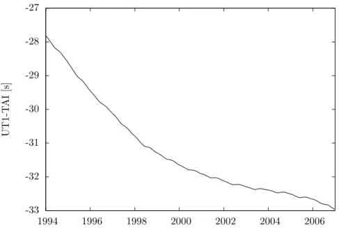
Variations of ∆UT1 consist primarily of a linear trend. This can be seen in Fig. 3.3 where a VLBI-derived

∆UT1 time series from 1994 to 2007 is displayed. Likewise, variations of length-of-day (LOD), which is the negative time derivative of ∆UT1

LOD = − ∂∆U T 1

∂t (3.17)

also show a linear trend of +1.8 ms/cy ( Morrison and Stephenson 2001 ). Besides this, LOD consists of decadal variations (e.g., Gross 2001 ), seasonal variations (e.g., Gross et al. 2004 ) and tidal variations (e.g., Yoder et al. 1981 ).

In case of an axis-symmetric Earth, tidal LOD and ∆UT1 excitations can only be generated by long-period tides, i.e., second-degree zonal components of the spherical harmonics. Nevertheless, the sources of sub-daily LOD and ∆UT1 variations are primarily of tidal nature. Tesseral and sectorial spherical harmonics are present due to asymmetries which lead to diurnal and semi-diurnal tidal forcings and, thus, to LOD and

∆UT1 variations at these periods as well (Chao et al. 1996 ). These asymmetries of the geophysical fluids are, e.g., irregular coastlines, tidal variations in bays and the non-equilibrium behavior of the oceans (e.g.

Brosche and Schuh 1998 ). The tidally forced variations can be expressed by poly-harmonic functions (e.g., Gipson 1996 , Rothacher et al. 2001 , Petit and Luzum 2010 )

d∆U T 1 =

n

X

i=1

u

cos ϕ

+ u

sin ϕ

(3.18a)

dLOD =

n

X

i=1

l

cos ϕ

+ l

sin ϕ

=

n

X

i=1

ω

(u

cos ϕ

+ u

sin ϕ

) (3.18b)

where n is the number of considered tides, ω

:=

the circular frequency of a tide and each tide ϕ

is the sum of integers (a

to f

) multiplied with the so-called fundamental arguments (or Delauney variables) and GMST (usually denoted by θ)

ϕ

= a

· ` + b

· `

+ c

· F + d

· Ω + f

· D + (θ + π) (3.19) The fundamental arguments `, `

, F, D, Ω represent the mean anomaly of the Moon and the Sun, the argument of latitude of the Moon, the elongation of the Moon from the Sun and the longitude of the ascending lunar node, respectively (e.g., Petit and Luzum 2010 ). The resulting amplitudes for the sine- and cosine-component of the tidally forced ∆UT1 and LOD variations are given by u

and u

as well as l

and l

in Eq. (3.18).

The dominating part of the sub-daily variations is due to the ocean tides where 90% of the measured tidal

∆UT1 variations are explained by a tidal ERP model based on a theoretical ocean tidal model (Chao

et al. 1996 ). Such sub-daily tidal variations based on ocean tide models were first predicted by Yoder

et al. (1981 ). Afterwards, similar predictions were made by several authors. Following Gross (2007 ), these

investigations can be divided into two groups, those before and those after the inclusion of sea surface height

altimeter observations from TOPEX/POSEIDON (Fu et al. 1994 ) which changed the ocean tidal models

significantly. Prior to TOPEX/POSEIDON, e.g., Brosche (1982 ), Baader et al. (1983 ), Brosche et al.

18 3. Theory of Sub-daily Earth Rotation

-33 -32 -31 -30 -29 -28 -27

1994 1996 1998 2000 2002 2004 2006

U T 1 -T A I [s ]

Figure 3.3: 13 year long ∆UT1 time series determined from a VLBI solution.

(1989 ), Seiler (1990 ), Seiler (1991 ), Wünsch and Busshoff (1992 ), Dickman (1993 ), Gross (1993 ) and Seiler and Wünsch (1995 ) used ocean tidal models to determine a model for tidal LOD or ∆UT1 variations. Based on assimilation models, predictions were made by, e.g., Ray et al. (1994 ), Egbert et al.

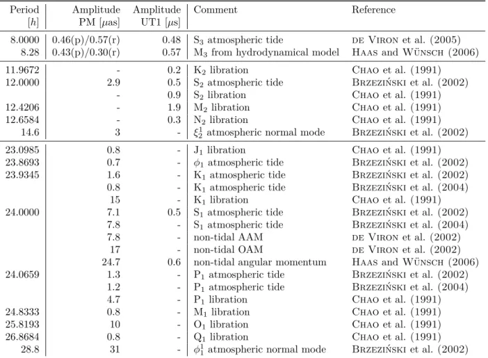
(1994 ), Chao et al. (1995 ), Chao et al. (1996 ) and Chao and Ray (1997 ). These assimilation ocean tidal models use both, an ocean tidal model and sea-surface heights measured by TOPEX/POSEIDON. In the IERS Conventions 2010 the coefficients for diurnal and semi-diurnal variations in LOD and ∆UT1 of an updated version of the Ray et al. (1994 ) model are listed in Tab. 8.3 of Petit and Luzum (2010 ).

Small variations in LOD and ∆UT1, that cannot be explained by tidal ERP models based on the theoretical ocean tidal models were detected by, e.g., Schuh and Schmitz-Hübsch (2000 ), Haas and Wünsch (2006 ) and Artz et al. (2010 ). These differences might be forced by diurnal and semi-diurnal atmospheric effects as this influence is up to two orders of magnitude below the oceanic impact (Brzeziński et al. 2002 ). These atmospheric effects are produced by gravitational forces and by non-tidal thermal forces. However, in the atmosphere, the thermal effects are expected to be much larger than the gravitational tides (e.g, Chapman and Lindzen 1970 ). These thermal effects are excited by the heating of the Sun with a basic frequency of one cycle per solar day, for which additional harmonics with integer cycles per solar day are present.

However, only the waves with diurnal, semi-diurnal and ter-diurnal periods are considered as being significant (Volland 1997 ). Furthermore, non-tidal oceanic effects might be present. This non-tidal oceanic variability is not directly related to the gravitational forcing, but generated by corresponding atmospheric tides, thus, they are called radiational ocean tides (Brzeziński et al. 2004 ). The impact of the atmosphere on the Earth’s rotation on time scales of one day and below was performed by, e.g., Zharov and Gambis (1996 ), Brzeziński et al. (2002 ), de Viron et al. (2005 ) and Brzeziński (2008 ). Concerning these predictions, several problems arise as they are usually based on AAM series which have a temporal resolution of six hours.

Certain pairs of tidal waves are mixed together and the sampling of six hours is not sufficient to resolve them (Brzeziński et al. 2002 ). Thus, it is difficult to investigate the semi-diurnal band. Nevertheless, even ter- diurnal tidal impacts were investigated by de Viron et al. (2005 ) and Haas and Wünsch (2006 ) on a model basis.

Finally, the tri-axial shape of the Earth has to be considered, as the direct effect of external torques on the

non-axis-symmetric part of the Earth leads to variations in the Earth’s rotation called libration. This effect

was investigated by, e.g., Chao et al. (1991 ), Wünsch (1991 ), Chao et al. (1996 ) as well as by Brzeziński

and Capitaine (2003 ) and Brzeziński and Capitaine (2010 ). The most recent IERS Conventions 2010

provide such a model in Tab. 5.1b of Petit and Luzum (2010 ).

3.2. Excitation of the Earth Rotation Parameters 19

3.2.2 Polar Motion

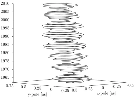
Comparable to the excitations of the Earth’s rotation rate, PM changes also exist due to various phenomena.

Besides the above mentioned free wobble, several other internal forces change the position of the CIP w.r.t. the z-axis of the TRF. Again, mass redistributions, tidal variations and angular momentum exchanges between the solid Earth and geophysical fluids are the driving forces. Figure 3.4 shows the official IERS 05C04 PM time series (Bizouard and Gambis 2009 ). The most obvious characteristic is a beat with a period of about 6.3 years. This is a superimposition of the free wobble and an almost yearly signal. The period of the free wobble has been determined by, e.g., Wilson and Haubrich (1976 ) to be 433 days and its varying amplitude is around 100 – 200 mas (3 – 6 m at the Earth’s surface; e.g., Schuh et al. 2000 ). The difference to the period of 305 days (Euler 1765 ) for a solid Earth depends on the internal structure and rheology of the Earth, e.g., the elasticity of the Earth, atmospheric, oceanic, and hydrological processes as well as the presence of a fluid core can be considered as causes. However, the relative contribution of each component is still unclear. In contrast, the yearly signal is a forced motion with a nearly constant amplitude of 100 mas (Rummel et al. 2009 ). The exciting processes are various geophysical and gravitational sources with an annual characteristic, where the largest impact is a high atmospheric pressure system over Siberia every winter (e.g., Gross et al. 2003 ). In addition, smaller variations can be detected at decadal time scales with amplitudes around 30 mas (Markowitz wobble, Gross 2007 ) and smaller variations on all measurable time scales are present. The variations with periods of one day and below, which are investigated within this thesis, belong to the latter group. They are treated in more detail below. Finally, a linear trend is present with a rate of 3.3 mas/year with a direction towards 76

longitude (e.g., Schuh et al. 2001 ).

Concerning diurnal and sub-diurnal time scales, tidal variations have the biggest impact. For an axis- symmetric Earth, no PM variations are expected due to the second-degree zonal tides but asymmetries are present in the geophysical fluids as already described in Ch. 3.2.1. Due to these asymmetries, long term PM are forced by the exchange of non-axial oceanic tidal angular momentum with the solid Earth. Fur- thermore, diurnal and semi-diurnal ERP variations are caused by tesseral and sectorial components of the spherical harmonic expansion of the tide generating potential. The tidally induced PM variations can be modeled by a poly-harmonic representation as well (e.g., Gipson 1996 )

dx

(t) =

n

X

j=1

−p

cos ψ

+ p

sin ψ

(3.20a)

dy

(t) =

n

X

j=1

p

sin ψ

+ p

cos ψ

(3.20b)

with the sine- and cosine-amplitudes of the tidal PM variations p

and p

. All other symbols correspond to Eq. (3.18). To account for retrograde PM, the individual tides ψ

are derived by inserting the integer factors of the fundamental arguments with opposite sign in Eq. (3.19). However, this is only done for the semi-diurnal tides, as the retrograde diurnal PM components are defined as nutation (see Fig. 3.1). Chao et al. (1996 ) showed that 60% of the sub-daily PM variations can be explained by the impact of diurnal and semi-diurnal ocean tides. Remaining differences can be attributed to non-tidal atmospheric and oceanic effects. It should be mentioned, that the solid Earth tides are primarily absorbed by introducing them as station position corrections to the observables as described in Ch. 4.1.

As with ∆UT1, Yoder et al. (1981 ) first discussed the effect of diurnal and semi-diurnal ocean tides on PM. Subsequently, models for sub-daily PM variations were derived from theoretical ocean tide models by, e.g., Seiler (1990 ), Seiler (1991 ), Dickman (1993 ), Gross (1993 ), Brosche and Wuensch (1994 ) and Seiler and Wünsch (1995 ). With the advent of TOPEX/POSEIDON and the integration of its sea surface height observations into ocean tide models, enhanced tidal PM models were calculated by Chao et al. (1996 ) and Chao and Ray (1997 ). In Tab 8.2 of the current IERS Conventions 2010 a model based on an ocean tide model is given where altimeter observations were assimilated.

Comparable to ∆UT1, discrepancies of these theoretical ERP models to measurements of sub-daily PM exist

(e.g., Schuh and Schmitz-Hübsch 2000 , Haas and Wünsch 2006 , Nastula et al. 2007 and Artz et al.

20 3. Theory of Sub-daily Earth Rotation

-0.25 -0.5 0.25 0

0.5 0.75 0.5 0.25 0 -0.25 1965

1970 1975 1980 1985 1990 1995 2000 2005 2010

x-pole [as]

y-pole [as]

Figure 3.4: Pole spiral from the IERS 05C04 time series ranging from 1962 to 2010.

2010 ). The reason for these differences can again be attributed to missing non-tidal oceanic or atmospheric effects in the ERP models that are based on theoretical ocean tide models. Atmospheric excitations have been investigated by Zharov and Gambis (1996 ), Brzeziński et al. (2002 ) and de Viron et al. (2005 ).

In addition, Brzeziński et al. (2004 ) and Brzeziński (2008 ) determined the impact of non-tidal oceanic angular momentum due to radiational atmospheric tides as well as the impact of the atmospheric tides themselves. de Viron et al. (2002 ) predicted diurnal PM variations based on non-tidal AAM and OAM and Haas and Wünsch (2006 ) reported diurnal PM excitation based on a non-tidal angular momentum approach. Concerning the semi-diurnal predictions based on AAM time series, these are uncertain as the pro- and retrograde PM components cannot be separated due to the six hour long temporal resolution of the AAM time series (Brzeziński et al. 2004 ). AAM series with a better resolution are currently only available for limited time spans, e.g., Salstein et al. (2008 ) derived hourly wind-based excitations for polar motion of the CONT02 and CONT05 periods.

Similar to ∆UT1, the effects of the tri-axial shape of the Earth are present in PM although not that

pronounced. This effect was investigated by Chao et al. (1991 ) and Chao et al. (1996 ). To account for

libration in the diurnal prograde PM band, the IERS Conventions 2010 provides the amplitudes for 10 tidal

constituents in Tab. 5.1a of Petit and Luzum (2010 ).

21

4. Measuring Earth Rotation Parameters with VLBI

VLBI is a space geodetic technique based on radio interferometry. The interferometer is built up of two locally separated antennas with a maximum distance of about 10,000 km. These antennas observe a radio signal of currently 2.3 and 8.4 GHz that is emitted by extragalactic radio sources such as quasars or radio galaxies. A detailed description of the VLBI space segment is given by, e.g, Heinkelmann (2008 ). The observed radio signal is recorded digitally at each antenna together with a highly precise time information provided by a hydrogen maser. The signals are then sent to a correlation center to be cross-correlated. In this way, the primary observables for the VLBI analysis, the delay and the delay rate, are generated (e.g., Whitney 2000 ).

Within the IVS, a global network of about 40 VLBI stations currently exists. In a standard VLBI observing session of 24 hours duration, three to 15 of them observe in general 15 to 60 radio sources while in specific observing sessions, up to 260 radio sources are observed. The VLBI sessions, of which on average three are performed per week, are used to estimate various parameters such as the EOPs. In addition, special single baseline VLBI sessions, so-called Intensives, of one hour duration are observed almost daily to provide continuous ∆UT1 estimates (e.g., Robertson et al. 1985 , Luzum and Nothnagel 2010 ).

In this section, the basic principle of VLBI as well as the process of parameter estimation are briefly described.

Furthermore, the specifics for the determination of ERPs are presented with an emphasis on the determination of sub-daily ERP representations.

4.1 The Basic Principle of VLBI

The general configuration of VLBI consists of two antennas, building a baseline b, which simultaneously observe the incoming electromagnetic wave front which is emitted by the same radio source and which travels along the unit vector k. This basic principle is depicted in Fig. 4.1. Although the radio signal is initially a sphere, a planar wave front can be assumed without any loss of generality, as the radio sources are very distant (2 to 12 billion light-years). Today, the primary VLBI observable is the time delay τ, i.e., the time difference between the reception of the radio signal at antenna one and antenna two. Prior to the recording of the signal at the antennas, it traveled through the interstellar space, the Solar System as well as the Earth’s atmosphere. On this path, it is affected by various electromagnetic and gravitational impact factors. Furthermore, the geometry is changing between the reception of the signal at antenna one and two, e.g., due to the Earth’s rotation. All of these factors have to be considered during a VLBI analysis. Within this thesis, only the major points are mentioned, a more detailed description of general principles of VLBI can be found in many publications, e.g., Thomas (1972 ), Campbell (1987 ), Sovers et al. (1998 ) or Takahashi et al. (2000 ).

During a standard VLBI session, several radio telescopes observe several sources over a longer time span, nevertheless, the basic principle as shown in Fig. 4.1 is sufficient to describe the principle of VLBI. This holds especially, as the correlator generates the observables independently for each baseline (Sovers et al.

1998 ). The geometric time delay τ

is the difference in arrival time of the radio signal between two observing telescopes, where an ideal instrumentation, synchronization and a vacuum between the source and the tele- scopes is assumed. As a planar wave front is assumed, the geometric delay can be computed in a right-angled triangle (e.g., Takahashi et al. 2000 )

τ

= t

− t

= − 1

c b · k (4.1)

with the VLBI vector baseline b = r

− r

computed from the position vectors of two VLBI telescopes r

and

the unit vector in the direction of the radio source k. t

and t

are the arrival times at the two telescopes

22 4. Measuring Earth Rotation Parameters with VLBI

antenna 2

r2

geocenter

r1 b c·τ

k

antenna 1 planar

wa ve fron

ts

radio source spherical wave fronts

Figure 4.1: The basic principle of VLBI.

as measured on the Earth’s surface, or strictly speaking the geoid. Finally, c denotes the velocity of light.

However, this equation only holds if the baseline vector and the unit vector in source direction are given in the same reference system. Usually, the station positions are given in a TRF and the sources in a CRF. Thus, a transformation between these two frames is necessary. As demonstrated in Ch. 3.1, this can be realized via Eq. (3.7) by using the EOPs.

To achieve the entire accuracy of VLBI, the geometric time delay has to be expressed in a quasi-inertial barycentric system. Thus, several transformations are necessary. A detailed description of these steps can be found, e.g., in Schuh (1987 ), Sovers et al. (1998 ) or Takahashi et al. (2000 ). The principle procedure is to account for the time-dependence of the baseline length ∆b at the epoch t

, where the signal has been recorded at station one, e.g., due to Earth tides or tectonic motions. Subsequently, the baseline is transformed from the geocentric TRF to the geocentric CRF

B

(t

) = Q(t

) · R(t

) · W(t

) · (b + ∆b(t

)) (4.2)

After applying a Lorentz transformation of B

(t

), the baseline B

(T

) is given in a frame at rest relative to the center of mass of the Solar system (Solar System Barycentric (SSB) frame) which is rotationally aligned to the geocentric CRF. This transformation is applied to account for relativistic effects that arise due to the motion of the observing sites w.r.t. the barycenter. The epoch T

is now representing the time where the radio signal is received at antenna one, although measured in the barycentric system. In this SSB frame, the geometric delay is calculated (e.g., Sovers et al. 1998 )

T

= − 1 c

k · B

(T

)

1 − k · v

(4.3)

where v

is the velocity of antenna two in the SSB frame and the source unit vector in the CRF is given by k =





− cos α · cos δ sin α · cos δ

sin δ



 (4.4)

with the source coordinates in right ascension α and declination β. This delay is corrected for the relativistic

changes caused by the gravitational fields of the Sun, the Planets and the Earth. Finally, another Lorentz