Polar Science

(1)

Vp/Vs-ratios and anisotropy on the northern Jan Mayen Ridge, North Atlantic, determined from ocean bottom seismic data

Aleksandre Kandilarov

^a

, Rolf Mjelde

^a^,^*

, Ernst Flueh

^b

, Rolf Birger Pedersen

^a

aDepartment of Earth Science, University of Bergen, Allegaten 41, 5007, Bergen, Norway

bGEOMAR, Kiel, Germany

a r t i c l e i n f o

Article history:

Received 16 March 2015 Received in revised form 17 June 2015

Accepted 29 June 2015 Available online 4 July 2015

Keywords:

Vp/Vs-ratio Seismic anisotropy Jan Mayen Ridge Continental rifting Icelandic crust Oceanic spreading Ocean bottom seismometers

a b s t r a c t

In order to gain insight into the lithology and crustal evolution of the northern Jan Mayen Ridge, North Atlantic, the horizontal components of an Ocean Bottom Seismometer (OBS) dataset were analyzed with regard to Vp/Vs-modeling and seismic anisotropy. The modeling suggests that the northernmost part of the ridge consists of Icelandic type oceanic crust, bordered to the north by anomalously thick oceanic crust formed at the Mohns spreading ridge. The modeled Vp/Vs-ratios suggest variations in gabbroic composition and present-day temperatures in the area. Anisotropy analysis reveals a fast S-wave component along the Jan Mayen Ridge. This pattern of anisotropy is most readily interpreted as dikes intruded along the ridge, suggesting that the magmatism can be related to the development of a leaky transform since Early Oligocene.

1. Introduction

It is well established that the Jan Mayen Ridge, North Atlantic, at least partly represents a continental sliver rifted off East Greenland (e.g.Myhre et al., 1984; Gudlaugsson et al., 1988,Fig. 1). The western and eastern boundaries of the ridge have been described byKodaira et al. (1997); Mjelde et al. (2008a)andBreivik et al. (2012). In 2006, an Ocean Bottom Seismic (OBS) survey was conducted along the northernmost part of the ridge, mainly aiming at identifying the northern termination of the continental ridge (Kandilarov et al., 2012, Fig. 2). By modeling the OBS vertical components, com- bined with gravity modeling,Kandilarov et al. (2012)divided the northernmost part of the ridge into three segments from south to north; continental crust, Icelandic type oceanic crust, and oceanic crust accreted within the Mohns Ridge system.

Modeling of OBS horizontal components have earlier success- fully constrained crustal lithology further south on the ridge (Mjelde et al., 2007). The main aim with the present study is thus to obtain Vp/Vs-ratios from the modeling of the OBS horizontal

component data acquired in 2006, building on the P-wave and density models described byKandilarov et al. (2012), in order to test the hypothesis outlining the northernmost part of the ridge as an oceanic plateau. Furthermore, the horizontal components will be explored with regard to seismic anisotropy, which could provide insight into tectono-magmatic dynamics (e.g. Mjelde et al., 2003).

2. Tectonic setting

The continental rifting following the collapse of the Caledonian mountain range occurred during several rift episodes over a time span of about 350 myr, culminating with continental break-up between Norway and Greenland in the early Eocene (magnetic anomaly 24r, ~53 Ma, e.g.Talwani and Eldholm, 1977; Cande and Kent, 1995). Oceanic spreading lasted around 20 myr (until ~33 Ma, magnetic anomaly 13a) at the Reykjanes, Aegir and Mohns Ridges (Fig. 1). During this phase, spreading along the northern Mid-Atlantic Ridge was simultaneous with spreading in the Lab- rador sea (Talwani and Eldholm, 1977; Tessensohn and Piepjohn, 2000). Voluminous magmatic activity accompanied the separation of Norway and Greenland, leading to the formation of thicker oceanic crust. Thick igneous layers were also intruded as sills into

*Corresponding author.

E-mail address:Rolf.Mjelde@geo.uib.no(R. Mjelde).

Contents lists available atScienceDirect

Polar Science

j o u rn a l h o m e p a g e : h t t p : // e e s. e ls e v ie r. co m / p o l a r/

http://dx.doi.org/10.1016/j.polar.2015.06.001

Polar Science 9 (2015) 293e310

(2)

the continental crust or extruded sub-aerially asﬂood basalts. This magmatism decreased signiﬁcantly after 5e10 myrs of oceanic spreading (Eldholm et al., 1989; White and McKenzie, 1989; Mjelde et al., 2008a).

The second stage of the northern North Atlantic evolution started in the early Oligocene (~33 Ma) when the spreading in the Labrador Sea ceased and Greenland became attached to the North American plate (Torsvik et al., 2001). This was accompanied by a change in the relative plate motion between the European and North American plates from NNWdSSE to NWeSE. Spreading along the Aegir Ridge decreased gradually and the ridge became extinct at ~25 Ma (magnetic anomaly 6e7,Talwani and Eldholm, 1977; Tessensohn and Piepjohn, 2000; Mosar et al., 2002). The spreading along the Aegir Ridge was accompanied by simultaneous continental rifting on East Greenland from about 43.5 Ma until the Kolbeinsey spreading rift initiated at around 24 Ma (Mjelde et al., 2008a). Initially, the spreading along the northern Kolbeinsey Ridge was relatively slow and subject to modest volcanic activity.

About 3 myr after the break-up the magmatic activity increased due to the inﬂuence of the Icelandic hot-spot, and thicker than normal oceanic crust has been generated since (Kodaira et al., 1997; Mjelde et al., 2007, 2008a).

The eastern side of the Jan Mayen micro-continent conjugate to the Møre segment on the Norwegian margin is a volcanic margin, while the western side of the micro-continent represents a non- volcanic margin (Gudlaugsson et al., 1988; Kodaira et al., 1998;

Mjelde et al., 2007, 2008a; Breivik et al., 2012).

3. The P-wave models

Since the Vp/Vs-modeling presented in this paper is based on the P-wave models ofKandilarov et al. (2012), we will here sum- marize theirfindings, which divides the northern Jan Mayen Ridge into a southern continental segment, a middle segment with Ice- landic affinities and a northern oceanic segment influenced by the Mohns Ridge (Figs. 3 and 4).

Continental crust, characterized by relatively low crustal P-wave velocities (5.75e6.85 km/h), is inferred along the southern parts of the two lines south of the Continent Ocean Boundary (COB), located near OBS 10 along Line 1 and near the mid-point between OBS 32 and 33 on Line 2. The COB is interpreted in the center of an about 20 km wide Continent Ocean Transition (COT). The continental crust is overlain by three pre-opening sedimentary sequences dated as pre-Cretaceous, Cretaceous, Paleocene/Early Eocene, respectively (Gudlaugsson et al., 1988). Two younger sequences of post-rifting Cenozoic sediments were deposited on top of the older sequences.

Oceanic crust related to accretion at the Mohns Ridge, consisting of layers 2, 3A and 3B, is present north of OBS 16 on Line 1 and OBS 28 on Line 2. The oceanic crust is characterized by anomalously large thickness and high P-wave velocities in layer 3B, which is indicative of elevated mantle temperatures. Thisﬁnding explains the anomalously shallow bathymetry of the area. The oceanic accreted crust is overlain by a thin layer of Late Cenozoic marine sediments.

Fig. 1.Map of the North Atlantic showing the two studied proﬁles (red lines) and the main topographic and bathymetric features: RReReykjanes Ridge, GIReGreenlandeIceland Ridge, FIReFaeroe-Iceland Ridge, FIeFaeroe Islands, SIeShetland Islands, MMeMøre Margin, MMHeMøre Marginal High, AReAegir Ridge, JMReJan Mayen Ridge, JMBeJan Mayen Basin, KbReKolbeinsey Ridge, EGMeEast Greenland Margin, WJMFZeWest Jan Mayen Fracture Zone, EJMFZeEast Jan Mayen Fracture Zone, VMeVøring Margin, LMe Lofoten Margin, MoReMohn Ridge, KnReKnipovich Ridge. (For interpretation of the references to colour in thisﬁgure legend, the reader is referred to the web version of this article.)

(3)

The segment between the COB and the Mohns Ridge oceanic crust is interpreted as an Icelandic type oceanic plateau (anomalously thick oceanic crust), based on the similarities with Iceland in crustal layering and P-wave velocities (Bjarnason et al., 1993;

Allen et al., 2002; Gudmundsson, 2003; Sigmundsson, 2006).

Sampling of 32e24 Ma lavas, gabbros and volcano-clastic sediments along the southern slope of the West Jan Mayen Fracture Zone (WJMFZ) has conﬁrmed that the northernmost Jan Mayen Ridge formed within an area of Oligocene magmatism (Pedersen et al., 2010). Gernigon et al. (2009)and Kandilarov et al. (2012) attribute the anomalous magmatism to a discrete leaky transform developing along the Jan Mayen Fracture Zone, following the 33 Ma change in plate motions. Note that the COB follows the trend of the East Jan Mayen Fracture Zone (EJMFZ), supporting this interpretation.

It is unlikely that thefloating reflectors included in the lower crust and upper mantle in the model for Line 1 (Fig. 3) represent remnants of subduction, since it is well documented on the conjugate Norwegian Margin that Caledonian collisional features have been removed by later extension (Mjelde et al., 2012). Such floating reflectors are generally interpreted in terms of shear zones or remnants of the magma plumbing system (Mjelde et al., 2009).

4. S-wave OBS data acquisition and processing

The geophysical survey performed in 2006 along the northernmost Jan Mayen Ridge collected OBS data, multichannel seismic data (MCS) and gravity data simultaneously (Kandilarov et al., 2012). Data were acquired along two ~220 km and 165 km long lines, striking NS and NEeSW, respectively.Fig. 2shows the location of the survey lines, as well as previous OBS surveys in the area (Kodaira et al., 1998; Mjelde et al., 2007, 2008b). The seismic source employed in 2006 consisted of a tuned array of seven air-guns with a total volume of 40 L, which was shot every 100 m at a depth of about 10 m. The source can be considered as a point source generating P-waves only. Encountering an impedance contrast, i.e.

the seaﬂoor, parts of the energy will be converted to S-waves. In an isotropic model with horizontal layers all converted S-waves will be SV waves, but in an anisotropic subsurface the S-waves will split into several waves propagating according to the speciﬁc anisotropic symmetry (Crampin, 1990).

A total of 15 OBSs and 20 OBHs (Ocean Bottom Hydrophone) stations were deployed along the two lines. The OBSs were equipped with three orthogonally mounted geophones and one hydrophone. These instruments were thus capable of recording both compressional waves (P-waves) and shear waves (S-waves).

Fig. 2.Map of the survey area showing the two seismic profiles and the locations of the instruments. Crosses denote the four-component instruments (OBS), while the dots denote the one-component instruments (OBH). Lines L3S-1995 to L6-1995 are profiles presented byKodaira et al. (1998)andMjelde et al. (2007). Line 8-00 is presented inMjelde et al. (2008b). The blue line shows the location of the northern continental-oceanic crust boundary (COB), fromKandilarov et al. (2012). The yellow line (Icelandic-Mohns boundary) shows their interpreted boundary between Icelandic type and oceanic crust related to the Mohns Ridge. JMR: Jan Mayen Ridge, EB: Eggvin Bank, WJMFZ: West Jan Mayen Fracture Zone, EJMFZ: East Jan Mayen Fracture Zone. (For interpretation of the references to colour in thisfigure legend, the reader is referred to the web version of this article.)

A. Kandilarov et al. / Polar Science 9 (2015) 293e310 295

(4)

Three instruments, 24, 26 and 29 along Line 2, did not yield useful data.

The OBS horizontal axes are randomly oriented on the sea-ﬂoor, and the vertical axis may be tilted. In order to assure reliable

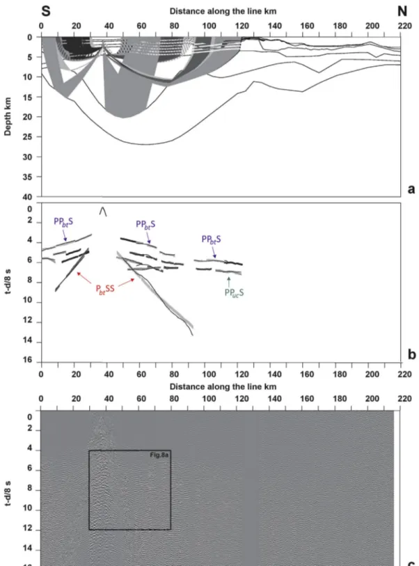
identiﬁcation of S-wave phases, the orientation of the axes of the two horizontal OBS channels ought to be known relative to the in- line (shooting) and cross-line directions, and the possible inclina- tion of the vertical axis should be estimated. Both the orientation of Fig. 3.a) P-wave velocity model of Line 1. b) Interpretation of the P-wave velocity model (Kandilarov et al., 2012).

(5)

the horizontal components and the vertical tilt can be estimated from the direct water arrival, at a certain offset range, since this wave is polarized linearly in the in-line plane. The horizontal components can subsequently be re-oriented into in-line and

cross-line components with an uncertainty of about 5 (Mjelde et al., 2002a).

The processing of the OBS data included 8 km/s velocity reduction, band-passﬁltering between 2-4 and 4e16 Hz, spiking Fig. 4.a) P-wave velocity model of Line 2. b) Interpretation of the P-wave velocity model (Kandilarov et al., 2012).

(6)

deconvolution and automatic gain control (AGC) with a window length of 0.7 s. This processing scheme was applied to all components, and is similar to the processing performed in earlier studies (Kodaira et al., 1998; Mjelde et al., 2007; Breivik et al., 2012). In the near-offset range we also used the unﬁltered data during the interpretation, sinceﬁltering caused strong ringing of the high- amplitude direct water arrival. The reader is referred to Mjelde et al. (2002a)for more details on processing of multi-component OBS data. Some examples of processed OBS data are shown in Figs. 5e7, and blow-ups of parts of the data are presented inFig. 8.

5. Vp/Vs-modeling: background and procedure 5.1. Vp/Vs-ratio versus lithology

One of the limitations of P-wave models arises from the fact that different lithologies - for instance sand and shaleegenerally have similar P-wave velocities (e.g.Christensen, 1996). Laboratory experiments and case studies have shown that knowing both the P- and S-wave velocities can help constrain the lithology.Domenico (1984) found the following Vp/Vs-ratios for consolidated sedimentary rocks; sandstones: 1.59e1.76, limestone: 1.84e1.99, shales: 1.70e3.00.

High sedimentary Vp/Vs-ratios (>3.00) are attributed to low degrees of compaction and are typical for shallow marine sediments (Bromirski et al., 1990; Chung et al., 1990; Mjelde et al., 2007). Increasing the lithostatic pressure in sedimentary rocks re- duces their porosity, resulting in a decrease in the Vp/Vs-ratio (e.g.

Chung et al., 1990).

The Vp/Vs-ratio is particularly sensitive to the content of quartz, and the Vp/Vs-ratio thus offers a means to distinguish between felsic and maﬁc crystalline basement compositions.Holbrook et al.

(1992) reviewed Vp/Vs-ratios for different crystalline rocks, and reported values that varied from 1.71 in granite (felsic) and 1.78 in granodiorite, to 1.84 in gabbro (maﬁc).

5.2. S-wave mode conversions

Compressional P-waves are generated when air-guns areﬁred in the water. As the P-waves encounter boundaries between layers with different acoustic impedance, parts of the energy will reﬂect or refract (depending on the angle-of-incidence) as both P- and S- waves (e.gDigranes et al., 1996).

The observed shear wave phases are usually divided into three typesewaves traveling with apparent P-wave velocity converted on the way up (PPS arrivals), waves converted on the way down and thusly traveling with apparent S-wave velocity (PSS arrivals) and waves converted at the reflecting/critically refracting boundary (target converted arrivals; Mjelde et al., 2002a). PPS arrivals are easily identified on horizontal component seismograms, since they appear as delayed versions of the P-wave arrivals observed on the hydrophone or vertical geophone seismograms. The time delay reflects their proportion of the ray-path as slower S-waves. PSS arrivals have a characteristic slope corresponding to a seismic velocity of 4e5 km/s, which generally reflects the range of typical crustal S-wave velocities.

5.3. S-wave modeling

The P-wave velocity models (Figs. 3a and 4a) ofKandilarov et al.

(2012), consisting of seven layers, were used as basis for the S-wave modeling. These P-wave models were obtained by using the 2-D ray-tracing software Rayinvr (Zelt and Ellis, 1988; Zelt and Smith, 1992). This software allows the tracing of reﬂected-, refracted- and head waves in the different model layers, the calculation of

their travel-times and comparison with travel-times interpreted from the OBS seismograms. By assigning Poisson's ratios to the layers of a P-wave velocity model, Rayinvr may be used to simulate mode converted rays. An important assumption is that P-to-S conversions will occur at the same interfaces as those found during the P-wave modeling. By comparing theoretical travel-times with observed arrivals from the in-line component OBS seismograms we obtain a model of the Poisson's ratio, which can readily be converted into a Vp/Vs-ratio model (Figs. 5e7;Stein and Wysession, 2003). The modeling thus consists of estimating the conversion boundary for each interpreted arrival, and the Vp/Vs-ratio within each layer. We modeled the data from each instrument separately and derived the Vp/Vs ratio in each layer by a layer stripping approach (Zelt, 1999; Zelt et al., 2003). A variation in Vp/Vs-ratio within each layer was achieved by merging the models from all instruments (Figs. 9 and 10). The resolution of the obtained traveltime model is not high enough to allow amplitude modeling, including calculation of synthetic seismograms, to be performed (Mjelde et al., 2002a).

5.4. Uncertainty estimates

The ﬁt between the calculated and observed travel times is estimated byc²given by the formula:

c²¼1 n

Xⁿ

i¼1

t_0it_ci U_i

₂

wherenis the number of data points,t0iis the observed andtciis the calculated travel-time of the i-th data point andU_iis the traveltime picking uncertainty of the i-th data point. Ac²value around one means an optimalfit between the observed and calculated travel-times for the given uncertainty. However, 3-D wave propa- gation effects (out-of plane ray paths), unresolvable small scale structures and structural inhomogeneities (Zelt et al., 2003) will prohibit an ideal fit. Therefore, additional indicators must be considered when estimating the reliability of thefinal model. Such quality indicators are the signal-to-noise ratio for individual phases and the ray-coverage for different parts of the model (Breivik et al., 2005; Mjelde et al., 2005). The reliability of the Vp/Vs-model will thus depend on the validity of the underlying P-wave velocity model, the data quality of the horizontal components and the uncertainty of the travel-time picks.

We used linearly variable travel time picking uncertainty, which was set to 75 ms for the arrivals closest to the instrument and 120 ms for arrivals at maximum offset (200 km). An uncertainty up to 120 ms was also used for unclear arrivals. During the modeling we attempted to use all coherent arrivals and minimize theirc² values. Thec²values and the number of rays sampling each model layer are given inTable 1.

The amount of modeled data may also be shown as the variation of the ray density within the model. This allows assessment of the spatial resolution of the model. We quantiﬁed the ray density by computing and presenting illumination diagrams (Fig. 11). The diagrams were obtained by dividing the models into rectangular 102.5 km cells and computing the number of ray-hits in each cell relative to all ray-hits, expressed as a percentage. If our models were illuminated uniformly, each cell of Line 1 would contain 0.28%

of the total ray-hits. For Line 2, the corresponding number would 0.37%. These values were used as criteria to distinguish between well and poorly illuminated model cells. Cells having more than 0.28% of ray-hits for Line 1 and 0.37% for Line 2 are considered well resolved. Cells having fewer ray-hits are less well resolved, while cells with no ray-hits are unresolved (shown as black areas in

(7)

Fig. 11). The illumination diagrams show that the shallow-to- middle depth parts of both models are well resolved, and that the resolution is decreasing to zero at the bottom and towards the ends of the models. The error in the modeled Vp/Vs-ratios is estimated to be±0.03 within the white areas of Fig. 11,±0.05 in the orange/

yellow cells (in web version) and ±0.07 in the red cells. Black shading indicates unresolved model. These uncertainties are in

agreement with those estimated by Mjelde et al. (2007)further southwards on the ridge.

5.5. Particle motion analysis

When a shear wave enters an anisotropic medium it will split into two (or more) different waves polarized along and Fig. 5.a) Mode converted rays traced for OBS 05, Line 1. The solid lines show the portions of the ray-paths where the rays travel as P-waves, whereas the dashed ray-paths represent the S-waves. b) Calculated (thin solid lines) versus observed (gray shaded bars) travel time curves for the rays traced. The width of the bars reﬂects the picking uncertainty. Most important arrivals are: PPbtS: converted on the way up at base Tertiary, PPucS: converted on the way up at the top of the upper crust, PbtSS: converted on way down at the base Tertiary. c) Seismogram from the in-line horizontal channel. The inset is blown up inFig. 8a.

(8)

perpendicular to the structures causing the anisotropy (Crampin, 1990; Mjelde et al., 2002a,b,c; Stein and Wysession, 2003).

Crampin (1990) discusses ﬁve possible reasons for anisotropy in the crust: 1) oriented crystals (crystalline anisotropy); 2) aligned fabric, such as aligned grains (lithological anisotropy); 3) regular sequences of isotropic bodies such as periodic thin layers or dikes (long wave-length anisotropy); 4) direct stress-induced

anisotropy; 5) aligned micro-fractures (extensive-dilatancy anisotropy, EDA). According toCrampin (1990), shear wave split- ting is primarily caused by aligned crustal cracks/fractures. A shear wave polarized along the cracks will travel faster than a wave polarized perpendicular to the cracks. Accordingly, the two types of polarized shear waves deﬁne the“fast” and“slow” directions of anisotropy.

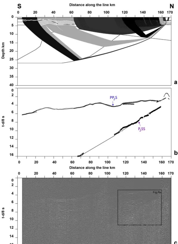
Fig. 6.a) Mode converted rays traced for OBS 21, Line 2. The solid lines show the portions of the ray-paths where the rays travel as P-waves, whereas the dashed ray-paths represent the S-waves. b) Calculated (thin solid lines) versus observed (gray shaded bars) travel time curves for the rays traced. The width of the bars reﬂects the picking uncertainty. Most important arrivals are: PP2S: converted on the way up at the top of oceanic layer 2, P2SS: converted on way down at the top of oceanic layer 2. c) Seismogram from the in-line horizontal channel. The inset is blown up inFig. 8b.

(9)

Particle motion diagrams may be generated using unﬁltered S- wave amplitudes from the three mutually perpendicular geophone channels (e.g.Stein and Wysession, 2003). These are called polarization diagrams or hodograms (Crampin, 1990; Mjelde et al., 2002a,c). Possible anisotropy can be found by computing particle motion diagrams over a time window trailing the onset of an

identiﬁed S-wave. If anisotropy is present, the hodogram will show particle motions in two preferred directions, corresponding to the fast and slow directions.

Comparisons of hodogram analyses of PSS arrivals from raw and filtered OBS data showed no significant differences, except that filtered data provided smoother polarization diagrams. Examples Fig. 7.a) Mode converted rays traced for OBS 28, Line 2. The solid lines show the portions of the ray-paths where the rays travel as P-waves, whereas the dashed ray-paths represent the S-waves. b) Calculated (thin solid lines) versus observed (gray shaded bars) travel time curves for the rays traced. The width of the bars reflects the picking uncertainty. Most important arrivals are: PP2S: converted on the way up at the top of layer oceanic 2, P2SS: converted on way down at the top of oceanic layer 2, PP3AS: converted on the way up at the top of layer 3A, P3ASS: converted on way down at the top of layer 3B, PP3BS: converted on the way up at the top of layer 3B. c) Seismogram from the in-line horizontal channel. The inset is blown up inFig. 8c.

(10)

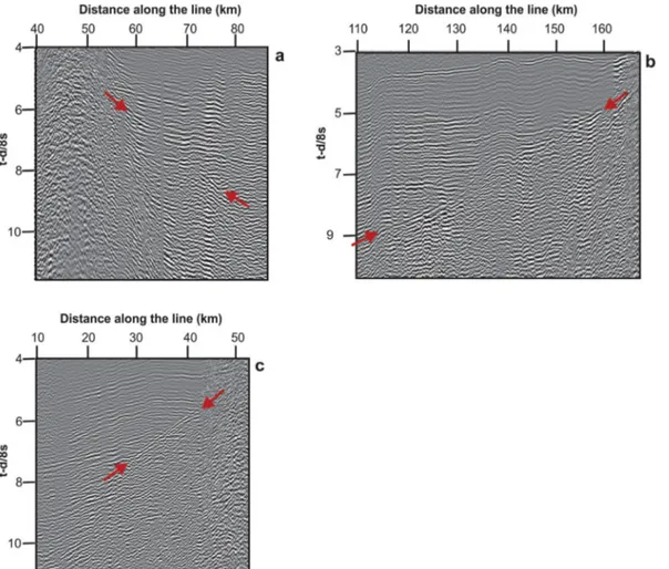
Fig. 8.Blow-up of parts of the data shown inFigs. 5e7. The red arrows point at parts of the PSS phase. (For interpretation of the references to colour in thisﬁgure legend, the reader is referred to the web version of this article.)

Fig. 9.Vp/Vs-model along Line 1 and the locations of the modeled instruments. The patterned, grey areas show the parts of the model without ray penetration.

(11)

from the hodogram analysis are shown inFigs. 12e13. We derived two sets of results; the azimuth of the fast and slow anisotropy directions and the percentage of anisotropy in the medium, ANI, which was calculated using the following formula: (Stein and Wysession, 2003)

ANI¼100vfastvslow

vaverage %;vaverage¼vfastþvslow

2 (1)

where vfastis the average shear wave velocity along the fast direction and v_slowalong the slow direction. After substituting for vaveragein Eq.(1)we obtain

ANI¼200v_fastv_slow vfastþvslow

% (2)

The average v_fast and v_slow may be expressed as vfast¼^S_t^fast_fast;vslow¼^S_t^slow_slow, and substituted in Eq.(2)we get:

ANI¼200

Sfast

tfast^S_t_slow^slow

Sfast

tfastþ^S_t^slow

slow

% (3)

Because the shear waves polarized along the fast and slow anisotropy directions will travel with different velocities, they will necessarily have different ray-paths. If the arrival times of the fast and slow phases are close, we may assume thatS_fastzS_slowand then Eq.(3)becomes

ANI¼200t_slowt_fast

t_slowþt_fast% (4)

This equation may be used to calculate the anisotropy from the onsets of the fast and slow shear wave phases interpreted from the hodogram analysis.

6. Results and discussion 6.1. Sedimentary sequences

The sequences of Oligocene and younger sediments along the two lines (model layer 1, 0e110 km along Line 1 and 0e80 km on Line 2) have high Vp/Vs-ratios, ranging from 3.2 to 8.0 along Line 1 and 4.0 to 8.0 along Line 2 (Figs. 3 and 9andFigs. 4 and 10). The Paleocene/Eocene sediments along Line 1 (model layer 2, 0e110 km) have Vp/Vs-ratios in the range 2.45e2.6, while along Line 2 (model layer 2, 0e80 km) the ratio is estimated to be 2.6e3.0.

The modeled Vp/Vs-values in the Cretaceous sediments (model layer 3, 0e90 km on Line 1 and 0e30 km on Line 2) are 2.15e2.2, while the pre-Cretaceous sediments (model layer 4, 0e90 km, Line 1 and 0e30 km, Line 2) have a Vp/Vs-value of 1.9.

The high Vp/Vs ratios in the Oligocene and younger sediments along both lines are indicative of a low degree of consolidation and Fig. 10.Vp/Vs-model along Line 2 and the locations of the modeled instruments. The patterned, grey areas show the parts of the model without ray penetration.

Table 1

Number of data points used to constrain the model parameters in each layer and the calculated RMS andc²values.

Layer No Number of data points RMS c²

Line 1

Layer 7 1404 0.141 1.756

Layer 6 4384 0.130 2.157

Layer 5 2853 0.149 1.868

Layer 4 1302 0.086 1.163

Layer 3 249 0.120 3.125

Layer 2 20 0.054 0.539

Layer 1 N/A N/A N/A

Total: 10,212 0.135 1.880

Line 2

Layer 7 3328 0.147 1.855

Layer 6 3649 0.129 1.429

Layer 5 1232 0.073 0.882

Layer 4 780 0.110 2.154

Layer 3 237 0.104 2.294

Layer 2 12 0.169 3.132

Layer 1

Total 9238 0.126 1.584

(12)

high porosity in these formations (Figs. 9 and 10). These results are in line withMjelde et al. (2007), who observed similar Vp/Vs-ratios (2.3e7.9) further south on the ridge (Fig. 2). High porosity also dominates the post-opening sediments along the conjugate Nor- wegian Margin, where the Vp/Vs-ratios are modeled at 2.0e4.5 (Mjelde et al., 2009).

In the Early Tertiary/Cretaceous sequences further south on the ridge the observed Vp/Vs-values are estimated at 1.9e2.2 (Fig. 2, Mjelde et al., 2007). Our somewhat higher values of 2.15e2.2

indicate higher shale content on the northernmost part of the ridge (Figs. 9 and 10).Mjelde et al. (2007)modeled a Vp/Vs-value of 1.9 in the pre-Cretaceous sedimentary sequences, which is in agreement with our models. The lithology of the pre-Cretaceous units is interpreted as shale dominated, with lower Vp/Vs-ratio than in the Cretaceous sequence due to increased compaction and lower porosities.

Along the conjugate Norwegian Margin the Vp/Vs-ratios in the Cretaceous sedimentary sequences are generally lower (1.75e1.95) Fig. 11.Illumination diagram of the Vp/Vs-model along Line 1 (a) and Line 2 (b). White area is best resolved, while black indicated unresolved part. See text for details.

(13)

than those found in our models (Figs. 9 and 10,Mjelde et al., 2009).

Similarly, the pre-Cretaceous sequences along the Norwegian Margin have lower Vp/Vs-ratios (1.7e1.85) compared with our models. This difference may partly be explained by the fact that the Cretaceous and pre-Cretaceous sequences along the Norwegian Margin are buried signiﬁcantly deeper (2e8 km for Cretaceous and 5e12 for pre-Cretaceous units) compared with our study area (1e2 km for Cretaceous and 1.5e5 km for pre-Cretaceous units). It is likely that these sequences were subject to smaller maximum burial depth on the (proto) Jan Mayen Ridge, and the ridge has been subject to later uplift. Both these factors imply a higher degree of porosity and increased Vp/Vs-ratio on the Jan Mayen Ridge.

Furthermore, it is likely that the modeled differences imply that the shale content in the Cretaceous and pre-Cretaceous sequences on the Jan Mayen Ridge is higher compared with the Norwegian Margin.

6.2. Oceanic crust

The Vp/Vs-ratio in oceanic layer 2 is modeled at 1.9 along Line 1 (140e220 km, model layer 4) and 1.85e2.2 along Line 2 (90e170 km, model layers 3, 4 and 5,Figs. 9 and 10). These values compares well with the values found for the area west of the Jan Mayen Ridge and on the Møre Marginal High (Mjelde et al., 2002c, 2003; 2007, 2009). The modeled variability may be explained by differences in crack quantity and porosity.

For Line 1 the modeled oceanic layer 3A Vp/Vs-value is 1.9 (model layer 5, 140e220 km), and for oceanic layer 3B (model layer 6) it is estimated at 1.85. The model of line 2 reveals no sub-division of oceanic layer 3, for which a Vp/Vs-ratio of 1.85 is estimated.

Kandilarov et al. (2012)interpreted the elevated P-wave velocities found in oceanic 3 as indicative of elevated mantle temperatures, which increases the Mg component in the melt. This interpretation Fig. 12.Results from the hodogram analysis of OBS 21, Line 2. a) Horizontal seismogram used in the Vp/Vs-modelling. The white arrow shows the location of the analyzed PSS arrival. b) Vertical (V), horizontal inline (HI) and horizontal cross-line (HC) traces of the analyzed PSS arrival. The left end of the red window marks the onset of the shear wave polarized along the fast anisotropy direction, and the width of the window is the time interval used to calculate the particle diagrams. The blue window shows the same for the shear wave polarized along the slow anisotropy direction. c) Polarization diagram of the fast shear wave calculated over the red time window shown in b). d) Polarization diagram of the slow shear wave calculated over the blue time window shown in b). e) Polarization diagram over the entire time interval from the onset of the fast wave to the end of the slow wave. (For interpretation of the references to colour in thisﬁgure legend, the reader is referred to the web version of this article.)

(14)

would imply the presence of lower than normal Vp/Vs-ratios, since increasing the Mg content at the expense of Fe will reduce the Vp/

Vs-ratio (Christensen, 1996). Such a model is valid for the area west of the Jan Mayen Ridge and on the Møre Marginal High, where Vp/

Vs-ratios of 1.80 have been inferred in oceanic layer 3 (Mjelde et al., 2002c, 2003; 2007). However, our modeled average Vp/Vs-ratio for oceanic layer 3 is 1.85, which is indicative of normal temperature gabbroic composition. The presence of some amounts of serpentinized peridotites in the lower crust would increase both the P-wave velocities and the Vp/Vs-ratio (Carson and Miller, 1997), explaining the observations in our study area.

6.3. Continental crust

The upper continental crust is well illuminated along Line 1 (model layer 5, 0e90 km,Figs. 11 and 13a), but only to about 20 km

distance southwards from the COB along Line 2 (model layer 5, 10e30 km,Figs. 10 and 11b). Along Line 1 the upper continental crust is found to have a Vp/Vs-ratio in the range 1.8e1.85, while along Line 2 we modeled a value of 1.85.

The lower continental crust along Line 2 is not illuminated (model layer 6, 0e30 km). Along Line 1 only the two extremities of this layer were illuminated (model layer 6, 0e90 km). The southern part is modeled to a Vp/Vs-value of 1.75 and the northern part expresses a value of 1.85.

The average Vp/Vs-value of 1.85 modeled in the upper (crystalline) continental crust (Figs. 9 and 10) is in accordance with the results ofKodaira et al. (1998)andMjelde et al. (2007)further south on the ridge. The same applies to the relatively low P-wave velocity modeled for the uppermost part of the crust (about 5.8 km/s;

Kandilarov et al., 2012). We are in line with the interpretation of Kodaira et al. (1998)andMjelde et al. (2007), which suggests that Fig. 13.Results from the hodogram analysis of OBS 20, Line 1. a) Horizontal seismogram used in the Vp/Vs-modeling. The white arrow shows the location of the analyzed PSS arrival. b) Vertical (V), horizontal inline (HI) and horizontal cross-line (HC) traces of the analyzed PSS arrival. The left end of the red window marks the onset of the shear wave polarized along the fast anisotropy direction, and the width of the window is the time interval used to calculate the particle diagrams. The blue window shows the same for the shear wave polarized along the slow anisotropy direction. c) Polarization diagram of the fast shear wave calculated over the red time window shown in b). d) Polarization diagram of the slow shear wave calculated over the blue time window shown in b). e) Polarization diagram over the entire time interval from the onset of the fast wave to the end of the slow wave. (For interpretation of the references to colour in thisﬁgure legend, the reader is referred to the web version of this article.)

(15)

the relatively low P-wave velocity and high Vp/Vs-ratio, down to about 10 km depth, may be explained by an intermediate rock composition and increased quantity of cracks.

Along the western side further south along the ridge,Mjelde et al. (2002c)modeled a Vp/Vs-ratio of 1.75 in the lower crust.

We observe the same value along the southernmost part of line 1, and interpret this part of the crust as consisting of intermediate/felsic rocks. Further north close to the COB, the Vp/Vs-ratio increases to 1.85, which is indicative of maﬁc rock composition.

A similar interpretation was made on the eastern side further south of the ridge, were Vp/Vs-ratios as high as 1.9 was modeled above an inferred Early Tertiary maﬁc, lower crustal body (Mjelde et al., 2002c). In our study area, it is likely that the maﬁc component, at least partly, results from igneous intrusions emplaced during the Early Oligocene rifting episode (Gudlaugsson et al., 1988).

6.4. Icelandic type oceanic crust

The Icelandic type crustal layer 2 has Vp/Vs-ratios in the range 1.9e2.2 along Line 1 (model layers 3 and 4, 90e140 km) and 1.9e2.15 along Line 2 (model layers 3 and 4, 30e90 km,Figs. 9 and 10), which is similar to the values found for this crustal layer further to the north.

Along Line 1 the modeled Vp/Vs-ratio in the Icelandic crustal layer 3A (model layer 5, 90e140 km) is 1.85e1.9 and along Line 2 it is ~1.85 (layer 5, 30e90 km). The Icelandic crustal layer 3B has an almost constant Vp/Vs-ratio of around 1.85 along Line 1 (model layer 6, 90e140 km), whereas a value as low as 1.75 is estimated for Line 2 (model layer 6, 30e90 km,Figs. 11 and 12).

Controlled source experiments on Iceland have revealed Vp/Vs- ratios in oceanic layer 3 in the range 1.75e1.80 (Bjarnason et al., 1993; Brandsdottir et al., 1997; Staples et al., 1997; Darbyshire et al., 1998; Menke et al., 1998). These values are consistent with gabbro well below the solidus (Kampfmann and Berckhemer, 1985).

An exception to this is a Vp/Vs-ratio estimate of 1.88 in the Northern Neo-volcanic Zone, interpreted to result from higher present-day temperatures (Brandsdottir et al., 1997). By combining surface- and body wave constraints,Allen et al. (2002)obtained a 3D S-velocity model for Iceland. The average of this model indicates Vp/Vs-ratios of 1.82 and 1.84 at 10 and 15 km depth, respectively.

Our modeling suggests Vp/Vs-ratios of 1.85e1.9 in oceanic layer 3A, which is similar to the values obtained from the high- temperature neo-volcanic zone in Iceland (Brandsdottir et al., 1997). The presence of the active Beerenberg volcano on the island of Jan Mayen supports the interpretation of oceanic layer 3A as gabbros subject to higher than normal present-day temperatures.

In oceanic layer 3B, our modeling of line 1 indicates Vp/Vs-ratios of 1.85. This value is slightly higher than the Vp/Vs-ratios modeled on Iceland, indicating that the shallow, present-day temperature anomaly extends to lower crustal depths along line 1. The slight decrease in the Vp/Vs-ratio with depth from oceanic layer 3A to 3B is similar to observations nearby, and may be related to reduced porosity with depth (e.g.Mjelde et al., 2002c).

Signiﬁcantly lower Vp/Vs-ratios of around 1.75 are modeled in oceanic layer 3B along Line 2. This value falls at the lower end of the measurements on Iceland (e.g.Bjarnason et al., 1993), and may be interpreted as gabbros derived from high temperature melt, thus increasing the Mg content, subject to normal present-day temperatures. Such lower temperatures would be expected for this proﬁle, being primarily located to the east of the main ridge crest.

However, a Vp/Vs-ratio of 1.75 may also be interpreted as indicative of intermediate/felsic rocks. Thus, we cannot rule out the presence of slices of continental crust in this NE-most part of the ridge, although we ﬁnd such an interpretation unlikely since it is not

consistent with models for the area's plate tectonic evolution (Mjelde et al., 2008a).

6.5. Mantle

The most poorly illuminated part in both models is the layer beneath the Moho, interpreted as the upper mantle (model layer 7). Based on our ray-path modeling, the seismic energy did not penetrate deeper than 5e7 km below the Moho. The Vp/Vs-ratio in this uppermost part of the mantle has been modeled at 1.7 along Line 1 and 1.65e1.7 along Line 2 (Figs. 9 and 10), which agrees well with values found for the mantle further south on the ridge (Mjelde et al., 2007). These mantle Vp/Vs-ratios are consistent with peridotitic (un-serpentinized) upper mantle composition of normal present-day temperature (Holbrook et al., 1992).

6.6. Hodogram analysis

In order to assure reliable interpretations, the hodogram analysis was restricted to the clearest S-wave arrivals observed on 8 instruments. Examples from the hodogram analysis are shown in Figs. 12e13. The analysis conﬁrmed that the Vp/Vs-ratios presented inFigs. 9e10are derived from the fast shear wave phases. The results from the hodogram analysis are summarized inTable 2, which presents the average azimuths of both the fast and slow directions, as well as the average anisotropy (ANI). The average azimuth of the fast direction is 348N, while that of the slow is 248N, with mean error of ~10. The azimuths estimated for the individual

Table 2

Summary of the results from the particle diagram analysis.

Instrument Arrival Converting interfaces

Anisotropy, ANI, %

Particle motion azimuth

OBS 1 PSSUC* down L1/L2 8 fast 342

up L1/L2 slow 209

OBS 5 PSSUC down Seabed/L1 5 fast 337

up Seabed/L1 slow 226

OBS 20 PSSM down Seabed/L1 1 fast 336

up L4/L3 slow 249

OBS 21 PSSLC down L2/L3 2 fast 352

up L2/L3 slow 267

up L1/L2 slow 265

OBS 35 PSSLC down Seabed/L1 1 fast 341

up L2/L3 slow 261

all PSS 3 fast 348

slow 248 PSSX Converted refracted wave penetrating down

to layer X and traveling with apparent S-wave velocity

PSSX* Converted head wave propagating on top of layer X and traveling with apparent S-wave velocity PSSXPI Converted wave reﬂected on top of layer

X and traveling with apparent S-wave velocity PPSX Converted refracted wave penetrating down to layer

X and traveling with apparent P-wave velocity PPSX* Converted head wave propagating on top of layer

X and traveling with apparent P-wave velocity PPSXPI Converted wave reﬂected on top of layer

X and traveling with apparent P-wave velocity

x,i¼ Interpretation

M Upper mantle

LC Lower crust

UC Upper crust

S Sediments

(16)

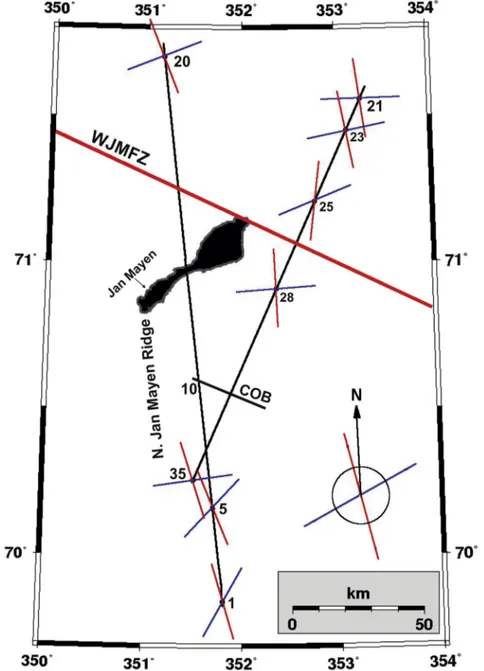
instruments are plotted inFig. 14. Theﬁgure does not provide the anisotropy directions exactly at the instrument locations, since the shear wave phases studied sample a large section of the proﬁle. This implies that the OBSs located to the north of the WJMFZ to a large extent provide anisotropy estimates of the Icelandic type crust south of the WJMFZ.

The anisotropy value ANI depends on which model layers the analyzed PSS waves have propagated in. Most PSS arrivals have penetrated as deep as the lower crust (OBS 21, 23, 25, 28 and 35), and in one case the modeled PSS arrival has propagated into the upper the mantle (OBS 20). In two cases, the analyzed PSS phases did not penetrate below the upper continental crust (OBS 1 and 5).

The PSS phases from the upper crust demonstrate anisotropy of 5e8 %, while the phases sampling the lower crust and mantle infer lower anisotropy - between 1 and 3%. This implies an average crustal anisotropy of about 3%.

A signiﬁcant portion of the phases used in the hodogram analysis have propagated through the continental crust (OBS 1, 5, 35;

Fig. 14). The results suggest the presence of S-wave anisotropy with the fast component along the Jan Mayen Ridge. This pattern of anisotropy is most readily interpreted as dikes striking along the ridge. This trend of dyke formation may to a large extent be controlled by pre-existing along-ridge zones of weakness. This interpretation is supported by the high Vp/Vs-ratios observed along this portion of the ridge, indicating the presence of maﬁc intrusions.

The majority of the phases used in the hodogram analysis have propagated dominantly through the Icelandic type oceanic crust (OBS 20, 21, 23, 25, 28;Fig. 14). The results are also within this ridge segment consistent with dikes intruded along the ridge, supporting the leaky transform hypothesis described byGernigon et al. (2009) andKandilarov et al. (2012).

Fig. 14.Map of the surveyed area with the azimuths of the fast (red lines) and slow (blue lines) anisotropy directions determined from the particle diagram analysis of 8 OBSs. OBS numbers are indicated along the lines. Note that the anisotropy directions are not obtained vertically below the instruments, but along the ray-paths studied (see text andTable 2 for details). The average fast and slow anisotropy directions are shown in the lower right corner of the map. WJMFZ: West Jan Mayen Fracture Zone. COB: Continent-Ocean- Boundary. (For interpretation of the references to colour in thisﬁgure legend, the reader is referred to the web version of this article.)

(17)

The largest anisotropy is inferred from the hodograms of PSS waves propagating in the upper crust. This indicates that the major contribution to the crustal anisotropy comes from dikes in the upper crust, which is in agreement with general models for oceanic crustal formation (e.g.White et al., 1992).

An alternative interpretation invoking the presence of prefer- entially aligned micro-cracks related to the present-day stressﬁeld (e.g.Crampin, 1990), is not supported by the focal mechanisms of local earthquakes, as these dominantly result from strike-slip movements along the WJMFZ (Havskov and Atakan, 1991;

Sørensen et al., 2007).

7. Conclusions

Controlled source OBS-data from the northern Jan Mayen Ridge have been modeled with regard to S-wave travel-times observed on the horizontal channels. The modeling was based on previous models derived from integrated use of MCS-data, OBS P-waves (vertical channel), and gravity data (Kandilarov et al., 2012). The mainﬁndings are as follows:

- The high Vp/Vs-ratios of 2.5e8.0 in the Cenozoic sediments along both lines are indicative of a low degree of consolidation and high porosity.

- The Vp/Vs-ratios of 1.9e2.2 in the Mesozoic and Paleozoic sequences on the continental part of the ridge are indicative of shale dominated lithology. The shale content on the ridge is higher than along the conjugate mid-Norwegian margin, and the shale content appears to increase northwards on the ridge.

- The S-wave modeling conﬁrms that the northernmost part of the Jan Mayen Ridge most readily can be interpreted as an Ice- landic type oceanic plateau, bordered to the north by thicker than normal oceanic crust derived from the Mohns ridge spreading system.

- The relatively high Vp/Vs-ratios of 1.85 modeled for oceanic layer 3 formed at the Mohns Ridge might indicate the presence of some amounts of serpentinized peridotites in the lower crust.

- On the northernmost part of the ridge, Vp/Vs-ratios of 1.85e1.9 are modeled in oceanic layer 3A. These values are similar to those obtained from the high-temperature neo-volcanic zone in northern Iceland.

- Signiﬁcantly lower Vp/Vs-ratios of around 1.75 are modeled in oceanic layer 3B along the easternﬂank of the ridge. This value may be interpreted as high Mg gabbros derived from elevated temperature melt, subject to normal present-day temperatures.

- Analyzes of particle diagrams suggests the presence of S-wave anisotropy with the fast component along the Jan Mayen Ridge.

This pattern of anisotropy is most readily interpreted as dikes intruded along the ridge, supporting the leaky transform hypothesis (e.g.Gernigon et al., 2009).

Acknowledgments

We would like to thank the crew of RV G.O. Sars and the engi- neers from the University of Bergen and GEOMAR for their assis- tance during the survey. The authors also want to thank Thomas Raum for guidance during the OBS modeling, and the Norwegian Petroleum Directorate, University of Bergen, the Norwegian Research Council (Petromaks program) and the European Union through the Transnational Access program (grant RITA-CT-2004- 505322 to IFM-GEOMAR) for the financial support. The finally thank Beata Mjelde for drawingfigures.

References

Allen, R.M., Nolet, G., Morgan, W.J., Vogfjord, K., Nettles, M., Ekstrom, G., Bergsson, B., Erlendsson, P., Foulger, G.R., Jakobsdottir, S., Julian, B.R., Pritchard, M., Ragnarsson, S., Stefansson, R., 2002. Plume-driven plumbing and crustal formation of Iceland. J. Geophys. Res. 107 (B8), 2163.

Bjarnason, I., Menke, W., Flovenz, O., Caress, D., 1993. Tomographic image of the mid-atlantic plate boundary is southwestern Iceland. J. Geophys. Res. 98 (B4), 6607e6622.

Brandsdottir, B., Menke, W., Einarsson, P., White, R., 1997. Faroe-iceland ridge experiment 2. Crustal structure of the kraﬂa central volcano. J. Geophys. Res.

104 (B4), 7867e7886.

Breivik, A.J., Mjelde, R., Grogan, P., Shimamura, H., Murai, Y., Nishimura, Y., 2005.

Caledonite development offshore-onshore svalbard based on ocean bottom seismometer, conventional seismic, and potentialﬁeld data. Tectonophysics 401, 79e117.

Breivik, A.J., Mjelde, R., Faleide, J.I., Murai, Y., 2012. The eastern Jan Mayen microcontinent volcanic margin. Geophys. J. Int. 188, 798e818.

Bromirski, P.D., Frazer, L.N., Dunnebier, F.K., 1990. Sediment shear Q from airgun OBS data. Geophys. J. Int. 110, 465e485.

Cande, S.C., Kent, D.V., 1995. Revised calibration of the geomagnetic polarity timescale for the late cretaceous and cenozoic. J. Geophys. Res. 100 (B4), 6093e6095.

Carlson, R., Miller, D.J., 1997. A new assessment of the abundance of serpentinite in the oceanic crust. Geophys. Res. Lett. 24 (4), 457e460.

Christensen, N., 1996. Poisson's ratio and crustal seismology. J. Geophys. Res. 101 (B2), 3139e3156.

Chung, T.W., Hirata, N., Sato, R., 1990. Two-dimensional P- and S-wave velocity structure of the yamato basin, the southern Japan sea from refraction data collected by an ocean bottom seismograph array. J. Phys. Earth 38, 99e147.

Crampin, S., 1990. The scattering of S-waves in the crust. Pageoph 132, 67e91.

Darbyshire, F., Bjarnason, I.T., White, R.S., Flovenz, O.G., 1998. Crustal structure above the Iceland mantle plume imaged by the ICEMELT refraction proﬁle.

Geophys. J. Int. 135, 1131e1149.

Digranes, P., Mjelde, R., Kodaira, S., Shimamura, H., Kanazwa, T., Shiobara, H., Berg, E.W., 1996. Modelling shear waves in OBS data from the Vøring basin (Northern Norway) by 2-D ray-tracing. Pageoph 147 (4), 611e629.

Domenico, S.N., 1984. Rock lithology and porosity determination from shear and compressional wave velocity. Geophysics 49 (8), 1188e1195.

Eldholm, O., Thiede, J., Taylor, E., 1989. Evolution of the Vøring volcanic margin. In:

Proceedings ODP, Scientiﬁc Results, vol. 104. Ocean Drilling Program, College Station, TX, pp. 1033e1065.

Gernigon, L., Olesen, O., Ebbing, J., Wienecke, S., Gaina, C., Mogaard, J.O., Sand, M., Myklebust, R., 2009. Geophysical insights and early spreading history in the vicinity of the Jan Mayen fracture zone, Norwegian-Greenland Sea. Tectono- physics 468, 185e205.

Gudlaugsson, S.T., Gunnarsson, M., Sand, M., Skogseid, J., 1988. Tectonic and volcanic events at the Jan Mayen Ridge microcontinent. Geological Soc. Lond.

Special Publ. 39, 85e93.http://dx.doi.org/10.1144/GSL.SP.1988.039.01.09.

Gudmundsson, O., 2003. The dense root of the Iceland crust. Earth Planet. Sci. Lett.

206, 427e440.http://dx.doi.org/10.1016/S0012-821X(02)01110-X.

Havskov, J., Atakan, K., 1991. Seismicity and volcanism of jan mayen island, Norway.

Terra Nova 3, 517e526.

Holbrook, W.S., Mooney, W.D., Christensen, N.J., 1992. Seismic velocity structure of the deep continental crust. In: Fountain, D., Arculus, R., Kay, R.W. (Eds.), Con- tinental Lower Crust. Elsevier, Amsterdam, pp. 451e464.

Kampfmann, W., Berckhemer, H., 1985. High-temperature experiments on the elastic and anelastic behavior of magmatic rocks. Earth Planet. Sci. Lett. 40, 223e247.

Kandilarov, A., Mjelde, R., Pedersen, R.-B., Hellevang, B., Papenberg, C., Petersen, C.- J., Planert, L., Flueh, E., 2012. The Northern boundary of the Jan Mayen microcontinent, North Atlantic determined from ocean bottom seismic, multichannel seismic, and gravity data. Mar. Geophys. Res. 33 (1), 55e76.http://dx.doi.org/

10.1007/s11001-012-9146-4.

Kodaira, S., Mjelde, R., Shimamura, H., Gunnarsson, K., Shiobara, H., 1997. Crustal structure of the Kolbeinsey ridge, N. Atlantic, obtained by use of Ocean bottom seismographs. J. Geophys. Res. 102, 3131e3151.

Kodaira, S., Mjelde, R., Gunnarsson, K., Shiobara, H., Shimamura, H., 1998. Structure of the Jan Mayen microcontinent and implications on its evolution. Geophys. J.

Int. 132, 383e400.

Menke, W., West, M., Brandsdottir, B., Sparks, D., 1998. Compressional and shear velocity structure of the lithosphere in northern Iceland. Bull. Seismol. Soc. Am.

88 (6), 1561e1571.

Mjelde, R., Timenes, T., Shimamura, H., Kanazawa, T., Shiobara, H., Kodaira, S., Nakainshi, A., 2002a. Acquisition, processing and analysis of densely sampled P- and S-wave OBS data on the mid-Norwegian Margin, NE Atlantic. Earth Planets Space 54, 1219e1236.

Mjelde, R., Fjellanger, J.P., Raum, T., Digranes, P., Kodaira, S., Breivik, A., Shimamura, H., 2002b. Where do P-S conversions occur? Analysis of OBS-data from the NE Atlantic Margin. First Break 20 (3), 153e160.

Mjelde, R., Aurvåg, R., Kodaira, S., Shimamura, H., Gunnarsson, K., Nakanishi, A., Shiobara, H., 2002c. Vp/Vs-ratios from the central Kolbeinsey Ridge to the Jan Mayen Basin, North Atlantic; implications on lithology, porosity, and present- day stressﬁeld. Mar. Geophys. Res. 23, 125e145.

(18)

Mjelde, R., Raum, T., Digranes, P., Shimamura, H., Shiobara, H., Kodaira, S., 2003. Vp/Vs-ratio along the Vøring Margin, NE Atlantic, derived from OBS data: implications on lithology and stress ﬁeld. Tectonophysics 369, 175e197.

Mjelde, R., Raum, T., Myhren, B., Shimamura, H., Murai, Y., Takanami, T., Karpuz, R., Næss, U., 2005. Continent-ocean transition on the Vøring Plateau, NE Atlantic, derived from densely sampled ocean bottom seismometer data. J. Geophys. Res.

110, B05101.http://dx.doi.org/10.1029/2004JB003026.

Mjelde, R., Eckhoff, I., Solbakken, S., Kodaira, S., Shimamura, H., Gunnarsson, K., Nakanishi, A., Shiobara, H., 2007. Gravity and S-wave modeling across the Jan Mayen Ridge, North Atlantic; implications for crustal lithology. Mar. Geophys.

Res. 28, 27e41.

Mjelde, R., Breivik, A.J., Raum, T., Mittelstaedt, E., Ito, G., Faleide, J.I., 2008a.

Magmatic and tectonic evolution of the North Atlantic. J. Geological Soc. Lond.

165, 31e42.

Mjelde, R., Raum, T., Breivik, A.J., Faleide, J.I., 2008b. Crustal transect along the North Atlantic. Mar. Geophys. Res. 29, 73e87.http://dx.doi.org/10.1007/s11001-008- 9046-9.

Mjelde, R., Raum, T., Kandilarov, A., Murai, Y., Takanami, T., 2009. Crustal structure and evolution of the outer Møre Margin, NE Atlantic. Tectonophysics 468, 224e243.http://dx.doi.org/10.1016/j.tecto.2008.06.003.

Mjelde, R., Goncharov, A., Muller, R.D., 2012. The Moho: boundary above upper mantle peridotites or lower crustal eclogites? A global review and new interpretations for passive margins. Tectonophysics 609, 636e650. http://

dx.doi.org/10.1016/j.tecto.2012.03.001.

Mosar, J., Eide, E.A., Osmundsen, P.T., Sommaruga, A., Torsvik, T.H., 2002. Greenland- Norway separation: a geodynamic model for the North Atlantic. Nor. J. Geology 82, 281e298.

Myhre, A., Eldholm, O., Sundvor, E., 1984. The Jan Mayen Ridge: present status. Polar Res. 2 (1), 47e59.

Pedersen, R.B., Thorseth, I.H., Nygaard, T.-.E., Lilley, M., Kelley, D., 2010. Hydro- thermal activity along the arctic mid-ocean ridge. In: Rona, P., et al. (Eds.), Di- versity of Hydrothermal, Systems on Slow Spreading Ocean Ridges, AGU Geophysical Monograph Series, 108, pp. 67e98.

Sigmundsson, F., 2006. Iceland geodynamics: Crustal Deformation and Divergent plate Tectonics. Springer, Berlin. ISBN: 10: 3e540-24165-5.

Sørensen, M.B., Ottem€oller, L., Havskov, J., Atakan, K., Hellevang, B., Pedersen, R.B., 2007. Tectonic processes in the jan mayen fracture zone based on earthquake occurrence and bathymetry. Bull. Seismol. Soc. Am. 97 (3), 772e779.http://

dx.doi.org/10.1785/0120060025.

Staples, R., White, R.S., Brandsdottir, B., Menke, W., Maguire, P.K.H., McBride, J.H., 1997. Faroe_Iceland ridge experiment 1. Crustal structure of northeastern Ice- land. J. Geophys. Res. 102 (B4), 7849e7866.

Stein, S., Wysession, M., 2003. An Introduction to Seismology, Earthquakes, and earth Structure. Blackwell Publishing, ISBN 0-86542-078-5.

Talwani, M., Eldholm, O., 1977. Evolution of the Norwegian-Greenland sea.

Geological Soc. Am. Bull. 88, 969e999.

Tessensohn, F., Piepjohn, K., 2000. Eocene compressive deformation in arctic Can- ada, north greenland and svalbard and its plate tectonic causes. Polarforschung 68, 121e124.

Torsvik, T.H., Van der Voo, R., Meert, J., Mosar, J., Walderhaug, H.J., 2001. Re- constructions of the continents around the North Atlantic at about the 60th parallel. Earth Planet. Sci. Lett. 187, 55e69.

White, R.S., McKenzie, D., O'Nions, R.K., 1992. Oceanic crustal thickness from seismic measurements and rare earth element inversions. J. Geophys. Res. 97, 19683e19715.

White, R., McKenzie, D., 1989. Magmatism at rift zones: the generation of volcanic continental margins andﬂood basalts. J. Geophys. Res. 94, 7685e7729.

Zelt, C.A., Smith, R.B., 1992. Seismic traveltime inversion for 2-D crustal velocity structure. Geophys. J. Int. 108, 16e34.

Zelt, C.A., Ellis, R.M., 1988. Practical and efﬁcient ray tracing in two-dimensional media for rapid traveltime and amplitude forward modelling. Can. J. Explor.

Geophys. 24, 16e31.

Zelt, C.A., 1999. Modelling strategies and model assessment for wide angle seismic traveltime data. Geophys. J. Int. 139, 183e204.

Zelt, C.A., Sain, K., Naumenko, J.V., Sawyer, D.S., 2003. Assessment of crustal velocity models using seismic refraction and reﬂection tomography. Geophys. J. Int. 153, 609e626.