Kernel-Based Object Tracking
Dorin Comaniciu Visvanathan Ramesh Peter Meer
Real-Time Vision and Modeling Department Siemens Corporate Research
755 College Road East, Princeton, NJ 08540
Electrical and Computer Engineering Department Rutgers University
94 Brett Road, Piscataway, NJ 08854-8058
Abstract
A new approach toward target representation and localization, the central component in visual track- ing of non-rigid objects, is proposed. The feature histogram based target representations are regularized by spatial masking with an isotropic kernel. The masking induces spatially-smooth similarity functions suitable for gradient-based optimization, hence, the target localization problem can be formulated us- ing the basin of attraction of the local maxima. We employ a metric derived from the Bhattacharyya coefficient as similarity measure, and use the mean shift procedure to perform the optimization. In the presented tracking examples the new method successfully coped with camera motion, partial occlusions, clutter, and target scale variations. Integration with motion filters and data association techniques is also discussed. We describe only few of the potential applications: exploitation of background information, Kalman tracking using motion models, and face tracking.
Keywords: non-rigid object tracking; target localization and representation; spatially-smooth sim- ilarity function; Bhattacharyya coefficient; face tracking.
1 Introduction
Real-time object tracking is the critical task in many computer vision applications such as surveil- lance [44, 16, 32], perceptual user interfaces [10], augmented reality [26], smart rooms [39, 75, 47], object-based video compression [11], and driver assistance [34, 4].
Two major components can be distinguished in a typical visual tracker. Target Representa- tion and Localization is mostly a bottom-up process which has also to cope with the changes in the appearance of the target. Filtering and Data Association is mostly a top-down process dealing with the dynamics of the tracked object, learning of scene priors, and evaluation of different hy- potheses. The way the two components are combined and weighted is application dependent and plays a decisive role in the robustness and efficiency of the tracker. For example, face tracking in
a crowded scene relies more on target representation than on target dynamics [21], while in aerial video surveillance, e.g., [74], the target motion and the ego-motion of the camera are the more important components. In real-time applications only a small percentage of the system resources can be allocated for tracking, the rest being required for the preprocessing stages or to high-level tasks such as recognition, trajectory interpretation, and reasoning. Therefore, it is desirable to keep the computational complexity of a tracker as low as possible.
The most abstract formulation of the filtering and data association process is through the state space approach for modeling discrete-time dynamic systems [5]. The information characterizing the target is defined by the state sequence
, whose evolution in time is specified by the dynamic equation
! "#
. The available measurements
$%
are related to the corresponding states through the measurement equation
$&(')*+!,)#
. In general, both
!
and
'-
are vector-valued, nonlinear and time-varying functions. Each of the noise sequences,
"
and
,)
is assumed to be independent and identically distributed (i.i.d.).
The objective of tracking is to estimate the state
given all the measurements
$/.
up that moment, or equivalently to construct the probability density function (pdf) 0
*1$2/.%#
. The theoretically optimal solution is provided by the recursive Bayesian filter which solves the problem in two steps. The prediction step uses the dynamic equation and the already computed pdf of the state at time3
547698
, 0
1$2/.#
, to derive the prior pdf of the current state,0
*1$2/.:#
. Then, the update step employs the likelihood function 0
;$%1#
of the current measurement to compute the posterior pdf0
+1$/.
).
When the noise sequences are Gaussian and
and
'<
are linear functions, the optimal solution is provided by the Kalman filter [5, p.56], which yields the posterior being also Gaussian.
(We will return to this topic in Section 6.2.) When the functions
=
and
')
are nonlinear, by linearization the Extended Kalman Filter (EKF) [5, p.106] is obtained, the posterior density being still modeled as Gaussian. A recent alternative to the EKF is the Unscented Kalman Filter (UKF) [42] which uses a set of discretely sampled points to parameterize the mean and covariance of the posterior density. When the state space is discrete and consists of a finite number of states, Hidden Markov Models (HMM) filters [60] can be applied for tracking. The most general class of filters is represented by particle filters [45], also called bootstrap filters [31], which are based on Monte Carlo integration methods. The current density of the state is represented by a set of
random samples with associated weights and the new density is computed based on these samples and weights (see [23, 3] for reviews). The UKF can be employed to generate proposal distributions for particle filters, in which case the filter is called Unscented Particle Filter (UPF) [54].
When the tracking is performed in a cluttered environment where multiple targets can be present [52], problems related to the validation and association of the measurements arise [5, p.150]. Gating techniques are used to validate only measurements whose predicted probability of appearance is high. After validation, a strategy is needed to associate the measurements with the current targets. In addition to the Nearest Neighbor Filter, which selects the closest measure- ment, techniques such as Probabilistic Data Association Filter (PDAF) are available for the single target case. The underlying assumption of the PDAF is that for any given target only one mea- surement is valid, and the other measurements are modeled as random interference, that is, i.i.d.
uniformly distributed random variables. The Joint Data Association Filter (JPDAF) [5, p.222], on the other hand, calculates the measurement-to-target association probabilities jointly across all the targets. A different strategy is represented by the Multiple Hypothesis Filter (MHF) [63, 20], [5, p.106] which evaluates the probability that a given target gave rise to a certain measurement sequence. The MHF formulation can be adapted to track the modes of the state density [13]. The data association problem for multiple target particle filtering is presented in [62, 38].
The filtering and association techniques discussed above were applied in computer vision for various tracking scenarios. Boykov and Huttenlocher [9] employed the Kalman filter to track vehicles in an adaptive framework. Rosales and Sclaroff [65] used the Extended Kalman Filter to estimate a 3D object trajectory from 2D image motion. Particle filtering was first introduced in vision as the Condensation algorithm by Isard and Blake [40]. Probabilistic exclusion for tracking multiple objects was discussed in [51]. Wu and Huang developed an algorithm to integrate multiple target clues [76]. Li and Chellappa [48] proposed simultaneous tracking and verification based on particle filters applied to vehicles and faces. Chen et al. [15] used the Hidden Markov Model formulation for tracking combined with JPDAF data association. Rui and Chen proposed to track the face contour based on the unscented particle filter [66]. Cham and Rehg [13] applied a variant of MHF for figure tracking.
The emphasis in this paper is on the other component of tracking: target representation and localization. While the filtering and data association have their roots in control theory, algorithms
for target representation and localization are specific to images and related to registration methods [72, 64, 56]. Both target localization and registration maximizes a likelihood type function. The difference is that in tracking, as opposed to registration, only small changes are assumed in the location and appearance of the target in two consecutive frames. This property can be exploited to develop efficient, gradient based localization schemes using the normalized correlation criterion [6]. Since the correlation is sensitive to illumination, Hager and Belhumeur [33] explicitly mod- eled the geometry and illumination changes. The method was improved by Sclaroff and Isidoro [67] using robust M-estimators. Learning of appearance models by employing a mixture of stable image structure, motion information and an outlier process, was discussed in [41]. In a differ- ent approach, Ferrari et al. [26] presented an affine tracker based on planar regions and anchor points. Tracking people, which rises many challenges due to the presence of large 3D, non-rigid motion, was extensively analyzed in [36, 1, 30, 73]. Explicit tracking approaches of people [69]
are time-consuming and often the simpler blob model [75] or adaptive mixture models [53] are also employed.
The main contribution of the paper is to introduce a new framework for efficient tracking of non-rigid objects. We show that by spatially masking the target with an isotropic kernel, a spatially- smooth similarity function can be defined and the target localization problem is then reduced to a search in the basin of attraction of this function. The smoothness of the similarity function allows application of a gradient optimization method which yields much faster target localization compared with the (optimized) exhaustive search. The similarity between the target model and the target candidates in the next frame is measured using the metric derived from the Bhattacharyya coefficient. In our case the Bhattacharyya coefficient has the meaning of a correlation score. The new target representation and localization method can be integrated with various motion filters and data association techniques. We present tracking experiments in which our method successfully coped with complex camera motion, partial occlusion of the target, presence of significant clutter and large variations in target scale and appearance. We also discuss the integration of background information and Kalman filter based tracking.
The paper is organized as follows. Section 2 discusses issues of target representation and the importance of a spatially-smooth similarity function. Section 3 introduces the metric derived from the Bhattacharyya coefficient. The optimization algorithm is described in Section 4. Experimental results are shown in Section 5. Section 6 presents extensions of the basic algorithm and the new
approach is put in the context of computer vision literature in Section 7.
2 Target Representation
To characterize the target, first a feature space is chosen. The reference target model is represented by its pdf > in the feature space. For example, the reference model can be chosen to be the color pdf of the target. Without loss of generality the target model can be considered as centered at the spatial location ? . In the subsequent frame a target candidate is defined at location @ , and is characterized by the pdf 0
@ #
. Both pdf-s are to be estimated from the data. To satisfy the low computational cost imposed by real-time processing discrete densities, i.e.,A -bin histograms should be used. Thus we have
target model: CB
D
B
>E
E
F
F
E
B
>E G8
target candidate: HB
@
#IJ
B
0KE @
#L
E
F F
E
B
0KE M8ON
The histogram is not the best nonparametric density estimate [68], but it suffices for our purposes.
Other discrete density estimates can be also employed.
We will denote by
B
P @
#OQ
PSR
B
H @
#L
B
C<T
(1) a similarity function betweenHB andCB . The functionPB
@ #
plays the role of a likelihood and its local maxima in the image indicate the presence of objects in the second frame having representations similar toCB defined in the first frame. If only spectral information is used to characterize the target, the similarity function can have large variations for adjacent locations on the image lattice and the spatial information is lost. To find the maxima of such functions, gradient-based optimization pro- cedures are difficult to apply and only an expensive exhaustive search can be used. We regularize the similarity function by masking the objects with an isotropic kernel in the spatial domain. When the kernel weights, carrying continuous spatial information, are used in defining the feature space representations,PB
@ #
becomes a smooth function in@ .
2.1 Target Model
A target is represented by an ellipsoidal region in the image. To eliminate the influence of different target dimensions, all targets are first normalized to a unit circle. This is achieved by independently rescaling the row and column dimensions withUWV andUYX .
Let
Z[\
[
]
be the normalized pixel locations in the region defined as the target model.
The region is centered at? . An isotropic kernel, with a convex and monotonic decreasing kernel profile
4)_^<#
1, assigns smaller weights to pixels farther from the center. Using these weights in- creases the robustness of the density estimation since the peripheral pixels are the least reliable, being often affected by occlusions (clutter) or interference from the background.
The function `ba"cedgf
+8<N\NN
A associates to the pixel at location
Z[
the index `
Z[#
of its bin in the quantized feature space. The probability of the featureh
8<N\NN
A in the target model is then computed as
B
>iE Jj
]
[
4)Lk=
Z[Wk
d
#il
R`
Z[\#m6
h T
(2) where
l
is the Kronecker delta function. The normalization constant
j
is derived by imposing the condition
FE
B
>E M8
, from where
jJ
8
][
4-ik= Z[Wk
d #
(3) since the summation of delta functions forh
M8-NNN
A is equal to one.
2.2 Target Candidates
Let
[ [
]on
be the normalized pixel locations of the target candidate, centered at@ in the current frame. The normalization is inherited from the frame containing the target model. Using the same kernel profile
4-p^<#
, but with bandwidth U , the probability of the featureh
8-NN\N
A in the target candidate is given by
B
0YE @
#IJjrq ]on
[
4 @
6s
[
U d l R`
[
#<6
h T
(4)
1The profile of a kernelt is defined as a functionubvxwy%z{}|*~D such thatt;|ui ) |.
where
jrq
8
]n
[
4-ikx
%K
q k d # (5)
is the normalization constant. Note that
jrq
does not depend on@ , since the pixel locations
[
are organized in a regular lattice and@ is one of the lattice nodes. Therefore,
jrq
can be precalculated for a given kernel and different values of U . The bandwidth U defines the scale of the target candidate, i.e., the number of pixels considered in the localization process.
2.3 Similarity Function Smoothness
The similarity function (1) inherits the properties of the kernel profile
4-p^<#
when the target model and candidate are represented according to (2) and (4). A differentiable kernel profile yields a differentiable similarity function and efficient gradient-based optimizations procedures can be used for finding its maxima. The presence of the continuous kernel introduces an interpolation process between the locations on the image lattice. The employed target representations do not restrict the way similarity is measured and various functions can be used forP . See [59] for an experimental evaluation of different histogram similarity measures.
3 Metric based on Bhattacharyya Coefficient
The similarity function defines a distance among target model and candidates. To accommodate comparisons among various targets, this distance should have a metric structure. We define the distance between two discrete distributions as
@
#r 8r6
PR
B
H @
#L
B
C<T
(6) where we chose
B
P @
#IQ
PR
B
H @
#L
B
C<T
F
E
B
0YE @ # B>iE
(7) the sample estimate of the Bhattacharyya coefficient betweenH andC [43].
The Bhattacharyya coefficient is a divergence-type measure [49] which has a straightforward geometric interpretation. It is the cosine of the angle between theA -dimensional unit vectors
B0
NNN
B0 F
and
B>
L\NNN!
B> F
. The fact thatH andC are distributions is thus explicitly
taken into account by representing them on the unit hypersphere. At the same time we can interpret (7) as the (normalized) correlation between the vectors
B0
iNN\N\
B0 F
and
B>
LN\NN\
B> F
. Properties of the Bhattacharyya coefficient such as its relation to the Fisher measure of information, quality of the sample estimate, and explicit forms for various distributions are given in [22, 43].
The statistical measure (6) has several desirable properties:
1. It imposes a metric structure (see Appendix). The Bhattacharyya distance [28, p.99] or Kullback divergence [19, p.18] are not metrics since they violate at least one of the distance axioms.
2. It has a clear geometric interpretation. Note that the < histogram metrics (including his- togram intersection [71]) do not enforce the conditions
FE
B
>E 98
and
FE
B
0KE M8
. 3. It uses discrete densities, and therefore it is invariant to the scale of the target (up to quanti-
zation effects).
4. It is valid for arbitrary distributions, thus being superior to the Fisher linear discriminant, which yields useful results only for distributions that are separated by the mean-difference [28, p.132].
5. It approximates the chi-squared statistic, while avoiding the singularity problem of the chi- square test when comparing empty histogram bins [2].
Divergence based measures were already used in computer vision. The Chernoff and Bhat- tacharyya bounds have been employed in [46] to determine the effectiveness of edge detectors. The Kullback divergence between joint distribution and product of marginals (e.g., the mutual informa- tion) has been used in [72] for registration. Information theoretic measures for target distinctness were discussed in [29].
4 Target Localization
To find the location corresponding to the target in the current frame, the distance (6) should be minimized as a function of@ . The localization procedure starts from the position of the target in
the previous frame (the model) and searches in the neighborhood. Since our distance function is smooth, the procedure uses gradient information which is provided by the mean shift vector [17].
More involved optimizations based on the Hessian of (6) can be applied [58].
Color information was chosen as the target feature, however, the same framework can be used for texture and edges, or any combination of them. In the sequel it is assumed that the following information is available: (a) detection and localization in the initial frame of the objects to track (target models) [50, 8]; (b) periodic analysis of each object to account for possible updates of the target models due to significant changes in color [53].
4.1 Distance Minimization
Minimizing the distance (6) is equivalent to maximizing the Bhattacharyya coefficientPB
@ #
. The search for the new target location in the current frame starts at the location@B of the target in the previous frame. Thus, the probabilities
B0YE B@
#L
E
F
of the target candidate at location @B in the current frame have to be computed first. Using Taylor expansion around the values0YEB
B@ #
, the linear approximation of the Bhattacharyya coefficient (7) is obtained after some manipulations as
PR
B
H @
#L
B
C-T+
8
F
E
B
0YE
B@ # B>iE
8
F
E
B
0YE
@ # B>E
B
0YE B
@ # N
(8) The approximation is satisfactory when the target candidate
B0YE @
#L
E
F
does not change drasti- cally from the initial
B0YE B@
#L
E
F
, which is most often a valid assumption between consecutive frames. The condition0YEB
B@
#
(or some small threshold) for allh
8-NN\N
A , can always be enforced by not using the feature values in violation. Recalling (4) results in
PR
B
H @
#L
B
C-T+
8
F
E
B
0YE B@ # B
>iE
jrq
] n
[
"
[ 4 @
6
[
U d
(9) where
[ F
E
B
>iE
B
0YE
B@ # l R`
[
#<6
h T N
(10) Thus, to minimize the distance (6), the second term in (9) has to be maximized, the first term being independent of @ . Observe that the second term represents the density estimate computed with kernel profile
4-p^<#
at@ in the current frame, with the data being weighted by
[
(10). The mode of this density in the local neighborhood is the sought maximum which can be found employing
the mean shift procedure [17]. In this procedure the kernel is recursively moved from the current location@B to the new location@B according to the relation
B
@
]n
[
[
[
@S
q d
]on
[
[
@m
q d
(11)
where
_^<#964 p^<#
, assuming that the derivative of
4-_^<#
exists for all
^&¡
R
o¢£#
, except for a finite set of points. The complete target localization algorithm is presented below.
Bhattacharyya CoefficientP¤RHB
@
#i
B
C<T
Maximization Given:
the target model
B>iE
E
F
and its location@B in the previous frame.
1. Initialize the location of the target in the current frame with @B , compute
B0YE B@
#L
E
F ,
and evaluate
P¤R
B
H B@
#i
B
C<T
FE
B
0YE B@ # B
>E
N
2. Derive the weights
[ [
]n
according to (10).
3. Find the next location of the target candidate according to (11).
4. Compute
B
0YE B@
#L
E
F
, and evaluate
P¤R
B
H B@
#i
B
C<T
FE
B
0YE B@ # B>E
N
5. While PRHB
B@
#L
B
C-T+¥ PR
B
H B@
#L
B
C<T
Do @B I¦
d B@ B@ #
Evaluate P¤RHB
B@
#L
B
C<T
6. If
k B@ 6 B@ k
¥J§ Stop.
Otherwise Set@B ¦ @B and go to Step 2.
4.2 Implementation of the Algorithm
The stopping criterion threshold§ used in Step 6 is derived by constraining the vectors@B and@B to be within the same pixel in original image coordinates. A lower threshold will induce subpixel accuracy. From real-time constraints (i.e., uniform CPU load in time), we also limit the number of mean shift iterations to ¨
FS©
V , typically taken equal to 20. In practice the average number of iterations is much smaller, about 4.
Implementation of the tracking algorithm can be much simpler than as presented above. The role of Step 5 is only to avoid potential numerical problems in the mean shift based maximization.
These problems can appear due to the linear approximation of the Bhattacharyya coefficient. How- ever, a large set of experiments tracking different objects for long periods of time, has shown that the Bhattacharyya coefficient computed at the new location@B failed to increase in only
KNª8!«
of the cases. Therefore, the Step 5 is not used in practice, and as a result, there is no need to evaluate the Bhattacharyya coefficient in Steps 1 and 4.
In the practical algorithm, we only iterate by computing the weights in Step 2, deriving the new location in Step 3, and testing the size of the kernel shift in Step 6. The Bhattacharyya coefficient is computed only after the algorithm completion to evaluate the similarity between the target model and the chosen candidate.
Kernels with Epanechnikov profile [17]
4-_^<#I
dY¬
#i8r6®^<#
if
^°¯M8
otherwise (12)
are recommended to be used. In this case the derivative of the profile,
_^<#
, is constant and (11) reduces to
B
@
]n
[
[ [
]n
[
[
(13) i.e., a simple weighted average.
The maximization of the Bhattacharyya coefficient can be also interpreted as a matched filtering procedure. Indeed, (7) is the correlation coefficient between the unit vectors
B
C and
B
H @ #
, representing the target model and candidate. The mean shift procedure thus finds the local maximum of the scalar field of correlation coefficients.
Will call the operational basin of attraction the region in the current frame in which the new location of the target can be found by the proposed algorithm. Due to the use of kernels this basin is at least equal to the size of the target model. In other words, if in the current frame the center of the target remains in the image area covered by the target model in the previous frame, the local maximum of the Bhattacharyya coefficient is a reliable indicator for the new target location. We assume that the target representation provides sufficient discrimination, such that the Bhattacharyya coefficient presents a unique maximum in the local neighborhood.
The mean shift procedure finds a root of the gradient as function of location, which can, however, also correspond to a saddle point of the similarity surface. The saddle points are unstable solutions, and since the image noise acts as an independent perturbation factor across consecutive frames, they cannot influence the tacking performance in an image sequence.
4.3 Adaptive Scale
According to the algorithm described in Section 4.1, for a given target model, the location of the target in the current frame minimizes the distance (6) in the neighborhood of the previous location estimate. However, the scale of the target often changes in time, and thus in (4) the bandwidth
U of the kernel profile has to be adapted accordingly. This is possible due to the scale invariance property of (6).
Denote byUY:±ª²ª³ the bandwidth in the previous frame. We measure the bandwidthUY´µ¶ in the current frame by running the target localization algorithm three times, with bandwidthsU
UY:±ª²ª³ ,
U
UY:±ª²ª³¸·¹U , and U
UY:±ª²ª³
6
·¹U . A typical value is ·¹U
ºKNª8
UW±µ²³ . The best result, UY´µ¶ ,
yielding the largest Bhattacharyya coefficient, is retained. To avoid over-sensitive scale adaptation, the bandwidth associated with the current frame is obtained through filtering
U ]
²»
¼
UY´µ¶+
i8r6®¼m#
UW±µ²³ (14)
where the default value for
¼
is 0.1. Note that the sequence ofU
]
²» contains important information about the dynamics of the target scale which can be further exploited.
4.4 Computational Complexity
Let N be the average number of iterations per frame. In Step 2 the algorithm requires to compute the representation
B0YE @
#i
E
F
. Weighted histogram computation has roughly the same cost as the unweighted histogram since the kernel values are precomputed. In Step 3 the centroid (13) is computed which involves a weighted sum of items representing the square-root of a division of two terms. We conclude that the mean cost of the proposed algorithm for one scale is approximately given by
jr½¾
¨
¬:¿
®À
q
¬Á
#
¨7À
q
¬Á
(15) where
¬:¿
is the cost of the histogram and
¬Á
the cost of an addition, a square-root, and a division.
We assume that the number of histogram entriesA and the number of target pixelsÀ
q
are in the same range.
It is of interest to compare the complexity of the new algorithm with that of target localization without gradient optimization, as discussed in [25]. The search area is assumed to be equal to the operational basin of attraction, i.e., a region covering the target model pixels. The first step is to computeÀ
q
histograms. Assume that each histogram is derived in a squared window ofÀ
q
pixels.
To implement the computation efficiently we obtain a target histogram and update it by sliding the windowÀ
q
times (
À q
horizontal steps times
À q
vertical steps). For each move
À q
additions are needed to update the histogram, hence, the effort is
¬:¿
À q À q
¬:Â
, where
¬:Â
is the cost of an addition. The second step is to computeÀ
q
Bhattacharyya coefficients. This can also be done by computing one coefficient and then updating it sequentially. The effort isA
¬Á
À q À q
¬Á
. The total effort for target localization without gradient optimization is then
jrÃĽÅ
¬:¿
À q À q
¬Â
A
À q À qo#
¬Á
À q À q
¬:Á
N
(16) The ratio between (16) and (15) is<Æ À
qKÇ
¨ . In a typical setting (as it will be shown in Section 5) the target has aboutÈ
IÉ
È
pixels (i.e.,
À q
È
) and the mean number of iterations is¨
ËÊKNª8!Ì
. Thus the proposed optimization technique reduces the computational timerÆ È
KÇÊoNª8Ì
Ê
times.
An optimized implementation of the new tracking algorithm has been tested on a 1GHz PC.
The basic framework with scale adaptation (which involves three optimizations at each step) runs at a rate of 150 fps allowing simultaneous tracking of up to five targets in real time. Note that without scale adaptations these numbers should be multiplied by three.
Figure 1: Football sequence, tracking player no. 75 . The frames 30, 75, 105, 140, and 150 are shown.
0 50 100 150
2 4 6 8 10 12 14 16 18
Frame Index
Mean Shift Iterations
Figure 2: The number of mean shift iterations function of the frame index for the Football se- quence. The mean number of iterations is
ÊoNª8Ì
per frame.
5 Experimental Results
The kernel-based visual tracker was applied to many sequences and it is integrated into several applications. Here we just present some representative results. In all but the last experiments the RGB color space was taken as feature space and it was quantized into
8Í}ÉD8ÍÎÉJ8!Í
bins. The algorithm was implemented as discussed in Section 4.2. The Epanechnikov profile was used for histogram computations and the mean shift iterations were based on weighted averages.
The Football sequence (Figure 1) has
8 È Ê
frames ofÏoÈ
É
Ê
pixels, and the movement of player no. 75 was tracked. The target was initialized with a hand-drawn elliptical region (frame
−40 0 −20 40 20
−20 −40 20 0
40 0.2
0.3 0.4 0.5 0.6 0.7 0.8 0.9 1
Y X
Bhattacharyya Coefficient
Initial location Convergence point
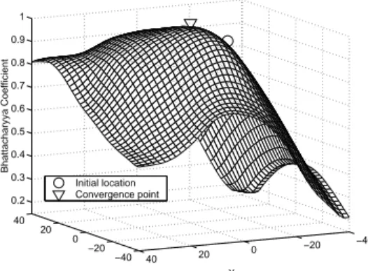
Figure 3: The similarity surface (values of the Bhattacharyya coefficient) corresponding to the rectangle marked in frame
8
È of Figure 1. The initial and final locations of the mean shift itera- tions are also shown.
Ï
) of sizeÐ
8gÉ
ÈoÏ (yielding normalization constants equal to
UYV
UYX
#Ñ
ÏÈ
Ío##
. The kernel- based tracker proves to be robust to partial occlusion, clutter, distractors (frame
8Êo
) and camera motion. Since no motion model has been assumed, the tracker adapted well to the nonstationary character of the player’s movements which alternates abruptly between slow and fast action. In addition, the intense blurring present in some frames due to the camera motion, does not influence the tracker performance (frame
8 È
). The same conditions, however, can largely perturb contour based trackers.
The number of mean shift iterations necessary for each frame (one scale) is shown in Fig- ure 2. The two central peaks correspond to the movement of the player to the center of the image and back to the left side. The last and largest peak is due to a fast move from the left to the right.
In all these cases the relative large movement between two consecutive frames puts more burden on the mean shift procedure.
To demonstrate the efficiency of our approach, Figure 3 presents the surface obtained by computing the Bhattacharyya coefficient for the Ò
8¹É
Ò 8
pixels rectangle marked in Figure 1, frame
8
È . The target model (the elliptical region selected in frameÏ
) has been compared with the target candidates obtained by sweeping in frame
8
È the elliptical region inside the rectangle.
The surface is asymmetric due to neighboring colors that are similar to the target. While most of the tracking approaches based on regions [7, 27, 50] must perform an exhaustive search in the rectangle to find the maximum, our algorithm converged in four iterations as shown in Figure 3.
Note that the operational basin of attraction of the mode covers the entire rectangular window.
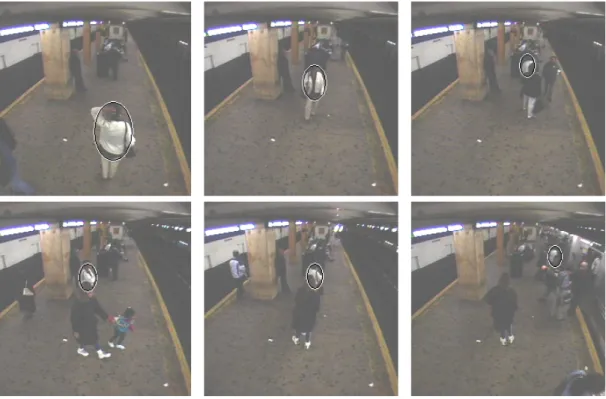
Figure 4: Subway-1 sequence. The frames 3140, 3516, 3697, 5440, 6081, and 6681 are shown.
30000 3500 4000 4500 5000 5500 6000 6500 7000 0.1
0.2 0.3 0.4 0.5 0.6 0.7
Frame Index
d
Figure 5: The minimum value of distance function of the frame index for the Subway-1 se- quence.
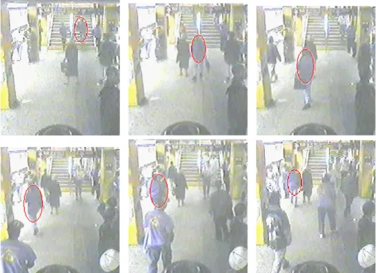
Figure 6: Subway-2 sequence. The frames 30, 240, 330, 450, 510, and 600 are shown.
In controlled environments with fixed camera, additional geometric constraints (such as the expected scale) and background subtraction [24] can be exploited to improve the tracking process.
The Subway-1 sequence ( Figure 4) is suitable for such an approach, however, the results presented here has been processed with the algorithm unchanged. This is a minute sequence in which a person is tracked from the moment she enters the subway platform till she gets on the train (about 3600 frames). The tracking is made more challenging by the low quality of the sequence due to image compression artifacts. Note the changes in the size of the tracked target.
The minimum value of the distance (6) for each frame, i.e., the distance between the target model and the chosen candidate, is shown in Figure 5. The compression noise elevates the residual distance value from
(perfect match) to a about
oN
Ï . Significant deviations from this value corre- spond to occlusions generated by other persons or rotations in depth of the target (large changes in the representation). For example, the
KN_Í
peak corresponds to the partial occlusion in frame
Ï
ÍoÌ
Ð . At the end of the sequence, the person being tracked gets on the train, which produces a complete occlusion.
The shorter Subway-2 sequence (Figure 6) of about 600 frames is even more difficult since
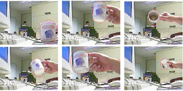
Figure 7: Mug sequence. The frames 60, 150, 240, 270, 360, and 960 are shown.
the camera quality is worse and the amount of compression is higher, introducing clearly visible artifacts. Nevertheless, the algorithm was still able to track a person through the entire sequence.
In the Mug sequence (Figure 7) of about 1000 frames the image of a cup (frame 60) was used as target model. The normalization constants were
UYV ËÊoÊK
UWX JÍoÊo#
. The tracker was tested for fast motion (frame 150), dramatic changes in appearance (frame 270), rotations (frame 270) and scale changes (frames 360-960).
6 Extensions of the Tracking Algorithm
We present three extensions of the basic algorithm: integration of the background information, Kalman tracking, and an application to face tracking. It should be emphasized, however, that there are many other possibilities through which the visual tracker can be further enhanced.
6.1 Background-Weighted Histogram
The background information is important for at least two reasons. First, if some of the target features are also present in the background, their relevance for the localization of the target is diminished. Second, in many applications it is difficult to exactly delineate the target, and its model might contain background features as well. At the same time, the improper use of the
background information may affect the scale selection algorithm, making impossible to measure similarity across scales, hence, to determine the appropriate target scale. Our approach is to derive a simple representation of the background features, and to use it for selecting only the salient parts from the representations of the target model and target candidates.
Let
B
Ó E E
F
(with
FE
B
Ó E Ô8
) be the discrete representation (histogram) of the back- ground in the feature space and ÓÕB be its smallest nonzero entry. This representation is computed in a region around the target. The extent of the region is application dependent and we used an area equal to three times the target area. The weights
Ö E
Ë×7ØÙ
B
ÓÕ
B
Ó E o8
E
F (17)
are similar in concept to the ratio histogram computed for backprojection [71]. However, in our case these weights are only employed to define a transformation for the representations of the target model and candidates. The transformation diminishes the importance of those features which have lowÖ E , i.e., are prominent in the background. The new target model representation is then defined by
B
>E Ëj
Ö E ]
[
4-ik=
Z[Yk
d
#il
R`
; Z[#<6
h T
(18) with the normalization constant
j
expressed as
j¸
8
][
4-Lk= Z[ k d # FE
Ö E l R` Z[ #<6
h T N
(19) Compare with (2) and (3). Similarly, the new target candidate representation is
B
0YE @
#OJjrq
Ö E ]on
[
4 @
6
[
U d l R`
[
#<6
h T
(20) where now
jrq
is given by
jrqg
8
] n
[
4-Lkx
%o
q k d # FE
Ö E l R`
[
#<6
h T N
(21)
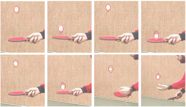
An important benefit of using background-weighted histograms is shown for the Ball se- quence (Figure 8). The movement of the ping-pong ball from frame to frame is larger than its size.
Applying the technique described above, the target model can be initialized with a
8gÉ
Ï 8
size region (frame 2), larger than one obtained by accurate target delineation. The larger region yields
Figure 8: Ball sequence. The frames 2, 12, 16, 26, 32, 40, 48, and 51 are shown.
a satisfactory operational basin of attraction, while the probabilities of the colors that are part of the background are considerably reduced. The ball is reliably tracked over the entire sequence of
Ío
frames.
The last example is also taken from the Football sequence. This time the head and shoulder of player no. È
Ì
is tracked (Figure 9). Note the changes in target appearance along the entire sequence and the rapid movements of the target.
6.2 Kalman Prediction
It was already mentioned in Section 1 that the Kalman filter assumes that the noise sequences
"
and
,-
are Gaussian and the functions
!
and
'-
are linear. The dynamic equation becomes
Ú¸ÛÜ
"
while the measurement equation is
$Ú¸ÝÞ
,)
. The matrix
Û
is called the system matrix and
Ý
is the measurement matrix. As in the general case, the Kalman filter solves the state estimation problem in two steps: prediction and update. For more details see [5, p.56].
The kernel-based target localization method was integrated with the Kalman filtering frame- work. For a faster implementation, two independent trackers were defined for horizontal and ver- tical movement. A constant-velocity dynamic model with acceleration affected by white noise
Figure 9: Football sequence, tracking player no. 59. The frames 70, 96, 108, 127, 140, 147 are shown.
[5, p.82] has been assumed. The uncertainty of the measurements has been estimated according to [55]. The idea is to normalize the similarity surface and represent it as a probability density function. Since the similarity surface is smooth, for each filter only 3 measurements are taken into account, one at the convergence point (peak of the surface) and the other two at a distance equal to half of the target dimension, measured from the peak. We fit a scaled Gaussian to the three points and compute the measurement uncertainty as the standard deviation of the fitted Gaussian.
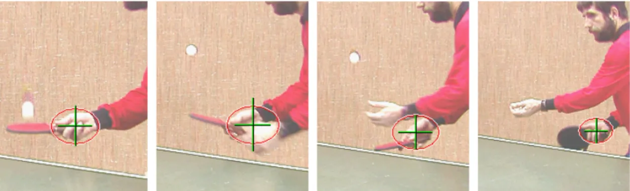
A first set of tracking results incorporating the Kalman filter is presented in Figure 10 for the 120 frames Hand sequence where the dynamic model is assumed to be affected by a noise with standard deviation equal toÈ . The size of the green cross marked on the target indicates the state uncertainty for the two trackers. Observe that the overall algorithm is able to track the target (hand) in the presence of complete occlusion by a similar object (the other hand). The presence of a similar object in the neighborhood increases the measurement uncertainty in frame 46, determining an increase in state uncertainty. In Figure 11a we present the measurements (dotted) and the estimated location of the target (continuous). Note that the graph is symmetric with respect to the number of frames since the sequence has been played forward and backward. The velocity associated with the two trackers is shown in Figure 11b.
A second set of results showing tracking with Kalman filter is displayed in Figure 12. The sequence has
8
ÒoÐ frames of Ï
}É
Êo
pixels each and the initial normalization constants were
Figure 10: Hand sequence. The frames 40, 46, 50, and 57 are shown.
0 20 40 60 80 100 120
190 200 210 220 230 240 250 260 270
Frame Index
Measurement and Estimated Location
0 20 40 60 80 100 120
−6
−4
−2 0 2 4 6
Frame Index
Estimated Velocity
(a) (b)
Figure 11: Measurements and estimated state for Hand sequence. (a) The measurement value (dotted curve) and the estimated location (continuous curve) function of the frame index. Upper curves correspond to the y filter, while the lower curves correspond to the x filter. (b) Estimated velocity. Dotted curve is for the y filter and continuous curve is for the x filter
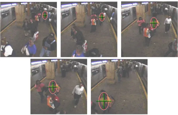
Figure 12: Subway-3 sequence: The frames 470, 529, 580, 624, and 686 are shown.
UYV
UWX
#ei88\K8
Ò #
. Observe the adaptation of the algorithm to scale changes. The uncertainty of the state is indicated by the green cross.
6.3 Face Tracking
We applied the proposed framework for real-time face tracking. The face model is an elliptical re- gion whose histogram is represented in the intensity normalizedß
space with
8 Ò É8
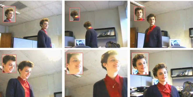
Ò bins. To adapt to fast scale changes we also exploit the gradient information in the direction perpendicular to the border of the hypothesized face region. The scale adaptation is thus determined by maxi- mizing the sum of two normalized scores, based on color and gradient features, respectively. In Figure 13 we present the capability of the kernel-based tracker to handle scale changes, the subject turning away (frame 150), in-plane rotations of the head (frame 498), and foreground/background saturation due to back-lighting (frame 576). The tracked face is shown in the small upper-left window.
Figure 13: Face sequence: The frames 39, 150, 163, 498, 576, and 619 are shown.
7 Discussion
The kernel-based tracking technique introduced in this paper uses the basin of attraction of the similarity function. This function is smooth since the target representations are derived from con- tinuous densities. Several examples validate the approach and show its efficiency. Extensions of the basic framework were presented regarding the use of background information, Kalman fil- tering, and face tracking. The new technique can be further combined with more sophisticated filtering and association approaches such as multiple hypothesis tracking [13].
Centroid computation has been also employed in [53]. The mean shift is used for tracking human faces by projecting the histogram of a face model onto the incoming frame [10]. However, the direct projection of the model histogram onto the new frame can introduce a large bias in the estimated location of the target, and the resulting measure is scale variant (see [37, p.262] for a discussion).
We mention that since its original publication in [18] the idea of kernel-based tracking has been exploited and developed forward by various researchers. Chen and Liu [14] experimented with the same kernel-weighted histograms, but employed the Kullback-Leibler distance as dissim- ilarity while performing the optimization based on trust-region methods. Haritaoglu and Flickner
[35] used an appearance model based on color and edge density in conjunction with a kernel tracker for monitoring shopping groups in stores. Yilmaz et al. [78] combined kernel tracking with global motion compensation for forward-looking infrared (FLIR) imagery. Xu and Fujimura [77] used night vision for pedestrian detection and tracking, where the detection is performed by a support vector machine and the tracking is kernel-based. Rao et al.[61] employed kernel tracking in their system for action recognition, while Caenen et al. [12] followed the same principle for texture analysis. The benefits of guiding random particles by gradient optimization are discussed in [70]
and a particle filter for color histogram tracking based on the metric (6) is implemented in [57].
Finally we would like to add a word of caution. The tracking solution presented in this paper has several desirable properties: it is efficient, modular, has straightforward implementation, and provides superior performance on most image sequences. Nevertheless, we note that this technique should not be applied blindly. Instead, the versatility of the basic algorithm should be exploited to integrate a priori information which is almost always available when a specific application is considered. For example, if the motion of the target from frame to frame is known to be larger than the operational basin of attraction, one should initialize the tracker in multiple locations in the neighborhood of basin of attraction, according to the motion model. If occlusions are present, one should employ a more sophisticated motion filter. Similarly, one should verify that the chosen target representation is sufficiently discriminant for the application domain. The kernel-based tracking technique, when combined with prior task-specific information, can achieve reliable performance. 2
APPENDIX
Proof that the distance
B
H B
C
#r 8r6
P B H B
C #
is a metric
The proof is based on the properties of the Bhattacharyya coefficient (7). According to the Jensen’s inequality [19, p.25] we have
P B H B
C
#<
F
E
B
0KE >iEB
F
E
B
0KE
B
>E
B
0YE
¯ F
E
B
>E à8\
(A.1)
2A patent application has been filed covering the tracking algorithm together with the extensions and various applications [79].