An extended lidar-based cirrus cloud retrieval scheme: first application over an Arctic site
K
ONSTANTINAN
AKOUDI,
1,2,*I
WONAS. S
TACHLEWSKA,
3 ANDC
HRISTOPHR
ITTER11Alfred Wegener Institute, Helmholtz Centre for Polar and Marine Research, Telegrafenberg A45 Potsdam, 14473, Germany
2Institute of Physics and Astronomy, University of Potsdam, Karl-Liebknecht 24/25, 14476, Potsdam, Germany
3Faculty of Physics, University of Warsaw (FUW), Warsaw 00-927, Poland
*konstantina.nakoudi@awi.de
Abstract: Accurate and precise characterization of cirrus cloud geometrical and optical proper- ties is essential for better constraining their radiative footprint. A lidar-based retrieval scheme is proposed here, with its performance assessed on fine spatio-temporal observations over the Arctic site of Ny-Ålesund, Svalbard. Two contributions related to cirrus geometrical (dynamic Wavelet Covariance Transform (WCT)) and optical properties (constrained Klett) are reported.
Thedynamic WCTrendered cirrus detection more robust, especially for thin cirrus layers that frequently remained undetected by the classical WCT method. Regarding optical characterization, we developed an iterative scheme for determining the cirrus lidar ratio (LRci) that is a crucial parameter for aerosol - cloud discrimination. Building upon the Klett-Fernald method, the LRci was constrained by an additionalreference value. In established methods, such as the double-ended Klett, an aerosol-freereference valueis applied. In the proposedconstrained Klett, however, the reference value was approximated from cloud-free or low cloud optical depth (COD up to 0.2) profiles and proved to agree with independent Raman estimates. For optically thin cirrus, theconstrained Klettinherent uncertainties reached 50% (60-74%) in terms of COD (LRci). However, for opaque cirrus COD (LRci) uncertainties were lower than 10%
(15%). The detection method discrepancies (dynamic versus static WCT) had a higher impact on the optical properties of low COD layers (up to 90%) compared to optically thicker ones (less than 10%). Theconstrained Klettpresented high agreement with two established retrievals.
For an exemplary cirrus cloud, theconstrained Klettestimated theCOD355(LR355ci ) at 0.28± 0.17 (29±4 sr), the double-ended Klett at 0.27±0.15 (32±4 sr) and the Raman retrievals at 0.22±0.12 (26±11 sr). Our approach to determine the necessaryreference valuecan also be applied in established methods and increase their accuracy. In contrast, the classical aerosol-free assumption led to 44 srLRcioverestimation in optically thin layers and 2-8 sr in thicker ones.
The multiple scattering effect was corrected using Eloranta (1998) and accounted for 50-60%
extinction underestimation near the cloud base and 20-30% within the cirrus layers.
© 2021 Optical Society of America under the terms of theOSA Open Access Publishing Agreement
1. Introduction
Cirrus clouds play a key role in the Earth radiative budget. Cirrus are the only cloud genus inducing either cooling or heating at the top of the atmosphere during daytime, with the rest of the clouds producing a cooling effect [1,2]. The relative magnitude of short-wave cooling and infrared warming is highly dependent on the cloud geometrical, optical and microphysical properties [3–5]. Cirrus clouds occur on an average frequency of 40% over the mid-latitudes [6], which maximizes over the tropics (up to 70%) [7] and decreases towards the poles. Arctic ice clouds display highly variable occurrence frequencies, from 25% over Ny-Ålesund, Svalbard, (single layer clouds) [8] up to 50% over Eureka, Nunavut, Canada [9]. However, there is a lack
#414770 https://doi.org/10.1364/OE.414770
Journal © 2021 Received 16 Nov 2020; revised 25 Dec 2020; accepted 11 Jan 2021; published 4 Mar 2021
of studies focusing on the coverage, geometrical and optical properties of solely Arctic cirrus clouds.
Accurate and precise cirrus cloud detection is of high necessity. Apart from affecting the Earth radiative budget [10], the geometrical cloud thickness is indispensable for parameterization schemes of cirrus cloud optical depth (COD) [11]. Cirrus optical properties have been globally assessed by collocated Cloud-Aerosol lidar with Orthogonal Polarization (CALIOP) and Cloud Profiling Radar measurements, yielding a quite stable cirrus lidar ratio (LRci, ratio of extinction (α) to backscatter coefficient(β) within the cirrus cloud range) of 33±5 sr over the ocean [12].
However, satellite observations over the poles were limited, with dedicated aircraft campaigns bringing added value through alternated lidar and in-situ cirrus cloud measurements [13]. Cirrus geometrical and optical properties have also been derived from the synergy of active and passive remote sensing [14–17]. Nevertheless, exploiting infrared radiances to detect ice clouds [18,19]
and retrieve their optical properties [20,21] is challenging over cold and bright surfaces such as snow and ice.
Lidar systems are capable of delivering vertically resolved geometrical and optical properties of optically thin clouds on fine spatio-temporal scales. Their operating wavelengths, i.e. at ultraviolet, visible and near infrared, are ideal for cirrus studies, as they are more sensitive to small crystal sizes compared to millimeter radar systems [22]. Lidar-relevant cirrus optical properties are the COD, the particulate linear depolarization ratio (LPDR, indicates the sphericity of ice crystals), the LR (indicates type of ice crystals) and the color ratio (CR, ratio of backscatter coefficients at two different wavelengths, indicates the size of ice crystals).
The accuracy of cloud optical properties is critical for high quality radiative effect estimates [23], cloud phase classification [24,25] and cloud – aerosol discrimination (CAD) [17,26–28]. Lofted dust and smoke layers transported into the Arctic, were miss-interpreted as ice clouds in previous CALIOP data releases and motivated their subsequent improvement [29–31]. Conversely, optically thin ice clouds are still frequently miss-classified as aerosols in the polar regions, although the latest CALIOP CAD algorithm has been significantly improved [31–33]. CALIOP cloud phase and CAD algorithms rely on LPDR and CR as a function of temperature, latitude and altitude [31,34]. Thus, ground-based lidar observations that provide similar optical parameters can provide a valuable validation for satellite lidar processing algorithms (e.g. currently CALIOP aboard CALIPSO [35] and imminently ATLID aboard EARTHCARE [36]).
Different lidar-based retrievals of cirrus cloud optical properties exist in literature, such as the transmittance [37–39], the double-ended Klett [40], the backward – total optical depth [41]
and the Raman technique [40]. Each of these retrievals has its own strengths and limitations.
For instance, the transmittance and backward – total optical depth methods cannot be applied to optically thin cirrus (COD<0.05 and COD<0.1, respectively). The Raman technique provides a vertically-dependentLRcibut is limited to night-time applications, contrary to the double-ended Klett method that, however, yields a layer-meanLRci.
In this study, we propose an extended cirrus cloud retrieval scheme, consisting of detection (dynamic WCT) and optical characterization (constrained Klett). The scheme is applied on representative cirrus clouds over Ny-Ålesund, Svalbard, and its limitations and strengths are investigated. Sensitivities related to cirrus detection are performed (section3) and their effect on cirrus optical properties is also examined (section4.3). The inherent uncertainties of the proposedconstrained Klettare also quantified (section4.2). Finally, theconstrained Klettis compared with two established optical retrievals, namely the double-ended Klett and Raman (section5), and their limitations and strengths are discussed (section6). The optical properties are corrected for the multiple scattering effect (Appendix). Cirrus layers are divided in three regimes according to their COD, following the classification of Sassen and Cho (1992) [42] i.e.
sub-visible (COD<0.03), optically-thin (0.03<COD<0.3) and opaque cirrus layers (0.3<
COD<3). Hereafter, the term cirrus cloud will refer to a set of consecutive cirrus layers.
2. Methods
2.1. Instrumentation and selection of cirrus clouds
In this work, we exploit a unique measurement dataset from the multi-wavelength Koldewey Aerosol Raman lidar (KARL) system, which is installed on the Alfred Wegener Institute – Institute Paul Emile Victor (AWIPEV) research base, Ny-Ålesund (78.9oN, 11.9oE), Svalbard Archipelago. KARL is a powerful so called 3β+2α+2δ+2wv system equipped with an Nd:YAG laser that emits pulses of 200 mJ at 1064, 532 and 355 nm with a 50 Hz repetition rate [43]. The receiver comprises a 70 cm diameter telescope with a 2.28 mrad field of view (FOV), while the laser beam divergence amounts to 0.8 mrad. The range of full overlap is 600 m.
The combination of photon counting (PC) and analog (A) acquisition mode allows for large dynamical detection range. The specifications of KARL enable high quality signal acquisition at fine vertical and temporal scales (7.5 m, 1.5 min), which are ideal for the investigation of cirrus cloud properties. KARL has been deployed for the evaluation of aerosol optical, microphysical and radiative properties using classical approaches [44–46] or in combination with airborne lidar [47]. However, cloud optical retrievals with KARL were so far underexplored [48].
This study focuses on cirrus clouds and, thus, the presence of supercooled liquid–water layers should be excluded. Therefore, we only considered clouds with temperature lower than -40oC, which is the homogeneous nucleation temperature, at the height of cloud base (Cbase) and cloud top (Ctop) [15,26]. Temperature profiles were obtained from radiosondes, which are daily launched at 11 UT from the AWIPEV research base [49–51]. The utilized temperature criterion is quite strong as Shupe (2011) [52] reported only 3-5% liquid water occurrence between -40 and -30oC within Arctic clouds. Thus, the possibility of liquid water presence is very low, even within the range of temperature uncertainty, i.e. sensor related uncertainties or errors due to radiosonde drift and temporal discrepancy with lidar observations.
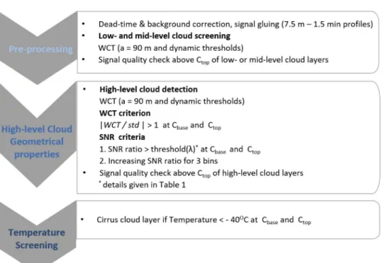
In the following section we present in detail all the steps of cirrus detection, including the revised method and its newly introduced parameters. In parallel, the main steps are depicted in Fig.1and Fig.2. Note that the code for the revised cirrus detection is publicly available [53].
2.2. Cirrus detection and underlying cloud screening
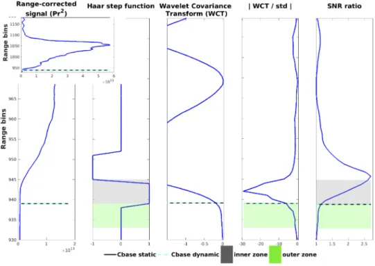
The Wavelet Covariance Transform (WCT) method [54] was extended with dynamic thresholds for detecting the cirrusCbaseandCtop. The classical WCT method is sensitive to lidar signal vertical gradients and has been employed for detecting either cirrus clouds [55,56] or the planetary boundary layer top height [57–59]. Firstly, the lidar signals were corrected for the dead-time, electronic noise and background illumination effects [43]. Then, the PC and A signal components were glued together as described in Hoffmann (2011) [43]. The gluing interval (several hundred meters zone) was selected as such that both signals were of high quality i.e. non-saturated PC and A with high SNR. Finally, the lidar range-corrected (Pr2) signal was normalized (with respect to the median signal between the range of full overlap and 12 km). The latter step was essential for making the WCT profiles comparable to those from literature [60] and did not affect thePr2 signal and WCT gradients. In Fig.1thePr2signal and WCT profiles corresponding to the lower part of a cirrus layer are presented. The WCT profile (Eq. (1)) can be perceived as the low-pass filtered version of thePr2signal [59] as it is based on the convolution of thePr2signal with a Haar step function (Eq. (2)) of specific step width (dilation,α) and step location (b).
Wf(α,b)= 1 α
∫ Ctop
Cbase
P(r) ·r2·h
(︃r−b
α )︃
dr (1)
h
(︃r−b
α )︃
=
⎧⎪
⎪⎪
⎨
⎪⎪
⎪
⎩
+1, b−α2 ≤r≤b
−1, b≤r≤b+α2 0, elsewhere
(2)
Fig. 1.Exemplary profiles ofPr2signal, Haar step function, WCT, WCT to signal standard deviation (std) ratio (
|︁
|︁
|︁
|︁
WCT/std
|︁
|︁
|︁
|︁) andSNR ratio, which correspond to the lower part of a cirrus layer observed at 7-9 km by KARL over Ny-Ålesund. Horizontal lines denote the dynamic (cyan) and static (black) derivedCbase. Grey (green) shaded areas denote the half dilation (a/2) zone within (outside) the cirrus layer. The whole cirrus layerPr2profile is given in the upper left inset figure. The signal std was calculated within the outer zone of each range bin.
ThePr2signal was integrated within half dilation (α/2) below (outer zone, Fig.1) and above (inner zone, Fig.1) each range bin. An appropriate dilation is crucial for accurate cirrus detection.
A relatively narrow dilation produces more noisy WCT profiles, while a too wide dilation may not resolve small-scale features such as thin clouds. In order to select an appropriate dilation, we assessed its effect on cirrus detection through a sensitivity analysis (section3.1).
The knowledge of cloud presence below the targeted cirrus layers is important. For this reason, underlying cloud layers were screened with the WCT method. If both theCbaseandCtopwere identified below 5 km (6 km), the cloud was flagged aslow-level(mid-level). It should be noted that the low-level Arctic ice clouds and ice fogs are not considered cirrus clouds [22]. Lidar profiles were retained for further evaluation on condition that signal quality was high. Otherwise, if the signal-to-noise ratio (SNR) was decreased (<3 as in [41]) above the low- or mid-level clouds, the profiles were discarded. Likewise, the signal quality was checked above the cirrus Ctop. The cirrus detection scheme is outlined in Fig.2.
2.2.1. Revised detection method: dynamic wavelet covariance transform
A crucial parameter for cirrus detection is the WCT threshold, which determines whether a signal gradient denotes a cirrus layer boundary or not. Static WCT thresholds have been proposed so far [60,61]. However, in this study we introduce dynamic thresholds, which assess the strength of the detected gradients with respect to the given signal variability. The dynamic thresholds
Fig. 2.Flowchart of newly proposed cirrus detection scheme. For details see section2.2.
The cirrus detection algorithm is given inCode 1[53].
depend on the ratio of WCT over the signal standard deviation (
|︁
|︁
|︁
|︁
WCT/std
|︁
|︁
|︁
|︁) as well as on the SNR. This dynamic approach has a higher robustness potential, since it is adaptable to the given cloud strength and lidar specifications. After examining a significant number of characteristic profiles, we found that cirrus peaks were related to WCT values exceeding the signal standard deviation (
|︁
|︁
|︁
|︁
WCT/std
|︁
|︁
|︁
|︁
>1, e.g. Fig.1).
|︁
|︁
|︁
|︁
WCT/std
|︁
|︁
|︁
|︁thresholds of 1.5 and 2 were also investigated, but they frequently detected only stronger cirrus parts, leaving out the faint marginal parts. In the upward (downward) direction, a candidateCbase(Ctop) was identified at one bin below (above) the range where
|︁
|︁
|︁
|︁
WCT/std
|︁
|︁
|︁
|︁
>1.
In order to discriminate cirrus related peaks from noise, an SNR related criterion was also introduced. At each range bin, the median SNR was calculated atα/2 bins below andα/2 bins above, whereαis the dilation of the WCT profile (Fig.1). More specifically, the median SNR was calculated within the inner and outer zones of bins, where
|︁
|︁
|︁
|︁
WCT/std
|︁
|︁
|︁
|︁
>1. Then, the algorithm checked whether the inner to outer zoneSNR ratioexceeded a given threshold in order to make sure that the detected peaks were not related to noise but to a real feature. The above mentioned procedure was performed in the upward (downward) direction forCbase(Ctop) detection. Additionally, an increasingSNR ratiowas demanded for three consecutive bins above theCbase(below theCtop). TheSNR ratiovalues were found to slightly differ for each wavelength due to differences in the SNR of each channel and are summarized in theAppendix. A more detailed investigation on the WCT wavelength dependency is presented in section3.2. An assessment of the dynamic thresholds in comparison to the static ones is presented in section3.3.
In the following section we describe in detail all the steps of the proposedconstrained Klett method (section2.3.2), including the newly introduced parameters, i.e. theconvergence range,
the estimated reference backscatter ratio (BSRref) as well as the recursiveLRciprocess and the factor used to adjust theLRciafter each iteration (Eq. (3)). Moreover, we depict the steps in Fig.4to outline the methodology. Note that we have made publicly available the code of the constrained Klett[53].
2.3. Cirrus optical characterization
2.3.1. Temporal averaging within stationary periods
High vertical (7.5 m) and temporal (1.5 min) resolution profiles allowed for reliable cirrus detection. However, the precision of optical properties was affected by statistical uncertainties (signal noise andreference value uncertainty) and, thus, temporal averaging was desirable.
Nonetheless, care should be taken with long temporal averaging to avoid smearing out the cloud physical variability i.e. to avoid averaging cloud and cloud-free range bins and produce physically unrealistic profiles. More importantly, distorted particulate extinction (αpart) profiles affect the accuracy of radiative effect estimates [23].
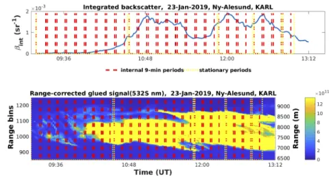
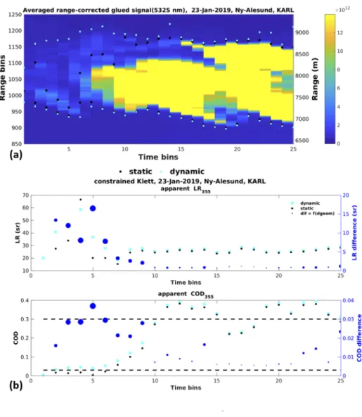
Bearing the aforementioned aspects in mind, we adopted a temporal averaging that is constrained by periods of stationarity following Lanzante (1996) [62]. This procedure is based on the Mann–Wilcoxon–Whitney test, such that the data points of one stationary period share the same COD statistical distribution [62]. This method has already been applied to time-series of cirrus COD and geometrical thickness by Larroza et al. (2013) [39]. In this study, the procedure was applied on the integrated backscatter coefficient (βint) time-series , which was obtained from an initial guess Klett-Fernald retrieval. The designation of stationary (yellow lines) and temporal (red lines) averaging periods is shown for the case of 23 January 2019 in Fig.3. The βintwas selected instead of the COD because the latter might be influenced by the assumedLRci. However, for the majority of the cirrus clouds analyzed over Ny-Ålesund (2011-2020) theβint and COD exhibited similar variability.
Fig. 3. Time-series of integrated backscatter (βint, upper panel) and height-time plot of Pr2 signal (lower panel) with overlaid stationary (yellow lines) and 9-min periods (red lines). Lidar observations were obtained on 23 January 2019 with KARL over Ny-Ålesund, Svalbard. Temporal averaging was only performed within each stationary period.
As expected the stationary periods have variable duration, since they reflect the physical variability of the investigated parameter. For instance, on 23 January 2019, each of the first two periods (9:11-10:19 and 10:20-11:54 UT) was over one-hour long, while the subsequent two periods (11:55-12:26 and 12:28-12:47 UT) did not exceed 30 min each. However, one should keep in mind that theβintis a columnar quantity and, thus, the cirrus vertical variability cannot
be accounted for by the stationary periods. Therefore, shorter averaging periods were obtained for ensuring non distorted profiles. In order to obtain homogeneous statistical uncertainties we constructed temporally averaged profiles of equal duration (9 min by averaging 6 consecutive raw profiles) within each stationary period. Gaps (no measurement or no cirrus detection) and periods shorter than 9 min were discarded. The cirrusCbaseandCtopwere newly determined by applying thedynamic WCT method on the averagedPr2profiles.
2.3.2. Proposed optical retrieval: constrained Klett method
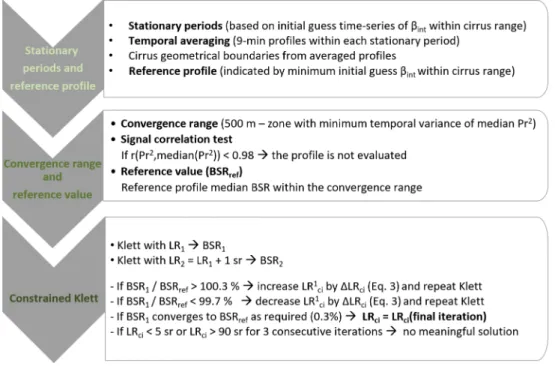
An extended method for cirrus optical retrievals is proposed, hereafter mentioned asconstrained Klett. A backward Klett–Fernald retrieval [63,64] was employed, constrained by the backscatter ratio (BSR), which is the ratio of molecular and particulate backscatter over molecular backscatter, beneath the cirrus cloud. TheLRciwas iteratively adjusted until the BSR matched with a reference BSR value (BSRref). The main steps of theconstrained Klettmethod are outlined in Fig.4. The constrained Klettalgorithm is given in Code 1 [53]. Theconstrained Klettmade use of the assumption that the aerosol content beneath the cirrus cloud was invariable. In order to enhance the validity of this assumption, the near-rangereference value(also called calibration value) was set within the range of minimumPr2signal variance (convergence range). Theconvergence rangewas bounded between the full overlap range (600 m) and 1 km beneath the minimumCbase. In this way, artificial signal gradients as well as cirrus adjacent areas, where turbulence and ice seeding are more likely, were avoided. Theconvergence rangewas a 500 m-zone, where the medianPr2signal presented minimum temporal variance. When the variance was equally low in more than one zones, the higher zone was selected, because the Klett errors increase with the integration from the far range. In order to further enhance the validity of aerosol content stability assumption, profiles not highly correlated with the temporal median profile (r<0.98) were discarded.
Fig. 4.Flowchart of configuration procedure (section2.3.1) and optical characterization (section2.3.2) withconstrained Klettmethod. Theconstrained Klettalgorithm is given in Code 1 [53].
An initial guess Klett–Fernald retrieval was first performed using two LR zones, one within the cirrus layer (assumedLR355ci =20 sr andLR532ci =28 sr) and one zone outside (assumedLR355
=35 sr andLR532=36 sr). TheLRcivalues were needed for initializing the Newton-Raphson method and they can be arbitrary provided that they are close enough to the unknown quantity [65]. Therefore, theLRciinitial values were selected close to those most frequently reported by other studies (e.g. [56,66–68]). Regarding the LR values outside the cirrus layer we used background values for the site of Ny-Ålesund based on statistics provided by Ritter et al. (2016) [69]. These LR values should be adapted accordingly for different lidar sites.
Subsequently, theβintwithin the cirrus range was estimated. Although theβintwas an initial guess, its minimum corresponded to low COD layers. The lower theβintthe lower the effect of a wrongly chosenLRcion the Klett solution. Therefore, thereference profilecorresponded to the profile of minimumβintor to a temporally close cloud-free profile (if available). TheBSRref was estimated from thereference profileas the median BSR within theconvergence range. In section 4.1we investigate the upper COD limit for deriving an accurateBSRref. The effect ofBSRref statistical uncertainties on the optical properties is also investigated (section4.2).
Once theconvergence range, thereference profileand theBSRref were defined, the recursive Klett procedure was initiated. Two initial guess Klett retrievals were performed, one withLR1ci and another withLR2ci=LR1ci+1 sr (see lower part of Fig.4). Upon each iteration, the median BSR within theconvergence rangewas estimated (BSR1andBSR2as derived from the retrieval withLR1ciandLR2ci, respectively). When the ratio of BSR1 over BSRref exceeded the desirable convergence percentage(set to 0.3% after sensitivity analysis, see section4.2), theLRciwas adjusted by a factor∆LRci(Eq. (3)). Following the Newton–Raphson method (described in Ryaben’kii and Tsynkov (2006) [65]), the∆LRcifactor was formulated as the difference ofBSRref andBSR1over the difference ofBSR1andBSR2, the latter being equivalent to∂BSR∂LR with dLR=1 sr.
∆LRci= BSRref −BSR1
BSR1−BSR2 (3)
The iterative process was bounded by physically meaningfulLRcivalues, i.e. between 5 sr and 90 sr. A wide range of boundingLRcivalues was employed as we did not want to a priori exclude physically possibleLRcivalues. The selection was based on previous experimental (at different locations) [40,70] and modeling studies [71–73]. For instance, Ansmann et al. (1992) [40]
reported values between 5-15 sr over a marine mid-latitude site, using the Raman technique. Chen et al. (2002) [70] reported over TaiwanLRcivalues lower than 10 sr in some cases. Okamoto et al. (2019) and (2020) [72,73] performed modeling simulations and reportedLRcivalues at 355 and 532 nm starting from approximately 5 sr and exceeding 100 sr for 2-D plates depending on the effective angle between the particle symmetrical axis and the laser beam (Fig. 5 from Okamoto et al. (2019) [72], Fig. 8 and Fig. 9 from Okamoto et al. (2020) [73]).
The retrieval was considered successful once theBSR1 solution matched with theBSRref. The resultingβpartand vertically-constantLRciwere used for estimating the COD according to Eq. (4):
COD=∫ Ctop Cbase
LRci·βpart(r)dr (4)
2.3.3. Existing optical retrievals: double-ended Klett and Raman
In order to gain confidence in the proposedconstrained Klettmethod, two established retrievals were also applied, namely the double-ended Klett and Raman [40]. Concerning the constrained Klett, different sets of backward and forward Klett–Fernald retrievals [63,64] were performed with changingLRcivalue. TheLRciresulting in the lowestroot mean square errorbetween the backward and forwardβpartprofiles was selected. TheLRciwas modified within physically expected values of 5 and 90 sr as in the constrained Klett [40,70–73]. In this work the
Fig. 5.Height-time plot of lidarPr2signal (a). Different symbols present theCbaseand Ctopresulting from dilation values between 30 and 120 m. Red vertical lines (panel a) denote the selected profiles ofPr2and WCT (presented in panels b and c). Higher inter-dilation spread was observed for smooth-shaped boundaries (b).
Klett–Fernald calibration window was set in the stratosphere for the backward retrieval and in theconvergence rangefor the forward retrieval. In this way, the retrieval was comparable to theconstrained Klett. However, it should be noted that the classical double-ended Klett method assumes zeroβpartbelow and above the cirrus cloud [40]. The impact of this aerosol-free assumption is investigated in section5.
The cirrus optical characterization and theBSRrefestimation was also performed via the Raman technique. This technique provides the backscatter and extinction coefficients independently [40] and, thereby, a vertically-dependentLRci can be derived. In this study, we report the vertically averaged Raman derived LRci to facilitate the comparison withconstrained Klett (section2.3). Theαpartat 355 and 532 nm is based on the rotational-vibrational Raman signals of 387 and 607 nm, respectively. Since the Raman cross-sections are orders of magnitude smaller than the elastic scattering cross-sections, the Raman technique is usually limited to night-time applications. In order to reduce the noise of the weak Raman signals, profiles were smoothed with a Savitzky–Golay filter [74]. The smoothing window was equal to one-third of the minimum cirrus cloud thickness. The molecular number density, which is needed for estimating theαpart, was derived by collocated radiosonde ascents from the AWIPEV research base. The Ångström
exponent of ice crystals for the wavelength pairs of 355-387 nm and 532-607 nm was assumed equal to unity. This is a reasonable assumption since the size of the ice crystals is usually sufficiently large compared to the ultraviolet and visible wavelengths [40]. Raman extinction uncertainties stem from statistical signal noise and uncertainties in molecular number density, which were, however, low within the cirrus layers. The comparison between theconstrained Klett, the double-ended Klett and Raman retrievals is presented in section5and their limitations and strengths are discussed in section6.
2.4. Multiple scattering correction
The effect of multiple scattering cannot be neglected when the size of the scatters is large compared to the emitted wavelength. The effect is more pronounced if the lidar system has a wide telescope FOV and a non-negligible laser beam divergence. The multiple scattering effect does not only depend on the COD but also on ice crystal effective radius (reff) and laser beam cloud penetration depth. For this reason, an analytical model is needed in order to correct for high order scattering events. In this study, we used the multiple scattering correction (MSC) model of Eloranta (1998) [75], which is openly available (http://lidar.ssec.wisc.edu/multiple_scatter/ms.htm). The Eloranta model assumes the presence of hexagonal ice crystals for phase function calculations. Moreover, a mono-disperse ice crystal vertical distribution was assumed. The ice crystalreff was estimated as a quadratic function of temperature, following the parameterization of Wang and Sassen (2002) [76] given by Eq. (5):
reff =90.14+0.659·T−0.004·T2 (5) The model simulates the ratio of up to seven-order(Ptot)to single scattering photon power (P1) as a function of range (r) and wavelength (λ). Sensitivity tests revealed that higher than three-order scattering events contributed negligibly to the total photon power. Therefore, the first four scattering orders were finally taken into account as a compromise between accuracy and computational speed. Initially, the apparentαpart, denoted asαapp(orβpartmultiplied by theLRci) was incorporated into the MSC model. Subsequently, a first estimation of the multiple scattering factor F(λ,r) (Eq. (6)) and the quasi-corrected extinction (α(λ,r)) (Eq. (7)) were obtained:
F(λ,r)=
d
drlnPPtot1(r)(r)
2·αapp(λ,r)+drd lnPPtot1(r)(r) (6)
α(λ,r)= αapp(λ,r)
1−F(λ,r) (7)
As a next step, the quasi-correctedα(λ,r)was incorporated again into the MSC model. This recursive procedure was repeated until the MSC model converged to a stable F(λ,r). Usually, only two iterations already provided sufficient convergence. A similar procedure was followed in previous studies [56,66,68]. A simplified MSC approach, which is only dependent on the COD was introduced by Platt (1973) [14] and is frequently used in literature ([42,70]). Eq. 8 describes the simple MSC factor n, with the MSC COD being the ratio of the apparent COD over the factor n. The analytical and simplified MSC approaches are compared in theAppendix.
n= COD
eCOD−1 (8)
3. Sensitivities on cirrus geometrical properties 3.1. Wavelet covariance transform - dilation sensitivity
Since the WCT dilation is an important parameter for accurate and precise cirrus detection (section 2.2), a relevant sensitivity analysis is performed here. Thanks to the high vertical
resolution (7.5 m) of KARL signals, we explored small dilation values between 30 m (4 range bins) and 120 m (16 range bins), presented with different symbols in Fig.5. After analyzing a significant number of cirrus layers, it was observed that dilation values smaller than 90 m were less sensitive to smooth-shaped cirrus layers, as shown in Fig.5(b) (smooth signal gradients close toCtop). On the contrary, the 90 m dilation was more effective for faint layers and efficiently captured layers thinner than 200 m layers, as for 7:30-9:00 UT on 23 January 2019 (Fig.5(a)).
Detecting faint layers near theCbaseis important, since the multiple scattering effect is higher there ([77] andAppendixof this study). Overall, the discrepancies arising from the dilation selection were low, with the majority of inter-dilation spread being lower than 50 m.
3.2. Wavelet covariance transform - wavelength dependency
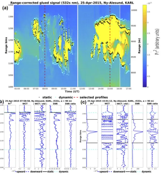
The dependency of cirrus detection on wavelength was assessed both by the dynamic and static WCT methods. Since the SNR depends on background illumination conditions, both daytime (25 April 2015, Fig.6(a)) and night-time (23 January 2019, Fig.6(b)) cirrus clouds were investigated. In Fig.6(a) and6(b) the dynamic (open symbols) and static (dot symbols) WCT derived boundaries are demonstrated for different wavelengths. Thin and faint cirrus layers were not so discernible in the 355 nm channel with parallel polarization (355p- cyan symbols) as in the other wavelengths due to the strong UV Rayleigh scattering (Fig.6(b), for example at 8:30–10:00 UT). This behavior was more profound for the static WCT method. Concerning the 355 nm channel with perpendicular polarization (355s- black symbols), this was strongly affected by noise during daytime (Fig.6(a)), with noise peaks frequently detected even with increasedSNR ratiothresholds. In the 532pchannel (green symbols) both the static and dynamic methods mostly detected the stronger cirrus parts (Fig.6(a), for example at 14:00–16:00 UT).
The cirrus layer presented in Fig.6(c) was characterized by smooth-shapedCbaseand strong- shapedCtop. Therefore, the discrepancies across different wavelengths were larger for theCbase. The static (dotted lines) and dynamic (dashed lines) WCT derived boundaries are given for the different channels. The 355pand 532pchannels detected mostly central cirrus parts. In contrast, the 355s, 532s(light green) and 1064 nm (red symbols) channels were more sensitive to faint marginal parts and showed better inter-agreement, especially for the dynamic method. Moreover, the SNR of the perpendicular polarization channels was higher compared to those with parallel polarization and theSNR532was higher thanSNR355. In general, longer wavelengths perform better in discriminating clouds from aerosol. However, the KARL system records 1064 nm signals in analog mode, which is more prone to noise.
For the aforementioned reasons, the 532schannel was finally selected for cirrus detection as the longest wavelength and highest quality available channel. It should be mentioned, however, that under specific conditions the 532sderived boundaries also presented variability. For instance, fluctuating geometrical boundaries can be seen at 8:00–10:00 UT (Fig. 6(b)) due to weak gradients, especially close to theCtop. Variability was also revealed during 13:00–14:00 UT (Fig.6(b)), with weak signal gradients overhead of strong ones. This variability was lower for temporally averaged signals thanks to higher SNR. The optimalSNR ratiothresholds for each channel of KARL are given in theAppendix.
3.3. Dynamic - static wavelet covariance transform comparison
In the following, thedynamic WCTmethod is compared to the static one. Both methods were applied on 532ssignals using a 90 m dilation. Two daytime cirrus layers (Fig.7(b) and7(c)), which were highly affected by background illumination, are analyzed in detail. The dynamic method was more sensitive to weak signal gradients that, however, exceeded the signal standard deviation. For instance, on 25 April 2015, 7:59 UT (Fig.7(b)), the cirrus layer presented -0.07
Fig. 6. Height-time plot of lidarPr2 signal for daytime (a) and night-time (b) cirrus clouds. Overlaid with different colors are the cirrus geometrical boundaries as derived by the dynamic (open markers) and static (dot markers) WCT method. Selected profiles ofPr2, WCT,
|︁
|︁
|︁
|︁
WCT/std
|︁
|︁
|︁
|︁, SNR andSNR ratioare presented together with the dynamic (dashed lines) and static (dotted lines) WCT derived boundaries (c). The 532schannel was finally selected for cirrus detection.
WCT and
|︁
|︁
|︁
|︁
WCT/std
|︁
|︁
|︁
|︁equal to 3 at theCbase. Therefore, theCbaseof this cirrus layer was not detectable with the static method (0.3 WCT threshold, see [61]).
Fig. 7.Height-time plot of lidarPr2signal with overlaid dynamic (cyan) and static (black) WCT derived cirrus boundaries. Signal normalization accounts for background color changes (see section2.2). Selected profiles are denoted with red vertical lines (a) and presented in panels (b) and (c), where horizontal lines indicate the dynamic and static cirrus boundaries.
Solid (dashed) blue lines correspond to upward (downward) profiles used forCbase(Ctop) detection. Thedynamic WCTwas more sensitive to faint and marginal parts of cirrus layers.
Another strength of the dynamic method lies on its increased sensitivity to marginal cirrus layers. On 25 April 2015, 15:01 UT (Fig.7(b)), the static method was only sensitive to stronger cirrus parts, while the dynamic method detected theCbase(Ctop) 277.5 m (285 m) out of the static-derived boundaries. Hence, the cirrus geometrical thickness was underestimated by more than 500 m by the static method. Increased sensitivity to cirrus marginal layers is also an important advancement of the latest CALIOP CAD algorithm. More details will be discussed in section6. It should be mentioned that sometimes both the dynamic and static WCT methods
failed to detect the cirrus boundaries, especially for faint cirrus layers, as for 8:00–9:00 UT on 25 April 2015 (Fig.7(a)). Overall, the dynamic method detected faint cirrus layers that otherwise could not have been detected by the static method.
4. Accuracy and uncertainty assessment 4.1. Reference value accuracy and limitations
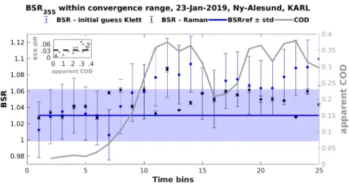
The cirrus cloud of 23 January 2019 was selected for assessing the accuracy and inherent uncertainties ofconstrained Klett, since it comprised different regimes from sub-visible to lower opaque layers [42]. Concerning thereference value(see section2.3.2), this was calculated from a cloud-free profile (BSRcloud−freeref ) observed at 7:47-7:56 UT prior to the cirrus cloud passing over Ny-Ålesund. Theconvergence range(see section2.3.2) was selected at 5.5– 6 km, where the signal temporal variance was minimum. TheBSRref accuracy was evaluated by estimating the same quantity via the Raman technique (BSRRamanref ). This analysis is illustrated in Fig.8.
The blue line and shaded area (median±standard deviation) denote theBSRcloud−freeref , while the BSRRamanref (black symbols) andBSRguessref (blue symbols) are also presented.
Fig. 8. BSR355within theconvergence range(median±standard deviation) as derived by the initial guess Klett (BSRguessref , blue symbols) and Raman retrievals (BSRRamanref , black symbols). BSRRamanref errorbars are smaller due to a 75 m-smoothing of the BSR profile.
For comparison, a preceding cloud-free profile provided theBSRcloudref −free(blue line and shaded area denote its median±standard deviation). The apparent COD is given on the right axis. The difference betweenBSRguess
ref andBSRcloud−free
ref versus the apparent COD are presented in the upper left inset figure. A sufficiently accurateBSRguessref can be obtained from cirrus layers with 0.2 maximum COD. TheBSRguessref mostly agrees withBSRRamanref within the range of uncertainties.
At 355 nm (532 nm, not shown) the initial guess Klett provided a median±standard deviation BSRcloud−freeref of 1.03±0.03 (1.07±0.02), while the Raman yieldedBSRRamanref equal to 1.06±0.01 (1.06±0.02).BSRcloud−freeref andBSRRamanref were in agreement within the range of uncertainties, this being satisfactory, taking into account the high Raman statistical uncertainties especially for fine temporal scales (here 9 min). Thus, theBSRref parameter was estimated with sufficient accuracy.
If cloud-free profiles were not available, the minimumβint(or COD) profile would have been selected asreference profile(see section2.3.2). However, in such cases theBSRref accuracy would have been subject to an upper COD limitation. More specifically, the lower the cirrus COD the more accurate is theBSRguessref expected to be, with the impact of a wrongly assumed LRcion the initial guess Klett being lower. In order to quantitatively assess the effect of COD on theBSRguessref accuracy, we compared theBSRguessref withBSRRamanref for every single profile of the 23 January 2019 cirrus. Then, we assessed up to which COD theBSRguessref accuracy is acceptable.
As it can be seen, a sufficiently accurateBSRguess
ref can be obtained for COD up to 0.2 (Fig.8, right axis). This is illustrated more clearly on the upper left inset figure, with theBSRguessref lying within theBSRcloud−freeref uncertainty (dashed line) for 0.2 maximum COD. Hence, even if the minimum COD profile (here time bin 1) was selected instead of a cloud-free profile, the resultingBSRguessref would have agreed with theBSRcloud−freeref andBSRRamanref .
Another significant remark concerns the aerosol content stability beneath the cirrus cloud, which is assumed both by the constrained and double-ended Klett retrievals. As displayed in Fig.8, theBSRRamanref variability lied within the uncertainty of theBSRcloud−freeref reference value, indicating that the stability assumption was valid. Finally, it should be underlined that the upper COD limitation discussed above only concerns thereference profile selection. As long as a sufficiently accurateBSRref is obtained, theconstrained Klettcan be applied on any cirrus cloud regime.
4.2. Inherent uncertainties of constrained Klett
In order to assess the inherent uncertainties, we investigated the response of cirrus optical properties to the parameters of theconstrained Klettmethod, namely theconvergence percentage andreference value BSRref (see section2.3.2). In the first sensitivity analysis (Fig.9(a)) the convergence percentagewas modified between 0.1% and 0.5%, with 0.3% being the default. The LRciof optically thinner layers was more sensitive (maximum spread 10% or 3 sr) compared to thicker layers (maximum spread 5%). Overall, the COD was modified by less than 0.004 (1-10%
spread depending on the COD). Less strictconvergence percentages (higher than 1%, not shown) were incapable of constraining theLRciwith acceptable accuracy.
The impact ofBSRref statistical uncertainties on the optical properties was also evaluated (Fig.9(b)). In the control case, the median value (BSRref=1.03) was used, while in the perturbed cases theBSRref was increased by 0.01 (blue symbols), 0.02 (grey symbols) and 0.03 (cyan symbols). These uncertainties were typically encountered during the analysis of different cirrus clouds (2011-2020) over Ny-Ålesund, Svalbard. Low COD layers (corresponding to time bins 1–5) were more sensitive to theBSRref parameter. More specifically, if theBSRrefwas perturbed too far from the control case, reasonable results were not always possible to obtain. Therefore, an accurateBSRguessref is crucial. TheLRcidisplayed higher sensitivity for optically thinner layers (14–19 sr or 74 and 60% with respect to control values of 19 sr and 32 sr). Lower sensitivity (less than 3 sr or 13% with respect to control value of 24 sr) was found for opaque layers. The COD sensitivity was higher for lower optically-thin and opaque regimes, varying between 0.02 and 0.03 (7-50% with respect to control values of 0.3 and 0.06) for the most perturbed case.
4.3. Effect of geometrical boundaries on the optical properties
In the following we assess the effect of cirrus detection method on the apparent optical properties.
To this end, the cirrus geometrical properties were determined via the dynamic (Fig.10(a), cyan symbols) and static WCT methods (black symbols). Based on the dynamic and static derived boundaries, we retrieved the optical properties via theconstrained Klettand investigated the resulting discrepancies (Fig.10(b)). The optical discrepancies are illustrated as a function of
Fig. 9.Sensitivity of optical properties with respect to theconvergence percentage(a) and thereference value(BSRref, b) parameters of theconstrained Klett. Absolute differences with respect to the control case are presented with open symbols on the right axis. Dashed horizontal lines denote the optically-thin and sub-visible COD regimes according to [42].
Optically thinner layers displayed higher sensitivity, especially with respect to theBSRref parameter.
geometrical discrepancies (symbol size). As geometrical discrepancies we defined the cumulative difference ofCbaseandCtopbetween the static and dynamic method.
Fig. 10.Height-time plot of temporally averagedPr2signal with overlaid dynamic (cyan) and static (black) WCT cirrus boundaries (a). Corresponding optical properties as derived by theconstrained Klettmethod (b) and differences (blue dots) as a function of the geometrical discrepancy (dot size). The geometrical discrepancies varied from 30 to 1613 m. Optically thinner layers were affected more intensely.
Higher geometrical discrepancies mostly occurred for faint cirrus layers (Fig.10(a)). The dynamic method provided higher COD values, since thanks to its higher sensitivity, it usually yielded wider boundaries. Higher optical discrepancies arose for upper sub-visible and optically thin layers. The highestLRciand COD differences (45% or 17 sr and 93% or 0.037, respectively) were related to the maximum geometrical discrepancy (1613 m). The geometrical discrepancy, however, was a necessary but not sufficient condition for optical discrepancies to occur. More specifically, in opaque layers despite the non-negligible geometrical discrepancy (up to 490 m), theLRciand COD solution discrepancies were low (less than 1 sr and 0.025, respectively).
This indicates that the solution converges faster within the main part of optically thicker layers
thanks to sufficient light attenuation and, thus, marginal parts play a less critical role. Overall, for optically thin and opaque layers theLRcidifference was lower than 10% (3 sr) and the COD difference did not exceed 8% (0.025). Finally, one should bear in mind that the MSC optical discrepancies are expected to be higher than the apparent ones, which were presented here. The same sensitivity is performed on the double-ended Klett and Raman derived optical properties in theAppendix.
5. Inter-comparison of cirrus optical properties
The comparison ofconstrained Klettderived optical properties with those from the double-ended Klett and Raman retrievals is shown for the cirrus cloud of 23 January 2019. Thedynamic WCT method provided theCbaseat 7±0.2 km andCtopat 8.8±0.2 km, with the ambient temperature at -48 and -63oC, respectively. The MSCLR355ci andCOD355as derived from the different retrievals are presented in Fig.11. More details on the multiple scattering effect are given in theAppendix.
Fig. 11.Inter-comparison ofconstrained Klett, double-ended Klett and Raman retrievals in terms of MSC optical properties at 355 nm (mean±standard deviation given in the legend). For Klett retrievals, errorbars represent uncertainties due to 0.01 BSRreference valueerror. For the Raman method,LRcierrorbars represent the standard error of the mean (extremely high for vertically inhomogeneous layers), while COD errorbars represent the integral-propagatedαpartuncertainty.
The double-ended andconstrained Klettexhibited high agreement, especially in the COD. The Raman technique provided lower vertically-averagedLRciand COD solutions, probably because of the vertical smoothing process. HigherLRcidiscrepancies occurred for layers with COD lower than 0.1. This could be attributed to less efficient convergence of theconstrained Klettas well as to higher Raman statistical uncertainties. The mean (±standard deviation) discrepancy between constrained and double-ended Klett amounted to 3±4 sr forLR355ci (1±2 sr forLR532ci ) and 0.01±0.007 forCOD355(0.02±0.02 forCOD532). The corresponding discrepancies between constrained Klettand Raman were equal to 10±6 sr forLR355ci (14±12 sr forLR532ci ) and 0.07± 0.04 forCOD355(0.06±0.06 forCOD532). Overall, the three retrievals exhibited agreement within the range of uncertainties on the mean cloud optical properties. TheCOD355(LR355ci ) was estimated 0.28±0.17 (29±4 sr) by theconstrained Klett, 0.27±0.15 (32±4 sr) by the
double-ended Klett and 0.22±0.12 (26±11 sr) by the Raman retrievals. Similar agreement was found for the optical properties at 532 nm (not shown). The optical properties are comparable to those derived, via double-ended Klett and Raman retrievals, over the sub-Arctic site of Kuopio (62.7oN) withCOD355of 0.25±0.2 andLR355ci of 33±7 sr [56].
The high agreement between the double-ended andconstrained Klettretrievals can be attributed to the fact that both rely on elastic signals. There is an additional reason, however, behind this agreement. In this study, we used identical far- and near-rangereference valuesfor both methods in order to make them as comparable as possible. Nevertheless, we should underline that the classical double-ended Klett is based on aerosol-free assumptions above and below the cirrus cloud [40]. Therefore, we performed a sensitivity analysis to assess the impact of the latter assumption. In Fig.12, theLRciand COD are presented as in Fig.11but the double-ended Klett with aerosol-free assumptions (BSR=1) is additionally given. As revealed, optically thinner layers (time bins 1 to 5) were the most affected ones by the aerosol-free assumption, displaying LRciof 75±7 sr (mean±standard deviation). Previously, theLRciwas assessed at 31±2 sr by the double-ended Klett, 24±5 sr by theconstrained Klettand 38±5 sr by the Raman retrieval. For optically thicker layers the aerosol-free assumption led to positive discrepancies (2–8 sr) as well, while the overall COD discrepancies lay between 0.01 and 0.03. Hence, theLRci was overestimated since the amount of extinction that was overlooked due to the aerosol-free assumption was instead attributed to the cirrus layers. Consequently, a non-realisticBSRref assumption can make a fundamental difference in the solution accuracy.
Fig. 12.Same as Fig.11except for apparent optical properties and additional double-ended Klett with aerosol-free assumptions (BSR=1). Non-realisticreference valuescan introduce biases in the optical properties, especially for optically thinner layers (44 sr averageLRci bias).
Theconstrained Klettmethod was applied to a large number of cirrus layers with variable vertical structure, geometrical and optical thickness observed at different altitudes both during day-time and night-time. TheLRciand COD distributions as obtained from the three different retrievals, i.e.constrained Klett, double-ended Klett and Raman (when applicable) presented high similarities both at 355 and 532 nm. Moreover, it was found thatLRciclose to the bounding values (5 and 90 sr) were associated with cirrus layers of low geometrical depth and COD. For these regimes cirrus detection and optical characterization is more challenging (section3.3,4.2, 4.3andAppendix) and therefore care will be taken when providing long-term cirrus properties statistics (e.g. exclude cirrus layers with COD lower than 0.02).
6. Discussion
6.1. Limitations of existing cirrus cloud retrievals
The limitations of cirrus optical retrievals already existing in literature are briefly discussed here.
Starting with the transmittance method, it relies on the ratio of backscattering signals atCbaseand Ctop, which is quadratively proportional to the cirrus layer transmission [37–39]. However, the transmittance method cannot converge adequately for optically thinner cirrus (COD below 0.05) [70]. Concerning the backward - total optical depth method [41], this derives an initial guess COD via the slope method. Then, anαpartprofile is obtained by a backward or forward Klett and, finally, it is modified to match with the initial guess COD. Nevertheless, the slope method requires negligible molecular extinction and backscatter contribution within the cloud, clear air atCbaseandCtopand negligible multiple scattering effect. Therefore, no reasonable accuracy can be achieved either for optically thinner cirrus (COD below 0.1) or in the presence of overhead aerosol layers. Finally, the Raman technique [40] is typically limited to night-time applications because it relies on the weak Raman signals (section2.3.3). Therefore, Raman signals are usually smoothed vertically at the expense of effective resolution [78] and clustered over long temporal periods. However, distortedαpart profiles might be produced, with ice crystal related peaks being suppressed, having a critical impact on the accuracy of radiative effect estimates [23].
Exemplarily, vertical smoothing of 780 m can lead to biases of 64% (7.7Wm−2) at surface and 39% (11.8Wm−2) at top of the atmosphere for opaque cirrus layers [23]. Likewise long temporal averaging that smears out the cirrus physical variability, is expected to induce radiative effect biases. Therefore, an application of high-resolution daytime profiling, an approach developed for Raman lidar (as in [79]) is in our upcoming research interests.
6.2. Strengths and limitations of extended cirrus cloud retrieval
Cirrus detection and optical characterization is, in general, more challenging for geometrically and optically thinner cirrus layers. However, the proposeddynamic WCTmethod proved to be more sensitive to faint cirrus layers that were partly or completely overlooked by the static method (section3.3). A similar advancement has been achieved in the 4th version of CALIOP CAD algorithm [31], which shows increased sensitivity to optically thinner layers adjacent to cirrus clouds (cirrus fringes). At the same time, however, miss-classification into aerosol increased slightly, as a side effect of higher calibration accuracy and increased sensitivity to high altitude depolarizing aerosol. Consequently, there is still place for improvement in the CALIOP CAD algorithm. The optical biases, which result from cirrus boundary miss-determination and can be relatively high for optically thinner layers (section4.3andAppendix), render CAD optimization crucial. To this end, the satellite-derived cirrus geometrical properties can be evaluated by ground-based lidar observations and, thereby, the CAD thresholds might be improved. Added value can be brought by ground-based lidar observations in the Arctic, where miss-classification issues are frequently reported [31–33].
Thedynamic WCTmethod enables the investigation of optically thinner layers (section3.3) that are, however, characterized by higher inherent uncertainties (section4.2) and more challenging LRcivalue adjustment process(section2.3.2). From a numerical viewpoint, theconstrained Klett cannot always provide a robustLRcivalue for low COD layers. The light attenuation within such layers is not sufficiently strong to scale the solution and appoint the best match.
Likewise the double-ended Klett solutions exhibit lower absolute differences and, hence, the best matching solution is more challenging to find. Based on our analysis, theconstrained Klettadjusts effectively theLRcifor apparent COD as low as 0.02 for both 355 and 532 nm. Comparable minimum COD values were reported over the sub-Arctic site of Kuopio (COD355=0.24±0.21 andCOD532 =0.22±0.2 [56]). In this respect, theconstrained Klettis expected to be more
robust for mid-latitude and tropical cirrus (accompanied by cloud-free profiles to ensure an accurateBSRref), the majority of which fall into the optically thin regime [55,66–68].
In this study, we demonstrated that highly accurate optical properties can be derived solely by a stable backward Klett retrieval, as long as an additionalreference valueis appointed beneath the cirrus cloud. More importantly, the near-rangereference valueis not simply assumed but approximated by an initial guess BSR value (BSRguessref ). This is a step towards more accurate retrievals, as this initial guess proved to agree with independent Raman estimates (section4.1), as long as low COD (below 0.2)reference profiles are selected. This upper COD limitation was only encountered in a minority of the analyzed cases over Ny-Ålesund (2011-2020). Even for mid-latitude and tropical cirrus, this limitation is nearly raised as the majority of these clouds mostly belong to the optically thin regime [55,66–68]. It should also be pointed out that our system KARL is not in24/7operation and, thus, cirrus clouds were neither monitored from their formation nor clear-sky observations prior to the cirrus passing were always available. However, for continuously operating lidar systems as those of the Micro-Pulse Lidar Network (MPLNET) [80] the maximum COD limitation can be lifted more easily.
One can benefit from the highly accurate near-rangereference valueproposed here, even if the double-ended Klett is applied. As demonstrated in section5, the double-ended Klett aerosol-free assumption can lead toLRci positive biases (Fig.12), especially in optically thinner layers.
Further limitations of theconstrained Klettrelate to the assumed as vertically-independentLRci. However, this is a common limitation in existing methods such as the transmittance, double-ended Klett and backward - total optical depth. Finally, the aerosol content stability assumption beneath the cirrus cloud proved valid (Fig.8) according to independent Raman estimates.
7. Summary and outlook
In this study, we explored the limitations and strengths of an extended cirrus cloud retrieval scheme. The scheme is based on lidar observations and comprises newly proposed cirrus detection (dynamic WCT) and optical characterization (constrained Klett). Cirrus clouds observed over the Arctic research site of Ny-Ålesund, Svalbard, were used for evaluating its performance. The WCT method (section2.2) [54], which is sensitive to signal gradients, was revised forCbaseand Ctopdetection. For the first time, twodynamic WCTcriteria were introduced (section2.2.1).
The first one was related to the ratio of WCT over the signal standard deviation (
|︁
|︁
|︁
|︁
WCT/std
|︁
|︁
|︁
|︁).
The second criterion compared the SNR in marginal cirrus areas to the SNR of adjacent areas (SNR ratio). Cirrus optical properties were derived by a newly introduced iterative Klett–Fernald method [63,64], calledconstrained Klett(section2.3.2). The novelty ofconstrained Klettis the recursively determinedLRcithat was constrained by an additionalreference value(BSRref) beneath the cirrus cloud. TheBSRrefwas estimated either from cloud-free profiles or profiles with minimum cirrus influence (COD up to 0.2). The main findings of this study can be summarized as follows:
• Increased sensitivity to thin cirrus layers (less than 200 m) was achieved thanks to the dynamic WCTmethod and the high vertical resolution (7.5 m) of KARL signals. The dynamic WCTmethod was more sensitive to faint layers, which were, in some cases, partly or completely missed by the static method (section3). Fine-scale temporal averaging (9 min) was only performed within periods of physical stationarity to obtain non-distorted profiles (section2.3.1).
• Theconstrained Klettwas applicable to all cirrus regimes for COD values down to 0.02.
Thereference value(BSRref) was highly accurate, since it agreed with independent Raman estimates. Even without cloud-free reference profiles, accurateBSRref estimates were obtained from layers with COD up to 0.2 (section4.1).