Quantum Spin Liquids

Quantum Spin Liquids

David Urwyler

Condensed Ma2er Physics (PHY 401)

Ferro-/Antiferromagnetic materials

• Heisenberg Model: 𝐻 = − 𝐽 ∑ 𝑆

' 𝑆

𝐽 > 0 → Ferromagnet

𝑇 < 𝑇_!

𝐽 < 0 → An4ferromagnet

𝑇 < 𝑇_"

Frustrated magnets

Example:

• An4ferromagnet

• NN-interac@on

• Localized spins

• Exchange interac4on that cannot be simultaneously sa4sfied

?

Geometrical origin of frustra4on

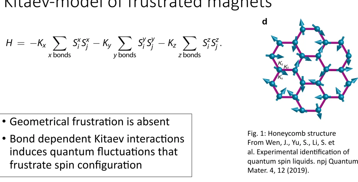
Kitaev-model of frustrated magnets

• Geometrical frustra4on is absent

• Bond dependent Kitaev interac4ons induces quantum fluctua4ons that frustrate spin configura4on

field. This model, as in Eq. 1, is named the Kitaev model.

H ¼ "K_x X

xbonds

S^x_i S^x_j "K_y X

ybonds

S^y_i S^y_j "K_z X

zbonds

S^z_iS^z_j: (1)

Here, H is the Hamiltonian and K_x,y,z are the nearest-neighbour Ising- type spin interactions along the x, y andz bonds (Kitaev interactions).

It has been shown that the exact ground state of the Kitaev model is a QSL, which may be gapped or gapless depending on the relative strength of the Kitaev interactions along the three bonds.¹³ Unlike QSLs described by the RVB model, the QSL state in the Kitaev model (Kitaev QSL hereafter) is defined on the honeycomb lattice where geometrical frustration is absent. Instead, the presence of bond- dependent Kitaev interactions induces strong quantum fluctuations that frustrate spin configurations on a single site, resulting in a Kitaev QSL state.

The Kitaev model is simple and beautiful but was considered as a ‘toy’ model in the beginning, since the underlying anisotropic Kitaev interactions are unrealistic for a spin-only system. One brilliant proposal to realize the Kitaev interaction is to include the orbital degree of freedom in a Mott insulator that arises from the combination of the crystal electric field, spin–orbital coupling (SOC), and electron correlation effects.¹⁴ A Mott insulator is an insulator that band theory predicts to be metallic, but turns out to be insulating due to electron–electron interactions.¹⁵ In the proposal,¹⁴ the electronic configuration is a consequence of the following processes: First, the octahedral crystal field splits the d orbitals into triply degenerate t_2g and doubly degenerate e_g orbitals at low and high energies, respectively; second, in the presence of strong SOC, the degeneracy of the t_2g is lifted, giving rise to one effective spin J_eff=1/2 and one J_eff=3/2 band, both of which are entanglements of the S=1/2 spin and L_eff=−1 orbital moment for t_2g; third, the resulting J_eff=1/2 band is narrower than the original triply degenerate t_2g band. Consequently, a moderate electron correlation will open a gap and split this band into a lower and upper Hubbard band. Such a state is a J_eff=1/2 Mott insulator. Due to the spatial anisotropy of the d orbitals and strong SOC, the exchange couplings between the effective spins are intrinsically anisotropic and bond dependent, and will give rise to the Kitaev interactions under certain circumstance.^13,14 These advancements bring the hope to find Kitaev QSLs in real materials, and have motivated intensive research in searching for QSLs beyond the triangular, kagome and pyrochlore lattices in recent years.^16,17

WHY QSLS ARE OF INTEREST

QSL is a highly nontrivial state of matter. Ordinary states are often understood within Landau’s framework in terms of order, phase transition and symmetry breaking. However, a QSL does not have a local order parameter and avoids any spontaneous symmetry breaking even in the zero-temperature limit, so to understand it requires theories beyond Landau’s phase transition theory. In fact,

?

?

J a

K K K

d c

b

Fig. 1 Schematics of some typical two-dimensional crystal structures on which quantum spin liquids may be realized. a, b Triangular, c Kagome, and d Honeycomb structures. Arrows and question marks represent spins and undetermined spin configurations due to geometrical frustration, respectively.Jis the Heisenberg exchange interaction, and K_x,y,z are Kitaev interactions along three bonds. The shades illustrate spin singlets with a total spin S=0, each formed by two spins antiparrallel to each other

Table 1. Geometrically frustrated quantum-spin-liquid candidates

Material Structure Θcw (K) J (K) Reference

κ-(BEDT- TTF)2Cu2(CN)3

Triangular −375 250 ⁸⁴

EtMe3

Sb[Pd(dmit)2]2

Triangular −(375−330) 220–250 ⁸⁵

YbMgGaO4 Triangular −4 1.5 ³²

1T-TaS2 Triangular −2.1 0.1 ⁸⁶

ZnCu3(OH)6Cl2

(herbertsmithite) Kagome −314 170 ⁸⁷

Cu3Zn(OH)6FBr

(barlowite) Kagome −200 170 ⁸⁸

Na4Ir3O8 Hyperkagome −650 430 ²⁷

PbCuTe2O6 Hyperkagome −22 15 ²⁸

Ca10Cr7O28 Distorted kagome −9 ³⁴

Θcw and J are the Curie–Weiss temperature and exchange coupling constant, respectively

*Notes:

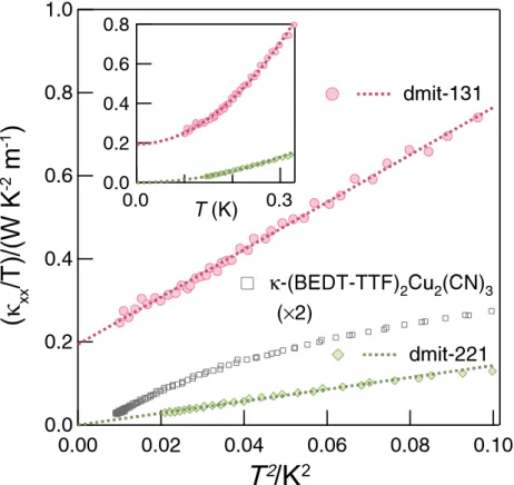
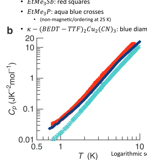
κ-(BEDT-TTF)₂Cu₂(CN)₃: With a J~ 250 K, no magnetic order nor spin freezing is observed down to 20 mK,⁸⁹ giving rise to a frustration index over 10,000. While low-temperature specific heat measurements indicate the presence of gapless magnetic excitations,⁶² they do not contribute to the thermal conductivity⁶³

YbMgGaO₄: A frequency-dependent peak in the a.c. susceptibility characteristic of a spin glass is observed around 0.1 K³³

1T-TaS₂: Note thatΘcw andJlisted in the table are significantly smaller than those calculated from the high-temperature susceptibility in ref. ³⁵ In 1T- TaS₂, 13 Ta⁴⁺ ions form a hexagonal David star cluster when the system is cooled below the commensurate charge density wave phase transition temperature at 180 K.⁹⁰ Twelve Ta⁴⁺ ions in the corner of the star form six covalent bonds and the spins connected by the bonds cancel out. An orphan electron is localized in the centre of the David star, giving rise to a net spin ofS=1/2 for each David star. The spins in the centre constitute a triangular network, making the system essentially a geometrically frustrated magnet. At present, whether or not this material is a QSL is still under hot debate^{35,86,90–92}

Na₄Ir₃O₈: Although a well-defined magnetic phase transition is not observed in Na₄Ir₃O₈, a spin-glass transition occurs around 6 K, below which the spins are frozen and maintain short-range correlations^27,93,94 Ca₁₀Cr₇O₂₈: It is a system with complex structure, and more interestingly, with dominant ferromagnetic interactions.³⁴ Frequency-dependent peak was observed in the a.c. susceptibility, suggestive of a spin-glass ground state, but it is suggested that such a state could be ruled out by performing the Cole–Cole analysis on the a.c. susceptibility data.³⁴

J. Wen et al.

2

npj Quantum Materials (2019) 12 Published in partnership with Nanjing University

1234567890():,;

field. This model, as in Eq. 1, is named the Kitaev model.

H ¼ "K_x X

x bonds

S^x_i S^x_j " K_y X

ybonds

S^y_i S^y_j " K_z X

zbonds

S^z_i S^z_j : (1)

Here, H is the Hamiltonian and K_x,y,z are the nearest-neighbour Ising- type spin interactions along the x, y and z bonds (Kitaev interactions).

It has been shown that the exact ground state of the Kitaev model is a QSL, which may be gapped or gapless depending on the relative strength of the Kitaev interactions along the three bonds.¹³ Unlike QSLs described by the RVB model, the QSL state in the Kitaev model (Kitaev QSL hereafter) is defined on the honeycomb lattice where geometrical frustration is absent. Instead, the presence of bond- dependent Kitaev interactions induces strong quantum fluctuations that frustrate spin configurations on a single site, resulting in a Kitaev QSL state.

The Kitaev model is simple and beautiful but was considered as a ‘toy’ model in the beginning, since the underlying anisotropic Kitaev interactions are unrealistic for a spin-only system. One brilliant proposal to realize the Kitaev interaction is to include the orbital degree of freedom in a Mott insulator that arises from the combination of the crystal electric field, spin–orbital coupling (SOC), and electron correlation effects.¹⁴ A Mott insulator is an insulator that band theory predicts to be metallic, but turns out to be insulating due to electron–electron interactions.¹⁵ In the proposal,¹⁴ the electronic configuration is a consequence of the following processes: First, the octahedral crystal field splits the d orbitals into triply degenerate t_2g and doubly degenerate e_g orbitals at low and high energies, respectively; second, in the presence of strong SOC, the degeneracy of the t_2g is lifted, giving rise to one effective spin J_eff = 1/2 and one J_eff = 3/2 band, both of which are entanglements of the S = 1/2 spin and L_eff = −1 orbital moment for t_2g; third, the resulting J_eff = 1/2 band is narrower than the original triply degenerate t_2g band. Consequently, a moderate electron correlation will open a gap and split this band into a lower and upper Hubbard band. Such a state is a J_eff = 1/2 Mott insulator. Due to the spatial anisotropy of the d orbitals and strong SOC, the exchange couplings between the effective spins are intrinsically anisotropic and bond dependent, and will give rise to the Kitaev interactions under certain circumstance.^13,14 These advancements bring the hope to find Kitaev QSLs in real materials, and have motivated intensive research in searching for QSLs beyond the triangular, kagome and pyrochlore lattices in recent years.^16,17

WHY QSLS ARE OF INTEREST

QSL is a highly nontrivial state of matter. Ordinary states are often understood within Landau’s framework in terms of order, phase transition and symmetry breaking. However, a QSL does not have a local order parameter and avoids any spontaneous symmetry breaking even in the zero-temperature limit, so to understand it requires theories beyond Landau’s phase transition theory. In fact,

?

?

J

a

K K K

d c

b

Fig. 1 Schematics of some typical two-dimensional crystal structures on which quantum spin liquids may be realized. a, b Triangular, c Kagome, and d Honeycomb structures. Arrows and question marks represent spins and undetermined spin configurations due to geometrical frustration, respectively. J is the Heisenberg exchange interaction, and K_x,y,z are Kitaev interactions along three bonds. The shades illustrate spin singlets with a total spin S = 0, each formed by two spins antiparrallel to each other

Table 1. Geometrically frustrated quantum-spin-liquid candidates

Material Structure Θcw (K) J (K) Reference

κ-(BEDT-

TTF)₂Cu₂(CN)₃ Triangular −375 250 ⁸⁴

EtMe₃

Sb[Pd(dmit)₂]₂ Triangular −(375−330) 220–250 ⁸⁵

YbMgGaO₄ Triangular −4 1.5 ³²

1T-TaS₂ Triangular −2.1 0.1 ⁸⁶

ZnCu₃(OH)₆Cl₂

(herbertsmithite) Kagome −314 170 ⁸⁷

Cu₃Zn(OH)₆FBr

(barlowite) Kagome −200 170 ⁸⁸

Na₄Ir₃O₈ Hyperkagome −650 430 ²⁷

PbCuTe₂O₆ Hyperkagome −22 15 ²⁸

Ca₁₀Cr₇O₂₈ Distorted kagome −9 ³⁴

Θ^cw and J are the Curie–Weiss temperature and exchange coupling constant, respectively

*Notes:

κ-(BEDT-TTF)₂Cu₂(CN)₃: With a J ~ 250 K, no magnetic order nor spin freezing is observed down to 20 mK,⁸⁹ giving rise to a frustration index over 10,000. While low-temperature specific heat measurements indicate the presence of gapless magnetic excitations,⁶² they do not contribute to the thermal conductivity⁶³

YbMgGaO₄: A frequency-dependent peak in the a.c. susceptibility characteristic of a spin glass is observed around 0.1 K³³

1T-TaS₂: Note that Θcw and J listed in the table are significantly smaller than those calculated from the high-temperature susceptibility in ref. ³⁵ In 1T- TaS₂, 13 Ta⁴⁺ ions form a hexagonal David star cluster when the system is cooled below the commensurate charge density wave phase transition temperature at 180 K.⁹⁰ Twelve Ta⁴⁺ ions in the corner of the star form six covalent bonds and the spins connected by the bonds cancel out. An orphan electron is localized in the centre of the David star, giving rise to a net spin of S= 1/2 for each David star. The spins in the centre constitute a triangular network, making the system essentially a geometrically frustrated magnet. At present, whether or not this material is a QSL is still under hot debate^{35,86,90–92}

Na₄Ir₃O₈: Although a well-defined magnetic phase transition is not observed in Na₄Ir₃O₈, a spin-glass transition occurs around 6 K, below which the spins are frozen and maintain short-range correlations^27,93,94 Ca₁₀Cr₇O₂₈: It is a system with complex structure, and more interestingly, with dominant ferromagnetic interactions.³⁴ Frequency-dependent peak was observed in the a.c. susceptibility, suggestive of a spin-glass ground state, but it is suggested that such a state could be ruled out by performing the Cole–Cole analysis on the a.c. susceptibility data.³⁴

J. Wen et al.

2

npj Quantum Materials (2019) 12 Published in partnership with Nanjing University

1234567890():,;

Fig. 1: Honeycomb structure From Wen, J., Yu, S., Li, S. et al. Experimental idenAficaAon of quantum spin liquids. npj Quantum Mater. 4, 12 (2019).

Large degeneracy of the ground state (key property)

They also identified deviations from the Arrhenius form at lower tem- peratures as a result of Coulomb interactions between monopoles. In an intriguing paper, Bramwell and colleagues applied an old theory put forward by Onsager¹⁸ for the electric-field dependence of thermal charge dissociation in electrolytes — the Wien effect — to the magnetic analogue in spin ice, that is, to the dis association of monopole–antimonopole pairs with a magnetic field¹⁹. The theory allows an extraction of the absolute value of the magnetic charge of a monopole from the dependence of the magnetic relaxation rate on the magnetic field. The authors measured muon spin relaxation in Dy2Ti2O7 to obtain the rate, and from this they extracted a magnetic charge in near perfect agreement with theoreti cal expectations. In addition to these quantitative measures of the energy and charge of a monopole, two recent papers presented neutron-scat- tering mea surements in magnetic fields, interpreting them as evidence of monopoles and the ‘strings’ emanating from monopoles^20,21. Many more experiments in which the monopoles in spin ice are studied and manipulated are likely to emerge soon.

Quantum spin liquids

In spin ice, as the temperature is lowered, the spins themselves fluctuate ever more slowly, eventually falling out of equilibrium and freezing below about 0.5 K (from theory, it is predicted that, in equilibrium, the spins should order at T = 0.1−0.2 K (ref. 6)). This is a consequence of the large energy barriers between different ice-rule configurations, which require the flipping of at least six spins, and the weak quantum amplitude for such large spins to cooperatively tunnel through these barriers. By contrast, for materials with spins of S = ½ and approximate Heisenberg symmetry, quantum effects are strong, and there are no obvious energy barriers. I now turn to such materials in the search for a QSL ground state, in which spins continue to fluctuate and evade order even at T = 0 K. Such a QSL is a strange beast: it has a non-mag- netic ground state that is built from well-formed local moments. The theoretical possibility of QSLs has been hotly debated since Anderson proposed them in 1973 (ref. 22).

Wavefunctions and exotic excitations

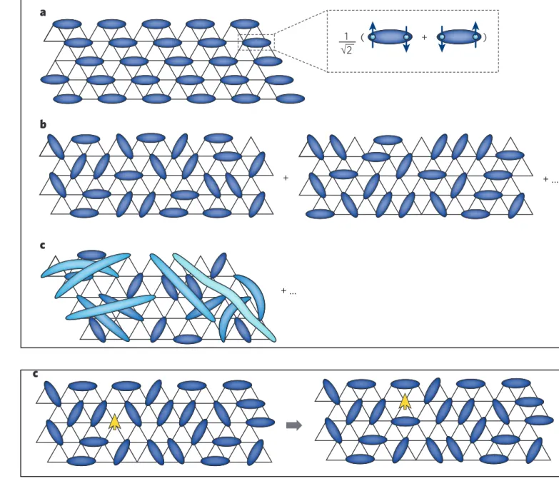
A natural building block for non-magnetic states is the valence bond, a pair of spins that, owing to an antiferromagnetic interaction, forms a spin-0 singlet state (Fig. 3a). A valence bond is a highly quantum object, the two spins being maximally entangled and non-classical. If all of the spins in a system are part of valence bonds, then the full ground state has spin 0 and is non-magnetic. One way in which this can occur is by the partitioning of all of the spins into specific valence bonds, which are static and localized. Mathematically, such a ground state is well approximated as a product of the valence bonds, so that each spin is highly entangled with only one other, its valence-bond partner. This is known as a valence-bond solid (VBS) state (Fig. 3a) and occurs in several materials^23–25. VBS states are interesting because, for instance, they provide an experimental way of studying Bose–Einstein condensation of magnons (which are triplet excitations of the singlet valence bonds) in the solid state²⁶.

A VBS state is not, however, a true QSL, because it typically breaks lattice symmetries (because the arrangement of valence bonds is not unique) and lacks long-range entanglement. To build a QSL, the valence bonds must be allowed to undergo quantum mechanical fluctuations.

The ground state is then a superposition of different partitionings of spins into valence bonds (Fig. 3b, c). If the distribution of these partition- ings is broad, then there is no preference for any specific valence bond and the state can be regarded as a valence-bond ‘liquid’ rather than a solid. This type of wavefunction is generally called a resonating valence- bond (RVB) state²². RVB states became subjects of intense theoretical interest when, in 1987, Anderson proposed that they might underlie the physics of high-temperature superconductivity⁴. Only relatively recently, however, have RVB wavefunctions been shown to be ground states of many specific model Hamiltonians^27–32.

It is now understood that not all QSLs are alike. Generally, different states have different weights of each valence-bond partition in their wavefunctions. The valence bonds need not be formed only from nearby

spins³³. If a valence bond is formed from spins that are far apart, then those spins are only weakly bound into a singlet and the valence bond can be ‘broken’ to form free spins with relatively little energy. So states that have a significant weight from long-range valence bonds have more low- energy spin excitations than states in which the valence bonds are mainly short range (see, for example, ref. 34). There are also other excitations that do not break the valence bonds but simply re arrange them. Such excita- tions can have low energy even in short-range RVB states.

Given the possibility of different QSL states, it is interesting to attempt to classify these states. This problem is only partly solved, but it is clear that the number of possible states is huge, if not infinite. For instance, Wen has classified hundreds of different ‘symmetrical spin liquids’

(QSLs with the full space-group symmetry) for S = ½ antiferromagnets on the square lattice³⁵. Finding the correct QSL ground state among all of the many pos sible RVB phases, many of which have similar energies, is a challenge to theory, reminiscent of the landscape problem in string theory, in high-energy physics.

Even with this diversity of possible states, one feature that theorists expect QSLs to have in common is that they support exotic excitations.

What is meant by exotic? In most phases of matter, all of the excitations can be constructed from elementary excitations that are either electron- like (spin S = ½ and charge ±e) or magnon-like (spin S = 1 and charge neutral). Only in rare examples, such as the fractional quantum Hall states, do the elementary excitations differ from these, in this case by carrying fractional quantum numbers. The magnetic monopoles in spin

A triangle of antiferromagnetically interacting Ising spins, which must point upward or downward, is the simplest example of frustration. All three spins cannot be antiparallel. As a re sult, instead of the two ground states mandated by the Ising symmetry (up and down), there are six ground states (see figure; blue circles denote magnetic ions, arrows indicate the direction of spin, and black and red lines indicate the shape of the triangular lattice, with red lines denoting the axis on which the spins are parallel). On 2D and 3D lattices, such degeneracies can persist.

When they do, fluctuations are enhanced and ordering is suppressed.

On the basis of this fact, Ramirez introduced a simple empirical measure of frustration that has become widely used⁵⁰. At high temperatures, the spin (or magnetic) susceptibility of a local-moment magnet generally has a Curie–Weiss form, χ!≈ C/(T− ΘCW), where T is temperature and C is the Curie constant. This allows extraction of the Curie–Weiss temper ature, ΘCW,from a plot of 1/χ versus T. |ΘCW| provides a natural estimate for the strength of magnetic interactions (ΘCW!<!0 for an antiferromagnet) and sets the scale for magnetic ordering in an

unfrustrated material. By comparing the Curie–Weiss temper ature with the temperature at which order freezes, T_c, the frustration parameter, f, is obtained: f = |ΘCW|/T_c. Typically, f!>!5–10 indicates a strong suppression of ordering, as a result of frustration. For such values of f, the temperature range T_c!<!T!<!|ΘCW| defines the spin-liquid regime.

Box 1 | Elements of frustration

201

NATURE|Vol 464|11 March 2010 REVIEW INSIGHT

199-208 Insight - Balents NS.indd 201

199-208 Insight - Balents NS.indd 201 3/3/10 11:35:123/3/10 11:35:12

© 20 Macmillan Publishers Limited. All rights reserved10

Low temperature regime

Superposi4on of the ground state

Thermal fluctuations:

→ 𝑘

𝑇 ∝ magnitude of spin (half-integers of ℏ )

Suppression of magne4c ordering

Spin liquid:

• Absence of long-range magne0c order

• No spontaneous symmetry breaking

• Liquid of disordered spins

“Spins can be thought of as a reordering randomly with 4me, cycling through different microstates. “

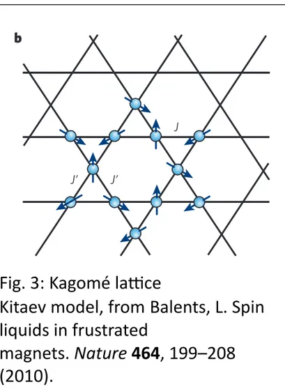
Fig. 3: Kagomé laUce

Kitaev model, from Balents, L. Spin liquids in frustrated

magnets. Nature 464, 199–208 (2010).

a

b

c

J’ J’

J

J’ J’

J

these configurations and the positions of protons in the tetrahedrally coordinated O²⁻ framework of water ice¹⁰.

When kBT << Jeff, the system fluctuates almost entirely within the two-in and two-out manifold of states. It turns out that the number of such states is exponentially large, so a low-temperature entropy remains even within this limit. This entropy, first estimated by Pauling in 1935 (ref. 11), has been measured in spin ice¹⁰. Although the spins remain paramagnetic in this regime, the ‘ice rules’ imply strong correlations:

for instance, if it is known that two spins on a tetrahedron are pointing out, then the other two spins must point in. The correlated paramagnet is a simple example of a classical spin liquid. A key question is whether the local constraints have long-range consequences: is the spin liquid qualitatively distinguishable from an ordinary paramagnet? Interest- ingly, the answer for spin ice is ‘yes’.

Analogies to electromagnetism

To understand how long-range effects arise from a local constraint, it is helpful to use an analogy to electromagnetism. Each spin can be thought of as an arrow pointing between the centres of two tetrahedra (Fig. 2b). This defines a vector field of flux lines on the lattice, which

because of the two-in, two-out rule is divergence free. In this sense, the vectors de fine an ‘artificial’ magnetic field, b, on the lattice (the field can be taken to have unit magnitude on each link, with the sign determined by the arrows). Because the spins are not ordered but fluctuating, the magnetic field also fluctuates. However, because the magnetic field lines do not start or end, these fluctuations include long loops of flux (Fig. 2b) that communicate spin correlations over long distances.

The nature of the long-distance spin correlations was derived by Young- blood and colleagues in a mathematically analogous model of a fluctuating ferroelectric, in which the electric polarization is similarly divergence- less¹²; this was subsequently rederived for spin ice¹³. The result is that the artificial magnetic field, at long wavelengths, fluctuates in equilibrium just as a real magnetic field would in a vacuum, albeit with an effective mag- netic permeability. For the spins in spin ice, this implies power-law ‘dipo- lar’ correlations that are anisotropic in spin space and decay as a power law (~1/r³, where r is the distance between the spins) in real space. It is remarkable to have power-law correlations without any broken symmetry and away from a critical point. After Fourier transformation of these cor- relations on the lattice, a static spin structure factor with ‘pinch points’ at reciprocal lattice vectors in momentum space is obtained^12–14.

Such dipolar correlations have recently been observed in high resolu tion neutron-scattering experiments by Fennell and colleagues¹⁵. At the pinch points, if the ice rules are obeyed perfectly, a sharp singular- ity is expected, as well as a precise vanishing of the scattering intensity along lines passing through the reciprocal lattice vectors. The rounding of this singu larity gives a measure of the ‘spin-ice correlation length’, which is estimated to grow to 2–300 Å (a large number) at a temperature of 1.3 K. In the future, it may be interesting to see how this structure changes at even lower temper atures, at which spin ices are known to freeze and fall out of equilibrium. Although the argument of Young- blood and colleagues¹² and the model outlined above rely on equilib- rium, arguments by Henley suggest that the pinch points could persist even in a randomly frozen glassy state¹⁴.

Magnetic monopoles

Interestingly, the magnetostatic analogy goes beyond the equilibrium spin correlations. One of the most exciting recent developments in this area has been the discovery of magnetic monopoles in spin ice¹⁶. These arise for simple mi croscopic reasons. Even when kBT << Jeff, violations of the two-in, two-out rule occur, although they are costly in energy and, hence, rare. The sim plest such defect consists of a single tetrahedron with three spins pointing in and one pointing out, or vice versa (Fig. 2c).

This requires an energy of 2Jeff relative to the ground states. From a magnetic viewpoint, the centre of this tetrahedron becomes a source or sink for flux, that is, a magnetic monopole. A monopole is a somewhat non-local object: to create a monopole, a semi-infinite ‘string’ of spins must be flipped, starting from the tetrahedron in question (Fig. 2c).

Nevertheless, when it has been created, the monopole can move by single spin flips without energy cost, at least when only the dominant nearest-neighbour exchange, Jeff, is considered.

Remarkably, the name monopole is physically apt: this defect carries a real ‘magnetic charge’¹⁶. This is readily seen because the physical mag- netic moment of the rare-earth atom is proportional to the pseudo- magnetic field, M = gμBb, where g is the Landé g factor and μB is the Bohr magneton. Thus, a monopole with the non-zero divergence =•b also has a non-zero =•M. The ac tual magnetic charge (which measures the strength of the Coulomb inter action between two monopoles) is, how- ever, small: at the same distance, the magnetostatic force between two monopoles is approximately 14,000 times weaker than the electrostatic force between two electrons. Nevertheless, at low temperatures, this is still a measurable effect.

A flood of recent papers have identified clear signatures of magnetic monopoles in new experiments and in previously published data. Jaubert and Holdsworth showed that the energy of a monopole can be extracted from the Arrhe nius behaviour of the magnetic relaxation rate¹⁷. They found that in Dy2Ti2O7 the energy of a monopole is half that of a single spin flip, reflecting the fractional character of the magnetic monopoles.

Figure 1 | Frustrated magnetism on 2D and 3D lattices. Two types of 2D lattice are depicted: a triangular lattice (a) and a kagomé lattice (b). The 3D lattice depicted is a pyrochlore lattice (c). In experimental ma terials, the three-fold rotational symmetry of the triangular and kagomé lattices may not be perfect, allowing different exchange interactions, J and Jʹ, on the horizontal and diagonal bonds, as shown. Blue circles denote magnetic ions, arrows indicate the direction of spin and black lines indicate the shape of the lattice. In b, ions and spins are depicted on only part of the illustrated lattice.

200

NATURE|Vol 464|11 March 2010

INSIGHT REVIEW

199-208 Insight - Balents NS.indd 200

199-208 Insight - Balents NS.indd 200 3/3/10 11:35:083/3/10 11:35:08

© 20 Macmillan Publishers Limited. All rights reserved10

Quantum spin liquid (QSL):

• small spin 𝑆 ≈ ^ℏ_$

• Long-range entanglement btw. the spins

• Exo@c excita@ons (frac@onal spin excita@ons: e.g. spinons)

Classical spin liquid:

• large spin 𝑆 ≫ ^ℏ_$

At small temperature the spins freeze or order.

Quantum spin liquids preserves its disorder to 𝑇 = 0 𝐾 due to the

uncertainty principle

How is a QSL iden<fied in experiments?

Candidate Materials

field. This model, as in Eq. 1, is named the Kitaev model.

H ¼ "K_x X

xbonds

S^x_i S^x_j " K_y X

ybonds

S^y_i S^y_j " K_z X

zbonds

S^z_iS^z_j: (1)

Here, H is the Hamiltonian and K_x,y,z are the nearest-neighbour Ising- type spin interactions along the x, y and zbonds (Kitaev interactions).

It has been shown that the exact ground state of the Kitaev model is a QSL, which may be gapped or gapless depending on the relative strength of the Kitaev interactions along the three bonds.¹³ Unlike QSLs described by the RVB model, the QSL state in the Kitaev model (Kitaev QSL hereafter) is defined on the honeycomb lattice where geometrical frustration is absent. Instead, the presence of bond- dependent Kitaev interactions induces strong quantum fluctuations that frustrate spin configurations on a single site, resulting in a Kitaev QSL state.

The Kitaev model is simple and beautiful but was considered as a ‘toy’ model in the beginning, since the underlying anisotropic Kitaev interactions are unrealistic for a spin-only system. One brilliant proposal to realize the Kitaev interaction is to include the orbital degree of freedom in a Mott insulator that arises from the combination of the crystal electric field, spin–orbital coupling (SOC), and electron correlation effects.¹⁴ A Mott insulator is an insulator that band theory predicts to be metallic, but turns out to be insulating due to electron–electron interactions.¹⁵ In the proposal,¹⁴ the electronic configuration is a consequence of the following processes: First, the octahedral crystal field splits the d orbitals into triply degenerate t_2g and doubly degenerate e_g orbitals at low and high energies, respectively; second, in the presence of strong SOC, the degeneracy of the t_2g is lifted, giving rise to one effective spin J_eff= 1/2 and one J_eff=3/2 band, both of which are entanglements of the S=1/2 spin and L_eff= −1 orbital moment for t_2g; third, the resulting J_eff=1/2 band is narrower than the original triply degenerate t_2g band. Consequently, a moderate electron correlation will open a gap and split this band into a lower and upper Hubbard band. Such a state is a J_eff= 1/2 Mott insulator. Due to the spatial anisotropy of the d orbitals and strong SOC, the exchange couplings between the effective spins are intrinsically anisotropic and bond dependent, and will give rise to the Kitaev interactions under certain circumstance.^13,14 These advancements bring the hope to find Kitaev QSLs in real materials, and have motivated intensive research in searching for QSLs beyond the triangular, kagome and pyrochlore lattices in recent years.^16,17

WHY QSLS ARE OF INTEREST

QSL is a highly nontrivial state of matter. Ordinary states are often understood within Landau’s framework in terms of order, phase transition and symmetry breaking. However, a QSL does not have a local order parameter and avoids any spontaneous symmetry breaking even in the zero-temperature limit, so to understand it requires theories beyond Landau’s phase transition theory. In fact,

?

?

J a

K K K

d c

b

Fig. 1 Schematics of some typical two-dimensional crystal structures on which quantum spin liquids may be realized. a, b Triangular, c Kagome, and d Honeycomb structures. Arrows and question marks represent spins and undetermined spin configurations due to geometrical frustration, respectively.J is the Heisenberg exchange interaction, and K_x,y,z are Kitaev interactions along three bonds. The shades illustrate spin singlets with a total spin S=0, each formed by two spins antiparrallel to each other

Table 1. Geometrically frustrated quantum-spin-liquid candidates

Material Structure Θcw (K) J (K) Reference

κ-(BEDT-

TTF)₂Cu₂(CN)₃ Triangular −375 250 ⁸⁴

EtMe₃

Sb[Pd(dmit)₂]₂ Triangular −(375−330) 220–250 ⁸⁵

YbMgGaO₄ Triangular −4 1.5 ³²

1T-TaS₂ Triangular −2.1 0.1 ⁸⁶

ZnCu₃(OH)₆Cl₂

(herbertsmithite) Kagome −314 170 ⁸⁷

Cu₃Zn(OH)₆FBr

(barlowite) Kagome −200 170 ⁸⁸

Na₄Ir₃O₈ Hyperkagome −650 430 ²⁷

PbCuTe₂O₆ Hyperkagome −22 15 ²⁸

Ca₁₀Cr₇O₂₈ Distorted kagome −9 ³⁴

Θcw and J are the Curie–Weiss temperature and exchange coupling constant, respectively

*Notes:

κ-(BEDT-TTF)₂Cu₂(CN)₃: With a J~ 250 K, no magnetic order nor spin freezing is observed down to 20 mK,⁸⁹ giving rise to a frustration index over 10,000. While low-temperature specific heat measurements indicate the presence of gapless magnetic excitations,⁶² they do not contribute to the thermal conductivity⁶³

YbMgGaO₄: A frequency-dependent peak in the a.c. susceptibility characteristic of a spin glass is observed around 0.1 K³³

1T-TaS2: Note thatΘcwandJlisted in the table are significantly smaller than those calculated from the high-temperature susceptibility in ref. ³⁵ In 1T- TaS₂, 13 Ta⁴⁺ ions form a hexagonal David star cluster when the system is cooled below the commensurate charge density wave phase transition temperature at 180 K.⁹⁰ Twelve Ta⁴⁺ ions in the corner of the star form six covalent bonds and the spins connected by the bonds cancel out. An orphan electron is localized in the centre of the David star, giving rise to a net spin of S=1/2 for each David star. The spins in the centre constitute a triangular network, making the system essentially a geometrically frustrated magnet. At present, whether or not this material is a QSL is still under hot debate^{35,86,90–92}

Na4Ir3O8: Although a well-defined magnetic phase transition is not observed in Na4Ir3O8, a spin-glass transition occurs around 6 K, below which the spins are frozen and maintain short-range correlations^27,93,94 Ca₁₀Cr₇O₂₈: It is a system with complex structure, and more interestingly, with dominant ferromagnetic interactions.³⁴ Frequency-dependent peak was observed in the a.c. susceptibility, suggestive of a spin-glass ground state, but it is suggested that such a state could be ruled out by performing the Cole–Cole analysis on the a.c. susceptibility data.³⁴

J. Wen et al.

2

npj Quantum Materials (2019) 12 Published in partnership with Nanjing University

1234567890():,;

most QSLs are believed to be associated with topological order and phase transition.^18,19

QSLs are Mott insulators where the bands are half filled, and different from band insulators, where the bands are fully filled or empty. Here, the electron–electron correlation is important, and the conventional band theory with the single-particle approxima- tion does not work well.^20,21 Therefore, understanding QSLs should and has already provided deep insights into the rich physics of strongly correlated electron systems. Moreover, in 1987, a year after high-temperature superconductivity was discovered in copper oxides,²² P.W. Anderson²³ proposed that the parent compound, a Mott insulator La₂CuO₄, which by doping with carriers can superconductivity be achieved, was a QSL. This proposal injects significant momentum into the research of QSLs as it may lend support to solve the puzzle of high-temperature superconductivity.¹⁵

Besides the fascinating physics associated with QSLs, they also hold great application potentials. For example, in a QSL, the spins are entangled over a long range, which is an essential ingredient for quantum communication.²⁴ Another important property of a QSL associated with the long-range entanglement is the presence of fractional spin excitations. For instance, a Kitaev QSL can support fractional excitations represented by Majorana fermions, which can be made to behave as anyons obeying the non-Abelien statistics in the presence of magnetic field.¹³ Braiding these anyons is an important step towards the topological quantum computation.²⁵

CANDIDATE MATERIALS

Motivated by the rich physics and fascinating properties of QSLs, studying these materials has been a 45-year long but still dynamic field. There has been a lot of progress made both on the theoretical and experimental aspects. QSLs in one-dimensional magnetic chain have been well established and will not be discussed in this work. For reference, there is a recent review article in this topic in ref. ²⁶ Here, we will focus on QSLs in two or three dimensions. There have been many theoretical proposals for QSLs. For details, please refer to the reviews and references therein.^5,6,17

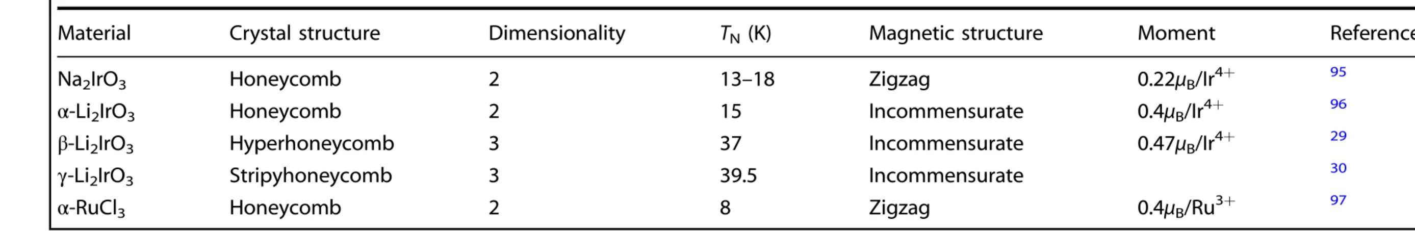
Experimentally, numerous materials have been suggested to be candidates for QSLs, some of which are tabulated in Table 1 and Table 2. We classify these materials into two categories— geometrically frustrated materials where the RVB model is applicable (Table 1) and Kitaev QSL candidates where the Kitaev physics is relevant (Table 2). For the majority of these materials, the discussions of QSL physics are in two dimensions, where the reduced dimensionality enhances quantum fluctuations needed for QSLs. In recent years, there have also been attempts to look for three-dimensional QSL candidates, such as hyperkagome Na4Ir3O8

(ref. ²⁷) and PbCuTe₂O₆,²⁸ hyperhoneycomb β-Li₂IrO₃,²⁹ and stripyhoneycomb γ-Li₂IrO₃.³⁰ A more detailed review on the search of three-dimensional QSLs can be found in ref. ¹⁷

HOW TO IDENTIFY A QSL EXPERIMENTALLY Technique overview

Strictly speaking, to identify a QSL, one should perform measure- ments at absolute zero temperature, which is not practical. As a common practice, it is often assumed that when the measuring temperature T is far below the temperature, which characterizes the strength of the magnetic exchange coupling, say two orders of magnitude for instance, thefinite-temperature properties can be a representation of those of the zero-temperature state, provided that there is no phase transition below the measuring tempera- ture. Even so, experimental identification of a QSL is still challenging since a QSL does not spontaneously break any lattice symmetry and no local order parameter exists to describe such a state. One first step is to prove that there is no magnetic order nor spin freezing down to the lowest achievable temperature in, preferably, low-spin systems whose spin interactions are dom- inantly antiferromagnetic. For example, measuring the magnetic susceptibility is very useful in this aspect. By performing a Curie–Weiss fit to the high-temperature magnetic susceptibility, one can also obtain the Curie–Weiss temperature Θ_CW that characterizes the strength of the antiferromagnetic interactions.

We list the Θ_CW and exchange coupling constant J for some materials in Table 1.

Specific heat is also quite often measured to help screen a QSL.

For a material that orders magnetically at low temperatures, a λ- type peak in the specific heat vs. temperature curve is generally expected. By contrast, for a QSL, such a sharp peak is typically absent, unless in the case such as that there is a topological phase transition.³¹ Furthermore, it also reveals that whether there exist finite magnetic excitations at low temperatures or not. The residual magnetic entropy can be calculated, provided that the phonon contribution to the specific heat can be properly subtracted, ideally by subtracting the specific heat of a proper nonmagnetic reference sample. By examining how much entropy has already been released at the measuring temperature, the possibility of establishing a long-range magnetic order at a lower temperature can be estimated.^32,33 In addition to these macro- scopic measurements, microscopic probes such as muon spin relaxation (µSR) and nuclear magnetic resonance (NMR) that are sensitive to the local magnetic environment are also often used to detect whether there is spin ordering or freezing.^34–36 Neutron diffraction can also tell explicitly whether a system is magnetically ordered or not.

These measurements reveal very important information, but are not completely satisfactory, partly because: even though magnetic ordering can be excluded, such a ground state without a long- range order may be caused by the disorder, which leads to a percolative breakdown of the long-range order. In such a case, the spin-liquid-like state is similar to a classical spin liquid, but essentially different from a QSL. So, are there better approaches that can identify a QSL more directly from a positive aspect?

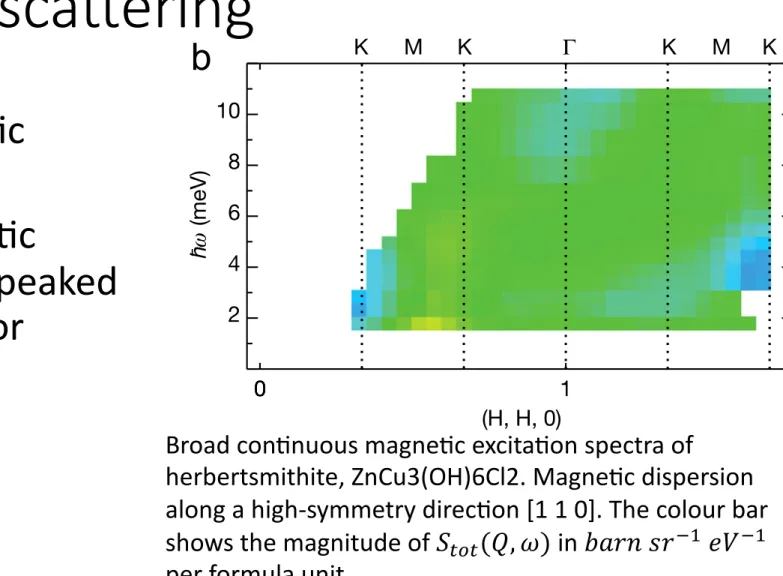
The key features defining a QSL are the long-range entangle- ment and the associated fractional spin excitations. At present, it is hard to define and characterize the former, so the answer to this question mostly lies on the fractional excitations, for example, spinons predicted in the RVB model.³ Spinons are charge-neutral Table 2. Kitaev quantum-spin-liquid candidates

Material Crystal structure Dimensionality TN (K) Magnetic structure Moment Reference

Na2IrO3 Honeycomb 2 13–18 Zigzag 0.22μB/Ir^{4+ 95}

α-Li₂IrO₃ Honeycomb 2 15 Incommensurate 0.4μ_B/Ir^{4+ 96}

β-Li2IrO3 Hyperhoneycomb 3 37 Incommensurate 0.47μB/Ir^{4+ 29}

γ-Li₂IrO₃ Stripyhoneycomb 3 39.5 Incommensurate ³⁰

α-RuCl3 Honeycomb 2 8 Zigzag 0.4μB/Ru^{3+ 97}

J. Wen et al.

3

Published in partnership with Nanjing University npj Quantum Materials (2019) 12

From Wen, J., Yu, S., Li, S. et al. Experimental

idenAficaAon of quantum spin liquids. npj Quantum Mater. 4, 12 (2019).

Problem 1: Classifica<on of QSL – no local order parameter:

• Landau’s theory:

• A phase transi@on is simply a transi@on that changes the symmetry

• Characteriza@on: local order parameters (e.g. magne@za@on 𝑚), symmetry breaking etc.

• QSL phase is beyond the conven4onal phase transi4on

• Topological order:

• Characterized by a new set of tools: degeneracy of the ground state, QP sta@s@cs or edge states