Quantum Spin Liquids

Quantum Spin Liquids

on

in

Three-Dimensional Frustrated Magnets

Finn Lasse Buessen

Quantum Spin Liquids

in Three-Dimensional Frustrated Magnets

Inaugural-Dissertation zur

Erlangung des Doktorgrades

der Mathematisch-Naturwissenschaftlichen Fakult¨at der Universit¨at zu K¨oln

vorgelegt von

Finn Lasse B¨ ußen

aus Flensburg

K¨oln 2019

Priv.-Doz. Dr. Michael Scherer Prof. Dr. Ronny Thomale

Tag der m¨ undlichen Pr¨ ufung: 23.08.2019

When sizable quantum fluctuations and strong frustration mechanisms act in concert to repel the formation of conventional long-range order in quantum magnets, they can make way for massively entangled spin liquid phases which may imbue the material with extraordinary properties. The search for such curious phases of matter has proceeded for several decades, gaining extra momentum some fifteen years ago when Kitaev proposed an analytically solvable model for a quantum spin liquid with anyonic excitations on the basis of realistic microscopic spin exchange terms [Kitaev, Annals of Physics 321, 2 (2006)]. Attempts to identify different models or materials which harbor quantum spin liquid ground states have kept researchers – experimentalists and theorists alike – in suspense ever since. However, the simulation of quantum many-body systems poses a serious challenge even to modern numerical techniques, particularly in the case of frus- trated quantum magnetism in three spatial dimensions. Such models evade tractability by many established approaches, leaving a methodological void.

In this thesis, we report on recent progress in cutting-edge implementations of the pseudo-fermion functional renormalization group (pf-FRG), which has originally been proposed by Reuther and W¨olfle in the context of two-dimensional frustrated quantum magnetism with highly symmetric spin interactions [Reuther and W¨olfle, Phys. Rev. B 81, 144410 (2010)]. Reflecting the growing interest in models with SU(2) symmetry-breaking spin exchange terms that has followed the unearthing of Kitaev’s honeycomb model, we present a generalized implementation of the pf-FRG which is suited to numerically sim- ulate arbitrary microscopic models with diagonal or off-diagonal two-spin interactions, even in three-dimensional frustrated quantum magnets. We provide insight into the in- ner workings of the method which has emerged over the course of the last couple of years, arguing that the pf-FRG formalism simultaneously combines aspects of a large-S expan- sion as well as a large-N expansion on equal footing, thus being able to resolve the subtle interplay between magnetic ordering tendencies and disruptive quantum fluctuations.

Moreover, on a case by case basis we explore the stability of quantum spin liquids in paradigmatic models of frustrated quantum magnetism and elucidate the joint ac- tion of geometric frustration, exchange frustration, and quantum fluctuations to inhibit the formation of magnetic long-range order. Examples include: (i) a Heisenberg spin model on the three-dimensional diamond lattice where geometric frustration arises from antiferromagnetic next-nearest neighbor interactions. The additional competition with nearest neighbor interactions leads to an unusually large ground state degeneracy al- ready on classical level. The quantum-to-classical transition is studied by systematically varying the spin length and the different roles of quantum fluctuations and thermal fluctuations are discussed. The theory is applied to interpret experiments on the spin- liquid candidate NiRh2O4; (ii) a Heisenberg antiferromagnet on the face centered cubic

uation is identified where both mechanisms collude to give rise to an unusually large degree of frustration over a wide parameter regime. We discuss related experimental findings on the highly frustrated iridate compound Ba2CeIrO6; (iii) a Heisenberg anti- ferromagnet on the kagome lattice with additional Dzyaloshinskii-Moriya interactions.

The robustness of the unperturbed kagome antiferromagnet’s spin liquid ground state against low-symmetry Dzyaloshinskii-Moriya interactions is investigated. Implications for the spin-liquid candidate herbertsmithite are discussed.

Wenn starke Quantenfluktuationen und Frustrationsmechanismen mit geeinten Kr¨aften die Bildung von konventioneller langreichweitiger Ordnung verhindern, k¨onnen statt- dessen massiv verschr¨ankte Spinfl¨ussigkeitszust¨ande entstehen, die dem Material au- ßerordentliche Eigenschaften verleihen. Die Suche nach solch merkw¨urdigen Zust¨anden in Materie l¨auft seit einigen Jahrzenten; Besonderen Nachdruck verliehen hat ihr vor etwa 15 Jahren die Entdeckung eines analytisch exakt l¨osbaren Modells einer Quanten- spinfl¨ussigkeit mit anyonischen Anregungszust¨anden und realistischen mikroskopischen Kopplungen durch Kitaev [Kitaev, Annals of Physics 321, 2 (2006)]. Die Bem¨uhungen, verschiedene Modelle und Materialien zu identifizieren, die Spinfl¨ussigkeits-Grundzu- st¨ande beherbergen, hat Forscher – Theoretiker und Experimentalphysiker gleicherma- ßen – seitdem in Atem gehalten. Allerdings stellt die Simulation von Quantenvielteil- chensystemen sogar f¨ur moderne numerische Techniken eine große Herausforderung dar, insbesondere im Falle von frustriertem Quantenmagnetismus in drei r¨aumlichen Dimen- sionen. Derartige Modelle entziehen sich einer Beschreibung durch viele konventionelle Ans¨atze und sind daher methodisch schwer zug¨anglich.

In dieser Arbeit berichten wir ¨uber aktuelle Fortschritte in modernen Implementie- rungen der pseudo-fermionischen funktionellen Renormierungsgruppe (pf-FRG), welche urspr¨unglich von Reuther und W¨olfle im Kontext von zweidimensionalem Quantenma- gnetismus mit hochsymmetrischen Wechselwirkungen eingef¨uhrt wurde [Reuther und W¨olfle, Phys. Rev. B 81, 144410 (2010)]. Wir pr¨asentieren, das wachsende Interesse an SU(2)-symmetriebrechenden Spinwechselwirkungen widerspiegelnd welches auf die Entdeckung von Kitaevs Honigwabenmodell zur¨uckgeht, eine verallgemeinerte Formu- lierung der pf-FRG, die imstande ist, beliebige mikroskopische Modelle mit diagonalen oder nicht-diagonalen paarweisen Spinwechselwirkungen numerisch abzubilden – sogar Modelle von dreidimensionalem frustrierten Magnetismus. Wir setzen uns mit Erkennt- nissen zur Funktionsweise der Methode auseinander, die im Laufe der vergangenen Jahre gewonnen werden konnten, und argumentieren dass der pf-FRG-Formalismus auf gleich- berechtigte Art verschiedene Aspekte von systematischen Reihenentwicklungen in der Spinl¨ange und der Spinsymmetrie verbindet, was dessen F¨ahigkeit begr¨undet, das sub- tile Zusammenspiel von magnetischen Ordnungstendenzen und Unordnung schaffenden Quantenfluktuationen aufzul¨osen.

Außerdem untersuchen wir anhand von aussagekr¨aftigen Fallbeispielen die Stabi- lit¨at von Quantenspinfl¨ussigkeiten und er¨ortern das Zusammenwirken von geometrischer Frustration, Austauschfrustration und Quantenfluktuationen im Hinblick auf die Un- terdr¨uckung von langreichweitiger magnetischer Ordnung. Die Fallbeispiele umfassen:

(i) Ein Heisenberg-Modell auf dem dreidimensionalen Diamantgitter, welches mit geo- metrischer Frustration versehen ist, die auf antiferromagnetische ¨Ubern¨achste-Nachbar-

zustandsentartung. Der ¨Ubergang vom klassischen Fall zum Quantenfall wird unter- sucht indem systematisch die Spinl¨ange variiert wird, und es werden die unterschied- lichen Auswirkungen von Quantenfluktuationen und thermischen Fluktuationen disku- tiert. Das Modell wird herangezogen, um Experimente an dem Spinfl¨ussigkeitskandidaten NiRh2O4 zu interpretieren; (ii) Einen Heisenberg-Antiferromagneten auf dem kubisch fl¨achenzentrierten Gitter, welcher mit zus¨atzlichen richtungsabh¨angigen Wechselwirkun- gen versehen ist und somit gleichzeitig geometrische Frustration und Austauschfrustrati- on aufweist. Es wird eine Bedingung identifiziert, unter der sich beide Mechanismen ge- genseitig verst¨arken und zu ungew¨ohnlich starker Frustration ¨uber einen großen Parame- terbereich f¨uhren. Der Bezug zu Experimenten an dem hochfrustrierten Iridat Ba2CeIrO6

wird hergestellt; (iii) Einen Heisenberg-Antiferromagneten auf dem Kagome-Gitter mit zus¨atzlichen Dzyaloshinskii-Moriya-Wechselwirkungen. Die Stabilit¨at der urspr¨unglich- en Kagome-Spinfl¨ussigkeit gegen¨uber den niedrigsymmetrischen Dzyaloshinskii-Moriya- Wechselwirkungen wird untersucht. Die Implikationen f¨ur den Spinfl¨ussigkeitskandidaten Herbertsmithit werden thematisiert.

1. Introduction 9

1.1. Recurring motifs in spin liquids . . . 12

1.1.1. Classical spins . . . 12

1.1.2. Order by disorder . . . 13

1.1.3. Quantum spins . . . 13

1.1.4. Quantum fluctuations . . . 14

1.1.5. Resonating valence bonds . . . 16

1.1.6. Frustration . . . 19

1.2. Simulation techniques for spin liquids . . . 21

1.2.1. Exact diagonalization . . . 21

1.2.2. Quantum Monte Carlo . . . 22

1.2.3. Density matrix renormalization group . . . 23

1.2.4. Functional renormalization group . . . 25

2. The pseudo-fermion functional renormalization group 27 2.1. Functional renormalization group . . . 29

2.2. The pseudo-fermion Hamiltonian . . . 36

2.2.1. U(1) gauge redundancy . . . 38

2.2.2. Particle-hole gauge redundancy . . . 40

2.2.3. Lattice symmetries . . . 41

2.2.4. Time-reversal symmetry . . . 42

2.2.5. Hermitian symmetry . . . 44

2.2.6. Implications on vertex functions . . . 44

2.3. Pseudo-fermion functional renormalization group . . . 49

2.3.1. Flow equations . . . 50

2.3.2. Observables . . . 55

2.3.3. Pr´ecis . . . 56

2.4. Numerical solution of the flow equations . . . 58

2.4.1. Differential equation solver . . . 58

2.4.2. Matsubara frequency discretization . . . 60

2.4.3. Lattice size . . . 62

2.4.4. Computational complexity . . . 65

2.5. Methodological case studies . . . 67

2.5.1. Phase transitions . . . 67

2.5.2. Katanin truncation . . . 69

2.5.3. Flow equations with extra symmetries . . . 71

2.5.4. Quantum limit at large N . . . 74

2.5.5. Classical limit at large S . . . 77

2.5.6. Finite temperature . . . 80

2.5.7. Pr´ecis and future prospects . . . 83

3. Frustrated magnets and quantum spin liquids 85 3.1. Quantum spiral spin liquids . . . 85

3.1.1. Minimal model and classical spins . . . 87

3.1.2. Quantum order by disorder . . . 90

3.1.3. Thermodynamics of quantum spiral spin liquids . . . 92

3.1.4. Application to NiRh2O4 . . . 100

3.1.5. Summary . . . 104

3.2. Magnetic order from Kitaev interactions . . . 105

3.2.1. Minimal model . . . 105

3.2.2. Frustration parameter . . . 109

3.2.3. Application to Ba2CeIrO6 . . . 111

3.2.4. Summary . . . 113

3.3. Dzyaloshinskii-Moriya interactions in herbertsmithite . . . 114

3.3.1. Out-of-plane DM interactions . . . 115

3.3.2. In-plane DM interactions . . . 117

3.3.3. Application to herbertsmithite . . . 117

3.4. Pr´ecis . . . 119

4. Concluding remarks 121 A. Pf-FRG flow equations 125 A.1. SU(N) Heisenberg model . . . 125

A.2. Spin-S Heisenberg model . . . 128

A.3. Off-diagonal spin interactions . . . 129

Bibliography 139

Quantum spin liquids are curious phases of matter in which the proliferation of mag- netic order is impeded by the presence of strong quantum fluctuations even at lowest temperatures down to absolute zero. The term quantum spin liquid is a tribute to the early observation that magnetic moments in such a phase of matter, despite exhibiting strong short-range correlations, seem to remain disordered across longer distances – just like particles in a conventional liquid. Yet, while the absence of magnetic long-range order is a pivotal aspect of quantum spin liquids, it constitutes only a negative defini- tion, characterizing what a spin liquid is not – and, more importantly, it conceals the significant progress that has been achieved in carving out the extraordinary properties of quantum spin liquids that by no means can be associated with conventional liquids.

Converging towards a universal, positive definition of quantum spin liquids remains dif- ficult, but some aspects have received a great deal of attention in the past: (i) quantum spin liquids are understood to be highly entangled states of matter, (ii) they have the ability to host non-local excitations which are associated with the fractionalization of the original spin degrees of freedom and emergent gauge fields, and (iii) they can have topological properties [1, 2].

All three aspects are intimately linked to each other by the implication of non-locality.

The property of massive entanglement can be understood to guarantee that any finite part of the system cannot be smoothly connected to a simple product state, which is essential in order to enable the system to host non-local excitations, quasiparticles, whose appearance can be explained in a framework of fractionalization of the original degrees of freedom into a new type of particle, partons, that live in the background of an emergent gauge field. The partons may carry fractional quantum numbers and have decisively different physical properties than any of the constituents in the original physical system.

In particular, their physical properties can be of a form which cannot be generated from any finite number of local operators in the original model – if the latter was the case, the parton state could be labeled by a combination of all quantum numbers involved in the sequence of local operations, and the composite operator would consequently describe a well-defined object that has a finite spatial extent. This would be at odds with the emergent partons’ ability to have non-trivial exchange statistics, requiring them to ‘sense’ each others presence at arbitrary distance [1]. Similar reasoning holds for the relation between entanglement and the formation of topological properties – which are, by definition, non-local [3].

Being at the foundation of many fascinating, yet intricate, many-body phenomena, the inherently quantum mechanical nature of highly entangled states of matter also implies great challenges in their analysis in terms of analytic approaches as well as numerical simulations. Despite these deep-rooted difficulties, unparalleled insight into

the phenomenology of quantum spin liquids has been drawn from the revelation of the much celebrated Kitaev honeycomb model [4]. Being amenable to an exact solution, direct investigation of the fractionalization process of the original spin degrees of freedom into emergent Majorana fermions and an accompanying staticZ2 gauge field is possible.

It was quickly appreciated that non-diagonal spin interactions of Kitaev type can be realized in actual materials, which has sparked formidable activity in the search for geniune Kitaev materials [5].

Yet the search for quantum spin liquids is neither constrained to the Kitaev honey- comb model nor to two-dimensional models. Various spin liquid candidates have also been identified in three-dimensional materials, where frustrated interactions and quan- tum fluctuations may remain sufficiently strong to defy magnetic order, despite the generally larger coordination numbers in higher dimensional lattice graphs. The the- oretical analysis of three-dimensional frustrated quantum magnets, however, poses a serious challenge to modern quantum many-body simulation techniques.

In this thesis, we attack the elusive field of three-dimensional frustrated quantum magnetism by adopting a functional renormalization group (pf-FRG) formalism which brings together aspects of modern quantum field theory and state of the art numerical techniques. The technique was first employed by Reuther and W¨olfle in 2010 [6] and has since been refined significantly. Many important results in this thesis go back to significant progress in method development around the pf-FRG approach. Consequently, the thorough review of the current state of the pf-FRG formalism as a tool for the simulation of frustrated quantum magnets is a central goal of this thesis.

However, equally important, this thesis is devoted to the exploration of frustrated quantum magnets and microscopic models thereof as potential platforms to stabilize spin liquid ground states, with a focus on three-dimensional models. Mediating at the interface between aesthetically pleasing minimal models which strive for maximum ele- gance and simplicity on the one hand, and intricate models which reflect the experimental reality of imperfect materials and the involvement of unfavorable spin exchange terms on the other hand, we are interested in the stability of quantum spin liquid phases under perturbations of the underlying models. Any knowledge about the stability of spin liq- uid regimes and the relevance of perturbations provides valuable guidance for material design and contributes to our chances to unveil new materials which can cultivate spin liquid ground states.

We specifically address three different incarnations of frustrated quantum magnets, where in each case we formulate a microscopic model, make predictions based on pf- FRG simulations, and relate the predictions to experiment: (i) We address a model of Heisenberg spins on the diamond lattice, where geometric frustration arises from anti- ferromagnetic next-nearest neighbors. We illustrate the formation of a quantum spiral spin liquid ground state that benefits from an unconventionally large classical ground- state degeneracy whose details depend on the precise ratio of involved nearest neighbor and next-nearest neighbor spin interactions. We resolve the connection between the quantum model and the classical limit in greater detail by systematically manipulating the spin length, in order to trace the subtle competition between disordering quantum

have been reported. (ii) We address a model of antiferromagnetic Heisenberg interactions on the face centered cubic lattice which are augmented by additional bond-directional Kitaev-like exchange couplings. We focus on the concurrent manifestation of geometric frustration and exchange frustration, and we identify a parameter regime where both mechanism collude to give rise to an unusually large degree of frustration. We invoke this theory on the spin-orbit entangled j = 1/2 iridate compound Ba2CeIrO6 to in- terpret recent experimental findings. (iii) Finally, we consider the kagome Heisenberg antiferromagnet in the presence of additional Dzyaloshinskii-Moriya interactions as an example of a model where off-diagonal spin interactions become relevant. The theory is applied to the kagome material herbertsmithite.

The remainder of this introductory chapter covers two complementary themes: what physical mechanisms may give rise to quantum spin liquids, and which techniques can be used to simulate microscopic models of frustrated quantum magnetism. The first question is addressed in Section 1.1, where we review a number of motifs which fre- quently appear in models and materials that ultimately harbor spin liquid phases. The aim of this section is to convey a feeling of what knobs and handles can be turned in an attempt to engineer spin liquid phases, or to push proximate spin liquid materials closer to a true quantum spin liquid ground state. We eventually follow up on these motifs in Chapter 3 where they make recurrent appearances in our studies of the various models of frustrated quantum magnetism mentioned above, and we shall indeed see how they give rise to quantum spin liquid ground states in realistic settings. The second question is addressed in Section 1.2, where we briefly review some of the most impor- tant methods and numerical approaches which researchers have been using in the past to study frustrated quantum magnets. The section is intended to provide context on the method development and to prepare for the review of the pseudo-fermion functional renormalization group, which is the main subject in Chapter 2 of the thesis.

1.1. Recurring motifs in spin liquids

While no sure formula exists to engineer quantum spin liquid phases, there are some guiding themes which have proven helpful in the search for this elusive phase of matter.

In this first section, we review several aspects that frequently seem to play a central role in finding ways to repel magnetic order. These facets include the role of classically degenerate ground states and thermal fluctuations, quantum fluctuations, resonating valence bonds, and frustration.

1.1.1 Classical spins. Classical spins are intuitive objects. A classical spin is conven- tionally associated with a vector in three-dimensional space, meaning that its configu- ration is uniquely determined by a length and a sense of orientation. By means of this identification one can adopt the formalism of vector calculus to model the interaction of two (or more) spins. A quantitative description of the interaction of spins is natu- rally given by their exchange energy – a number which determines whether a given local configuration is favorable (the configuration has a low exchange energy) or unfavorable (it has a high exchange energy). In many materials the exchange energy of two spins is modeled sufficiently well by assuming isotropic interactions, where the exchange energy is computed as the scalar product of two interacting spins. This model is referred to as the classical Heisenberg model and its Hamiltonian reads

H =X

i,j

Jij~si~sj , (1.1)

where~s_i and~s_j are vectors on the unit sphere representing (normalized) spins at lat- tice sites i and j, respectively. The interaction parameter Jij quantifies the interaction strength between pairs of spins. The sign of the coupling constant determines whether the exchange energy is minimized by a ferromagnetic state (Jij < 0) or an antiferro- magnetic configuration (Jij >0). The interaction constant can in principle be assigned an arbitrary value for any two pairs of spins, but for meaningful physical models it is constrained by symmetries of the underlying lattice. Furthermore, realistic interactions are often short-ranged since the magnitude of the effective interaction results from the overlap of localized electronic orbitals [7]. Yet, the exchange constants can also become long-ranged, e.g. in the presence of dipolar interactions [8], or in more exotic superstruc- ture materials [9]. In general, there is no upper limit for potential complications to add to the model. One can study anisotropies in the spin interaction, where the coupling constant is different for every component of the spins. One can study lattice anisotropies which strengthen or weaken interactions along certain lattice directions. One can study three-spin interactions, or even higher orders. One can add a magnetic field. There is a long list of more intricate models which have become popular enough to coin their own names. Any of these models can – and often do – give rise to a rich field of physics that is worth studying on its own. Some of the models aim at establishing unconventional forms of magnetic order [10], while other models aim at suppressing magnetic order altogether, giving way to potential spin liquid phases.

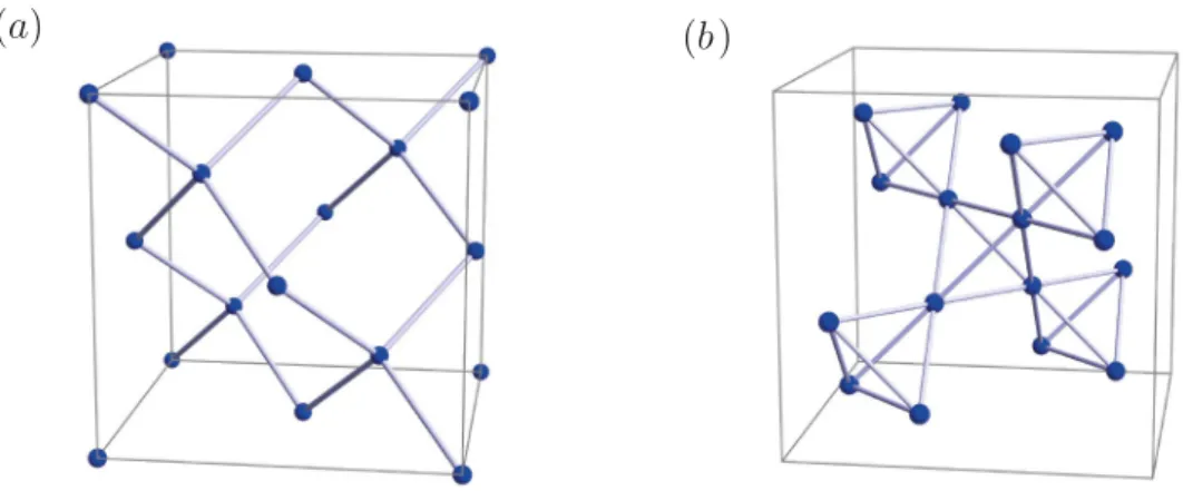
Figure 1.1. Order by disorder. (a) A degenerate manifold of states (black line) with ther- mally accessible excitations (blue region). Every configuration in the manifold is associated with the same number of thermally accessible excitations. (b) A subset of states in the degen- erate manifold has access to significantly more excited states (top left region of the manifold).

The larger entropy generated from the enhanced number of thermally accessible configurations reduces the free energy for certain configurations within the degenerate manifold, and those configurations are likely to be selected as the ground state of the system.

1.1.2 Order by disorder. Aiming for the cultivation of a spin liquid is challenging.

A classical spin liquid, which does not exhibit magnetic long-range order, arises from the presence of an extensively degenerate ground state which is often the result of fine tuning of parameters – as such it is fundamentally different from a quantum spin liquid, which can be captured by a single quantum mechanical wave function (we discuss this in the next sections). Sustaining an ensemble of degenerate states at non-zero temper- atures is even more challenging, since this does not just require the states to have the same energy, but it also requires the states to have similar excitations. If a subset of the degenerate states has lower excitations than the remaining configurations, those con- figurations will have a lower free energy since thermal fluctuations may occupy a more expansive number of excited states which results in a larger entropy (see Fig. 1.1). The subset of configurations which minimizes the free energy is likely to be selected as the ground state of the system. Therefore, thermal fluctuations can potentially stabilize a particular configuration of magnetic order out of an ensemble of otherwise degenerate states. Consequently, the mechanism was coined ‘order by disorder’ [11].

In Sec. 3.1, we discuss an exemplary model where order by disorder plays a decisive role. We make the connection between a classical version of the spin model, which hosts a (sub-)extensive number of degenerate ground state configurations, to the quantum ver- sion of the model, where thermal fluctuations are accompanied by quantum fluctuations.

We shall see that both, thermal fluctuations and quantum fluctuations lift the ground state degeneracy by means of order by disorder and quantum order by disorder, respec- tively. Yet, we shall further see that classical spins eventually undergo a thermal phase transition into magnetic long-range order while quantum order by disorder may not be strong enough to induce magnetic order, such that quantum spins remain fluctuating even at lowest temperatures.

1.1.3 Quantum spins. Within this thesis, we are interested in the study of spin liquids, more specifically quantum spin liquids. Promoting classical spins to quantum spins introduces quantum fluctuations which can help to suppress magnetic order, given that the ordering tendency is not too strong. In analogy to the classical Heisenberg model (1.1), the quantum version of the Heisenberg model is given by the Hamiltonian

H =X

i,j

JijS_iS_j . (1.2)

The quantum mechanical spin-1/2 moments are now represented by the operator-valued vectorsS_i with three componentsS_i^α, whereα ∈ {x, y, z}. Unlike in the classical model, the individual spin components no longer commute. Instead, they obey the commutation relations of the SU(2) algebra,

h

S_i^α, S_j^βi

=δijαβγS_i^γ , (1.3)

and can thus be represented in the basis of Pauli matrices S_i^α = 1

2σ^α , (1.4)

where the three Pauli matrices σ^α are given by σ^x =

0 1 1 0

σ^y =

0 −i i 0

σ^z =

1 0 0 −1

. (1.5)

This specific choice of representation in terms of hermitian 2×2 matrices implies that the spin operators act on the two-dimensional spinor space of spin-1/2 moments. The two dimensions of the spinor are identified with the two eigenstates of the S^z operator, which have eigenvalues +1/2 (spin up) and −1/2 (spin down). We denote these basis states as |↑i and |↓i, respectively, and refer to them as the S^z-basis. We shall remind ourselves at this point that the spin length is encoded in the dimensionality of the representation of the SU(2) group (which in this case is two), not in the choice of the symmetry group itself (which in this case is SU(2)). It is therefore possible to change the spin length and the spin symmetry independently; later on in this thesis, we explicitly construct SU(N) generalized spin models, see Sec. 2.5.4.

1.1.4 Quantum fluctuations. Two of the three components of a spin operator can equivalently be rewritten in terms of spin raising and lowering operators

S_i⁺ =S_i^x+iS_i^y S_i⁻ =S_i^x−iS_i^y , (1.6)

which are obtained as linear combinations of the original operators. They act on the basis states according to

S⁺|↑i= 0 S⁺|↓i=|↑i S⁻|↑i=|↓i S⁻|↓i= 0 . (1.7) As suggested by the naming, the spin raising operator can raise the z-component of a spin from −1/2 to +1/2, but it annihilates a +1/2 state. Conversely, the spin lowering operator changes a spin state +1/2 into−1/2. We may specify arbitrary spin configura- tions in the S^z-basis, such that they are eigenstates of theS^z operator by construction.

Yet, if the Hamiltonian of the microscopic spin model contains not only S^z operators it evidently generates transitions between different spin configurations via spin raising or lowering operations, and it is even likely to return superpositions of different configura- tions. These quantum fluctuations between different spin configurations can drive the system away from magnetic order and remain present down to zero temperature, where thermal fluctuations fade out.

The strength of quantum fluctuations depends on the spin length S, which we previ- ously assumed to be 1/2. In the limit of large spinsS → ∞the quantum fluctuations be- come irrelevant and one approaches the classical limit. We have pointed out in Sec. 1.1.3 that the spin length is represented by the dimensionality of the SU(2) representation;

generally, the dimensionality of the representation for arbitrary spin length S is 2S+ 1, i.e. there are 2S+ 1 different eigenstates of the S^z operator with eigenvalues ranging from−S to +S. Intuitively, considering the large-S limit where the number of different S^z-components becomes infinite, the quantization constraint becomes negligible and one should expect to approach the classical (non-quantized) limit. More formally, the large-S limit is convenient to study by employing the Holstein-Primakoff transformation [12], which is used to represent the spin operators

S⁺=p

2S−b^†b

b S⁻ =b^†p

2S−b^†b S^z =S−b^†b (1.8) in terms of bosonic creation and annihilation operatorsb^†andb, respectively. The square roots in the expressions for the spin raising and lowering operators can be expanded, with higher order correction terms becoming irrelevant for large spin values S.

In practice, spin liquids often persist only for small quantum spins S = 1/2 or S = 1 while at larger spin lengths the quantum effects are no longer strong enough to destabilize magnetic order. We investigate such a transition in Sec. 3.1. The question of the stability of spin liquids against variation of the spin length is by no means purely academic: in the synthesis of spin liquid materials, one can not freely vary the ingredients to match any desired spin length, but one is restricted to those choices of constituents that result in stable compounds.

The strength of quantum fluctuations also depends on the spin symmetry group, which we have assumed to be SU(2) so far. In general, the symmetry group can be extended to SU(N), where N is arbitrary. The enhancement of quantum fluctuations at larger values of N is traced back to the observation that the number of generators which are required to form the SU(N) group grows with N; the conventional SU(2) group is spanned by three

generators (which are identified as the x-, y-, and z-components of the spin operator), while the general SU(N) group requiresN²−1 generators. Meanwhile, the commutation relations of the generators remain non-trivial and there can only be a single well-defined quantization axis. The remaining N² −2 dimensions generate quantum fluctuations within the configuration space and can potentially defy the onset of magnetic ordering.

Similar to the intuition which we have developed for the large-S limit, it seems likely that in an excessively enlarged symmetry group SU(N) the discrete character of a finite number of generators may become negligible. Indeed, spin models in the large-N limit often give rise to particularly simple forms of quantum order [13], thereby offering a good entry point for a deeper analysis that could allow to make predictions even for smaller values of N [14] – we discuss this more extensively in Sec. 2.5.4. The emergence of quantum order can be related to the formation of singlet states (valence bonds) which are an inherently quantum superposition of two states; we elaborate on this in the subsequent section. Conventional SU(2)-symmetric quantum spins can form one such valence bond per two spins, while generalized SU(N) spins can form up to N/2 valence bonds per two spins [15].

The generalization of magnetic moments to SU(N) symmetry is worthwhile also be- cause systematical variation of the symmetry group SU(N) offers a way to tune the strength of quantum fluctuations while keeping the spin length fixed, hence we can ob- tain additional information about the stability of magnetic order and spin liquid phases without explicitly turning quantum spins more classical. Last but not least, generalized SU(N) models away from N = 2 can be realized experimentally. Examples of such models have been known in optical lattices [16], while recently SU(4) models have also received attention as possible effective descriptions for bilayer heterostructures [17, 18]

in condensed matter systems.

1.1.5 Resonating valence bonds. Based on the reasoning in the previous sections, we can assume that the spin-1/2 quantum Heisenberg model is a sensible starting point in our pursuit of quantum spin liquid states since it naturally entails strong quantum fluctuations. However, quantum fluctuations alone are not necessarily strong enough to destabilize magnetic order. For example, it has been established that the nearest neighbor Heisenberg antiferromagnet on the square lattice has a magnetically ordered ground state despite the N´eel ordered ground state not being an eigenstate of the Hamil- tonian [19]. In this subsection, we discuss the implications of this finding.

The Hamiltonians for the nearest neighbor Heisenberg ferromagnet (HFM) and the nearest-neighbor Heisenberg antiferromagnet (HAFM) on the square lattice are defined as

H =JX

hi,ji

S_iS_j , (1.9)

where J = −1 corresponds to the HFM and J = +1 is the HAFM and the notation P

hi,ji· indicates a summation over all pairs of nearest neighbor lattice sites on the square lattice. Both models are constrained versions of the general Heisenberg model in Eq. (1.2) in the sense that the spin exchange terms are limited to nearest neighbors and

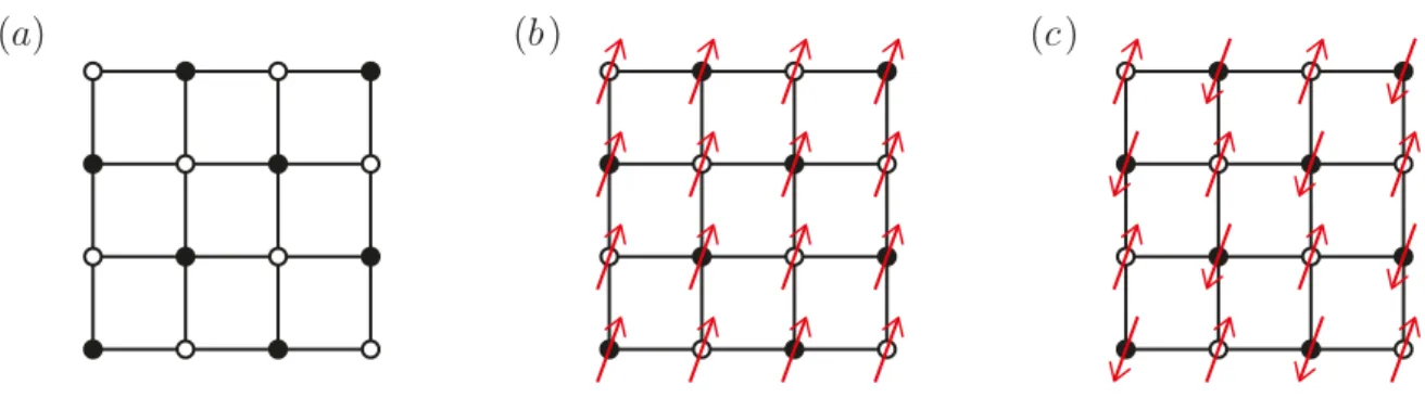
Figure 1.2. Heisenberg model on the square lattice. (a) Bipartite character of the square lattice. The lattice can be divided into two subsets A and B, where each site only has neighbors of the opposite subset. The two different sublattices are indicated by black and white colored lattice sites. (b) Ferromagnetic configuration on the square lattice. At each site, theS^z-component of the spin has the same value. (c) N´eel configuration on the square lattice.

Up and down pointing spins occupy the two sub-lattices Aand B, respectively.

they all have equal strength.

The classical analogue of this model turns out to be fairly simple regardless of the sign of the coupling constant. This is due to the fact that the square lattice is bipartite, which means that the lattice can be sub-divided into two sublattices A and B such that each site in in sublattice Aonly has neighbors in sublatticeB, and vice versa (see Fig. 1.2a).

Ferromagnetic couplings are easily satisfied by a configuration where all spins point in the same direction (Fig. 1.2b). On any bipartite lattice it is also straightforward to satisfy antiferromagnetic couplings by constructing a configuration where the spins on the two sublattices point in opposite directions. Such a configuration is referred to as a N´eel state, see Fig. 1.2c. Both configurations are equivalent (up to the staggered minus sign in the spin orientation) and minimize the energy of their respective Hamiltonian to contribute an exchange energy of −J/4 on every lattice bond. Magnetically ordered phases are therefore particularly favorable on lattices with a large coordination number, i.e. a large number of lattice bonds per spin.

In the quantum model, the ferromagnetic and antiferromagnetic configurations are no longer equivalent. For illustration, let us consider a single pair of quantum spins.

The Heisenberg exchange between the two spins, in terms of spin raising and lowering operators (1.6), is given by

H = J

2 S_i⁺S_j⁻+S_i⁻S_j⁺

+JS_i^zS_j^z . (1.10)

This Hamiltonian has four eigenstates: three triplet states and one singlet state (Fig. 1.3).

The ferromagnetic state in Fig. 1.3a, which we know is also the ground state of the classi- cal model (up to the two-fold degeneracy of all spins pointing up or down, respectively), is an eigenstate of the Hamiltonian (1.10) and minimizes its energy. We note that although the Hamiltonian does not induce transitions between the two degenerate states, thermal fluctuations may still drive a transition. In real systems, however, those transitions are

Figure 1.3. A pair of quantum spins. The Hilbert space of a single spin is two-dimensional.

A system of two such spins is therefore expected to have dimension 4. By convention, the four basis states are grouped into three triplet states, (a) – (c), and one singlet state, (d). The grouping goes back to the fusion rules of angular momenta – two spin-1/2 operators together form either a spin-1 operator (the triplet states withS^z-components -1, 0, and +1) or a spin-0 operator (the singlet state with vanishingS^z-component).

suppressed exponentially in the system size (for two or three-dimensional systems) since the nucleation of a puddle of opposite polarization creates a phase boundary whose de- fect energy scales with the boundary length, such that in the thermodynamic limit only a single configuration is observed.

In contrast, the N´eel configuration is not an eigenstate of the Hamiltonian, which automatically implies additional quantum fluctuations. Furthermore, the energy of a classical antiferromagnetic bond is −J/4 while the energy of an inherently quantum mechanical singlet pair (Fig. 1.3d) is −3J/4, which gives further preference towards quantum fluctuations. Extending the concept of singlet bonds from a single pair of spins to an entire lattice in the thermodynamic limit, one of two things can happen.

Either the outcome is a long-range ordered N´eel configuration, which comes with an energy gain on every bond, but which does not gain energy from singlet fluctuations.

Alternatively, the outcome could be an extension of the singlet state which is constructed by arranging singlet bonds within the lattice such that every spin is part of a singlet pair. The latter minimizes the energy on singlet bonds at the cost of losing potential energy gain on other bonds. It is not easy to make a prediction on which mechanism dominates in the thermodynamic limit. It seems that on bipartite lattice geometries (e.g. the square lattice [19]) the N´eel configuration is the preferred ground state of the Heisenberg antiferromagnet. On non-bipartite lattices the situation can be more complicated, as we shall see in Sec. 1.1.6.

Nevertheless, constructions based on singlet pairs have been discussed extensively in the field of quantum spin liquids. The most straightforward way to construct a macroscopic spin configuration from singlet pairs would be to arrange them in a regular pattern (Fig. 1.4a). Such a state is called a valence bond crystal (VBC). It breaks lattice symmetries and, more importantly, due to its periodic arrangement of singlet bonds it can be broken down into individual, finite clusters. As such, the VBC configuration does not satisfy our expectation for a quantum spin liquid to have massive long-range entanglement. A symmetry preserving construction which cannot be reduced to finite clusters has been proposed by Anderson [20] and is known as the resonating valence bond (RVB) state. It is based on superposing different arrangements of singlet pairs (Fig. 1.4b), leading to highly entangled states of matter which do not break any lattice symmetries. Short-range RVB states have a finite energy gap which corresponds to breaking a single valence bond. However, the construction is not constrained to short-

Figure 1.4. Spin singlet configurations. (a) Valence bond crystal with periodic arrangement of singlet pairs. (b) Resonating valence bond state constructed from the superposition of different arrangements of singlet bonds. (c) Long-range valence bond configuration.

range valence bonds. One can also envision a long-range RVB state where valence bonds go beyond nearest neighbors (see Fig. 1.4c). Such configurations also support gapless low-energy excitations [21].

VBS and RVB states frequently appear in the discussion of frustrated magnetism and spin liquid candidates. Besides emerging as ground state candidates for various conventional spin models, there exist models which are explicitly constructed in a way that favors valence bond configurations. Such quantum dimer models are often described by Hamiltonians that operate on the manifold of all dimer configurations and contain terms which induce transitions between different dimer states [1, 14].

1.1.6 Frustration. We have argued in the previous subsection that singlet configura- tions offer a way to minimize the energy on selected lattice bonds at the cost of losing correlation with spins along other bonds. However, this is often unfavorable on bipartite lattices which are naturally compatible with a N´eel configuration. In order to further suppress magnetic long range order one needs to introduce frustration – a mechanism which, on Hamiltonian level, introduces a set of constraints or exchange couplings which cannot be satisfied simultaneously. Usually, two different kinds of frustration mecha- nisms are distinguished: geometric frustration and exchange frustration.

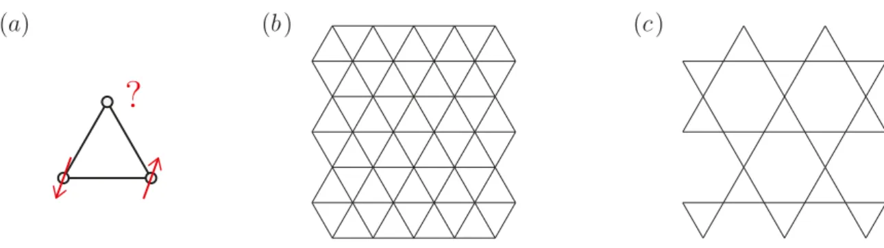
Geometric frustration refers to a situation where a single type of exchange interactions cannot be simultaneously satisfied on all lattice bonds as a consequence of the lattice geometry, even on a classical level. This occurs naturally in non-bipartite lattices with antiferromagnetic interactions, the simplest example being the Heisenberg antiferromag- net on the triangular lattice. On each triangular plaquette the interaction energy can only be minimized on two bonds at a time, while the third bond necessarily violates the antiferromagnetic coupling (at least in the picture of classical spins, see Fig. 1.5a).

The triangular HAFM has been discussed extensively in the past and it seems that the ground state exhibits magnetic long range order despite the presence of quantum fluc- tuations and geometric frustration [22]. Quantum fluctuations are even stronger in a closely related model, the HAFM on the kagome lattice. The kagome lattice is composed of corner sharing triangles, and can be derived from the triangular lattice by depletion of one quarter of the sites (Figs. 1.5b–c). The lower coordination number (four, as op- posed to six in the triangular lattice) and a large classical ground-state degeneracy tilt the scales further away from a magnetically ordered ground state. Indeed, the kagome

Figure 1.5. Geometric frustration. (a) Cartoon picture of geometric frustration. In a triangular plaquette, two spins can be arranged antiferromagnetically. The third spin can only couple antiferromagnetically to one of them, resulting in an energetic penalty on the remaining bond. (b) Triangular lattice. (c) Kagome lattice obtained from the triangular lattice by 1/4 site depletion.

HAFM is widely believed to host a quantum spin liquid ground state [23].

Exchange frustration describes a scenario where multiple competing exchange terms cannot be satisfied simultaneously. Such a situation can be constructed by extending the nearest neighbor Heisenberg model to include interactions between sites that are further apart. A prominent example is the J1J2-Heisenberg model on the square lattice (Fig. 1.6a), which is governed by the Hamiltonian

H =J1

X

hi,ji

S_iS_j +J2

X

hhi,jii

S_iS_j , (1.11)

where hi, ji indicates a sum over nearest neighbors, hhi, jii denotes a sum over next- nearest neighbors, and both coupling constants are chosen to be antiferromagnetic.

When J1 is much larger than J2, the ground state is N´eel ordered, i.e. nearest neighbor spins align antiferromagnetically. On the other hand, when J2 is much larger than J1, the system exhibits collinear order where next-nearest neighbors align antiferromagnet- ically. As a result of the competing interactions there exists a regime without magnetic long range order between J2/J1 ≈0.4 and J2/J1 ≈ 0.6, whose true nature is still under debate [1].

An alternative way to generate exchange frustration which has grown very popular since the conception of the Kitaev honeycomb model [4] is to define bond-dependent exchange terms where different spin components are coupled along different bond types.

For illustration, consider the Kitaev honeycomb Hamiltonian H=K X

hi,ji_γ

S_i^γS_j^γ , (1.12)

where hi, jiγ runs over nearest neighbors on the tricoordinate honeycomb lattice and γ labels the three types of bonds emanating from each lattice site byx,y, andzas depicted in Fig. 1.6b. Already on a classical level frustration arises from the length constraint

Figure 1.6. Exchange frustration. (a) Exchange frustration in theJ1J2-Heisenberg model on the square lattice. Solid lines denote interactions of strength J₁, dashed lines representJ₂. Antiferromagnetic coupling cannot be simultaneously satisfied for both types of interactions.

(b) Exchange frustration in the Kitaev honeycomb model. Thex-component of spin operators is coupled along red lattice bonds, the y and z components along green and blue bonds, respectively.

of a spin since it cannot maximize all three components simultaneously; quantum spins naturally introduce further quantum fluctuations. The Kitaev honeycomb model is one of the few models with a quantum spin liquid ground state, where the existence of a quantum spin liquid ground state can be proven analytically [4].

1.2. Simulation techniques for spin liquids

There is only a limit set of techniques available which are suited for the analysis of frus- trated quantum magnetism and which remain largely unbiased towards either magnetic ordering tendencies or spin liquid behavior. Three prominent examples among them are (i) exact diagonalization, (ii) different flavors of quantum Monte Carlo techniques, and (iii) the density matrix renormalization group. These methods significantly contribute to the foundation on which modern (numerical) studies of strongly correlated systems are built. In this section we briefly review main aspects of the different techniques, their strengths and their shortcomings. The goal of this section is to provide some context in the landscape of methods in condensed matter theory – and to convey a feeling of when it is appropriate to utilize these established methods, and when the situation might call for a different approach.

1.2.1 Exact diagonalization. Exact diagonalization (ED) can be considered the most direct way to approach a quantum many-body system. It is the brute force way of exactly computing all eigenstates and eigenenergies of an arbitrary Hamiltonian by the numerical diagonalization of the Hamilton matrix acting on a finite dimensional Hilbert space. This has two implications: firstly, the Hilbert space has to be finite. For lattice spin models one needs to operate on lattice graphs with a finite number of sites, which necessarily introduces a boundary to the system. Yet, one may vary the nature of the boundary conditions (make them open boundary conditions or periodic boundary

conditions) and perform a systematic finite-size analysis to obtain an estimate of the impact of boundaries on the bulk system.

The second implication is that one needs to express the model in an explicit basis of the Hilbert space. A straightforward way of doing this is to rewrite spin operators in terms of spin raising and lowering operators, thus formulating everything in the S^z basis (see Sec. 1.1.4). Every spin on the lattice has a local basis of two dimensions, and the total Hilbert space for a lattice of N spins grows exponentially as 2^N. Consequently, the associated Hamilton matrix acting on the Hilbert space has dimension 2^N ×2^N. The diagonalization of the Hamilton matrix amounts to the solution of the Schr¨odinger equation H|ψi = Eψ|ψi in the Hilbert space of enumerated spin configurations |ψi =

σ^z₁. . . σ₂^zN

. With the knowledge of all eigenstates it is possible to compute any physical properties of the system, at least in principle. However, due to the exponentially large size of the Hamilton matrix one is restricted to very small system sizes and even after a careful finite-size extrapolation the results may still be severely affected by boundary effects.

Although the overall system sizes which are amenable to treatment by ED remain relatively small, some improvements over the brute force approach are possible. Making use of symmetries and the associated conserved quantities of the Hamiltonian allows a significant reduction of the computational costs of the solution. In the ED formulation, symmetries have a direct impact on the structure of the Hamiltonian matrix; it assumes a block-diagonal form where each block is associated with a fixed set of conserved quan- tities and any transitions between different configurations can only occur within that block. Such a block-diagonal structure can be diagonalized more efficiently. Further- more, one often is only interested in low-lying eigenstates of the system, i.e. states with the lowest associated eigenvalues. In order to obtain them it is not necessary to diagonalize the Hamiltonian matrix exactly, but one can make use of algorithms that approximately compute only the low-energy states, e.g. the Lanczos algorithm [24].

Yet, if one is interested in thermodynamic behavior or excited states in general, precise knowledge of all eigenstates is inevitable.

In summary, the advantage of ED is its applicability to arbitrary systems with the only limitation being severe restrictions on the system size. ED studies are often sufficient to obtain insight into two-dimensional quantum magnets, but complex three-dimensional lattice models where already a single unit cell of the lattice can become quite large remain out of reach.

1.2.2 Quantum Monte Carlo. The simulation of quantum magnetism by means of Monte Carlo (MC) techniques is very desirable. MC techniques are stochastic approaches and as such they generate statistical errors. Yet, the error is well controlled and con- verges towards zero in the limit of long run-times of the simulation; hence, the notion of run-time (or simulation time) is a central measure in MC calculations. The main idea of MC is to generate a finite set of configurations whose statistical distribution adheres to the Boltzmann distribution of the system in thermal equilibrium. The amount of simulation time which has been invested in the calculation directly enters in the number

of configurations which can be generated. In general, the total configuration space is exponentially large, and computing the Boltzmann distribution of all configurations thus is exponentially difficult (c.f. the discussion of exact diagonalization) – within Monte Carlo, however, meaningful results can be achieved in much shorter time by efficiently sampling only a subset of the configuration space, weighted by the Boltzmann distribu- tion. Configurations which are more likely to appear in a real system and therefore have a relatively large impact on observable quantities are also likely to appear in the finite sample of configurations generated in a MC simulation.

Classical magnetism can often be efficiently simulated via Monte Carlo. The trick which allows MC to sample arbitrary probability distributions efficiently is to generate a chain of configurations by iteratively applying local changes until the configurations effectively become independent of each other. The procedure of iteratively applying local changes becomes difficult near phase transitions – in proximity to a phase transition the intrinsic length scale of the system (the correlation length) may diverge and cause fluctuations on all length scales to become equally relevant. Further problems may arise for example in spin glass phases where an extensive number of local energy minima slows down the simulation dramatically and causes it to remain in local energy minima for a significant amount of simulation time. Just like exact diagonalization, MC explicitly operates on the phase space of spin configurations, and thus only finite lattice graphs can be simulated. The system size which can be simulated in MC is much larger than in ED, but in certain models boundary conditions may still become relevant. In chapter 3.1 we discuss such an example where the ground state is characterized by the formation of incommensurate spiral patterns, i.e. spin configurations which are neither compatible with open boundary conditions nor with periodic boundary conditions.

For quantum systems, the set of models that withstand an efficient solution via Monte Carlo techniques is much larger. The non-trivial commutation relations in fermionic quantum many-body systems can lead to negative statistical weights, but the MC al- gorithm can only work efficiently for positive definite weights – otherwise terms with opposite weight cancel, resulting in a fatal slowdown of statistical error convergence.

This is referred to as the ‘sign problem’ in quantum Monte Carlo. It is often the highly frustrated quantum spin models of interest, which are plagued by the sign problem. Yet, specialized quantum Monte Carlo algorithms have been demonstrated to overcome the sign problem in certain cases, e.g. for the Hubbard model on bipartite lattices [25], or for the Kitaev honeycomb model [26].

Not relying on any severe approximations, quantum Monte Carlo often is the tool of choice for models which are sign-problem free.

1.2.3 Density matrix renormalization group. A third, popular technique in the description of quantum many-body systems is the density matrix renormalization group (DMRG) [27, 28], which is conceptionally very different from the previous two methods.

DMRG outlines an algorithm to iteratively adjust and trim the number of internal degrees of freedom in a quantum many-body system as a way to retain only the most relevant bits of information, hence the reference to ‘renormalization group’ in the naming.

In its modern interpretation, different flavors of DMRG exist that may either aim to describe infinite systems (infinite-system DMRG) or operate on finite systems (finite- system DMRG). The latter can be understood also as an optimization problem with the goal to describe a physical spin configuration in terms of a (position dependent) matrix product state.

An arbitrary quantum mechanical wave function which describes a cluster of N quan- tum mechanical spins, where each spin at position i has its local configuration space {σi}={↑,↓}, is approximated by the matrix product state

|ψi= X

σ1...σN

Tr

N

Y

i=1

Ai[σi]

!

|σ1. . . σNi , (1.13) where DMRG provides a way to determine the entries of the M ×M matrices Ai[σi].

The quality of the approximation depends on the dimensionM of these matrices (which also determines the computational complexity of the algorithm) as well as on the speed at which the eigenvalues of the matrix decay. The eigenvalue scaling can be one of the four qualitatively different scenarios [28]: (i) In the best case scenario the true eigenstate of the system is represented by a matrix product state. In this case there is only a finite number of non-zero eigenvalues and DMRG is able to represent the exact solution. (ii) Similarly well behaved is the scenario of exponentially fast decaying eigenvalues, which is the case for one-dimensional gapped quantum systems. Under these circumstances DMRG is still able to efficiently capture the relevant physics and to predict observables with an accuracy close to machine precision. (iii) It gets more difficult when the decay of eigenvalues slows down with increasing system size, which is the case for critical one-dimensional quantum systems. The slow decay of eigenvalues for larger systems implies that DMRG is unable to faithfully capture the thermodynamic limit in these systems. (iv) In two dimensions and higher, the number of relevant eigenvalues grows with increasing system size. These systems are most difficult to treat in DMRG.

In practice, one may estimate the truncation error which results from finite matrix dimensionsM by comparing calculations at different values for the dimensionalityM of the matrix product states at any given system size. Being able to estimate numerical errors it is still possible to make predictions about two-dimensional systems, despite the scaling behavior of relevant eigenvalues being unfavorable. One is, however, restricted to relatively small systems – this is also the reason that DMRG studies of two-dimensional systems are usually only performed on stripe (or cylinder) geometries, keeping the total system size small and at the same time making the system quasi one-dimensional.

In summary, DMRG is very powerful for most one-dimensional systems, yielding re- sults of remarkable precision. For systems of this kind, DMRG is the method of choice.

Unlike Monte Carlo, DMRG does not know a sign problem and hence may also be applied to frustrated quantum magnets. Despite its reduced performance in two di- mensions, DMRG is an immensely valuable tool also in the field of two-dimensional frustrated quantum magnetism, in particular for models which are not amenable to a treatment by Monte Carlo. In recent years, the use of DMRG has helped to reach im-

portant milestones in the research of quantum spin liquids. For example, with the help of DMRG, unambiguous evidence for the existence of a chiral spin liquid on the kagome lattice with Heisenberg interactions up to third neighbors has been provided [29, 30].

Furthermore, the use of DMRG has made valuable contributions to the discussion of the kagome Heisenberg antiferromagnet, with current simulations making a strong point that the ground state is a gapless U(1)-Dirac spin liquid [23]; these contributions, how- ever, also spotlight the subtleties of DMRG in two dimensions. Discriminating the two competing proposals of a gapless U(1) and a gapped Z² spin liquid might sound sim- ple, but it has proven to be a great challenge in finite cylinder geometries, and a lot of thought has to be put into understanding the impact of boundary conditions. Finally, employing DMRG may also give direct access to subtle properties like the entanglement structure in two-dimensional quantum many-body systems. Three dimensional systems, however, are much less well behaved and are currently out of reach for DMRG.

1.2.4 Functional renormalization group. Throughout the remainder of this thesis, the method of choice is going to be the pseudo-fermion functional renormalization group (pf-FRG), which is a relatively new addition to the toolset of numerical approaches in frustrated quantum magnetism. We have seen in the previous discussions that the main workhorses in the numerical study of frustrated quantum magnetism are often not suited to faithfully describe three-dimensional frustrated quantum magnets, leaving a methodological void in the field. In the next part of the thesis, Chapter 2, we introduce the pseudo-fermion functional renormalization group formalism, which we shall see can also be applied to simulate frustrated quantum magnetism in three spatial dimensions;

the chapter is dedicated to a pedagogical introduction to the method itself, the theory behind it, and its practical implementation. Thereafter, in Chapter 3, we provide sev- eral examples from the field of frustrated quantum magnetism where we study model Hamiltonians that support the emergence of quantum spin liquid phases – guided by applications to real materials.

renormalization group

In the previous chapter we have discussed some of the most pervasive techniques in the field of frustrated quantum magnetism: exact diagonalization, quantum Monte Carlo, and the density matrix renormalization group. All of these methods are quite powerful in the study of two-dimensional frustrated magnetism. Yet, exact diagonalization and density matrix renormalization group are not suitable for applications in three dimen- sions, and quantum Monte Carlo is often impaired by the infamous sign problem when applied to models of frustrated magnetism.

A complementary numerical approach has been pursued by Reuther and W¨olfle (2010) [6]: the pseudo-fermion functional renormalization group (pf-FRG). In its early days the method has been successfully applied to various paradigmatic models of frustrated quantum magnetism in two dimensions, ranging from the triangular antiferromagnet [31] via the kagome antiferromagnet [32] to the Kitaev honeycomb model [33], and more [34, 35]. In the continuous development of the approach it was quickly realized that the method is straightforwardly applicable also to three-dimensional frustrated quantum magnetism [36], allowing access to prototypical models of frustration on the hyperkagome lattice [P1] and on the pyrochlore lattice [37]. The great success in the study of a long list of archetypal examples of frustrated magnetism has demonstrated that the pf-FRG offers a promising perspective and can help to diminish the methodological void around the field of frustrated quantum magnetism in three dimensions.

While in the early days of pf-FRG the use of the method has been justified mostly by its successful applications, in more recent days additional insight has been gained into the validity of the approximation schemes which the approach is built on. For example, it has been shown that the pf-FRG becomes exact in the classical limit of large spins [38] as well as in the large-N limit of enhanced SU(N) spin symmetry [P2, P3].

Moreover, the pf-FRG has been further refined to be applicable to models with less symmetric off-diagonal spin interactions including, but not limited to, Dzyaloshinskii- Moriya interactions [39, P6, P7]. Unrelated to the original formulation of pf-FRG, efforts are being made in the development of a functional renormalization group scheme which operates directly on the internal spin degrees of freedom instead of re-casting them in terms of pseudo-fermions [40]. The latter approach is a very recent development and it remains to be seen how feasible it is in practical calculations.

The aim of this chapter is to review the theory behind the pseudo-fermion functional renormalization group (pf-FRG), putting strong emphasis on its practical application.

Understanding pf-FRG is a three step process which can be broken down into (i) the

derivation of the general functional renormalization group (FRG) flow equations, (ii) the construction and symmetry analysis of the pseudo-fermion Hamiltonian which acts as a fermionic representation of the spin Hamiltonian, and (iii) refining the general functional renormalization group scheme by implementing specific symmetries and approximation schemes for the pseudo-fermionic model. We address the first step only briefly. There al- ready exists an extensive body of literature on the general formulation of the functional renormalization group with applications of FRG covering not just condensed matter systems but also being influential in high-energy physics and quantum gravity [41]; a pedagogical review of the general formalism would fill a book on its own. For more details on the general concept of the functional renormalization group we instead refer the reader to text books [42], review articles [43–45], or influential papers [46] on the subject. A lot of work has been done on FRG implementations for fermionic models in condensed matter theory and there is a long record of discussions of different approx- imation schemes and their validity. However, making the transition from conventional fermionic systems to pseudo-fermionic models, which we shall see have very different symmetry implications compared to regular fermions, requires us to re-evaluate the ap- plicability of approximation schemes. Therefore our focus is put on the discussion of original aspects about the pf-FRG which go beyond the implementation of conventional fermionic FRG schemes.

After a brief general introduction to the functional renormalization group in Sec. 2.1 we discuss the characteristic properties of the pseudo-fermion Hamiltonian in Sec. 2.2. In Sec. 2.3 we derive the pf-FRG flow equations, followed by a discussion of their numerical solution (Sec. 2.4) and selected aspects about the interpretation of pf-FRG calculations (Sec. 2.5).

2.1. Functional renormalization group

Conceptually, the functional renormalization group (FRG) can be thought of as the rewriting of a functional integral, which serves as a central object in many-body quantum field theories from which physical observables may be computed,

Z = Z

D( ¯ψ, ψ)e^−S0−Sint , (2.1) into an infinite hierarchy of integro-differential equations

d

dΛγm(k1⁰, . . . , km⁰;k1, . . . , km) =Fm^Λ(γ0, γ2, γ4, . . . , γm+2) , (2.2) where the expressions Fm on the right hand side of the equation can be complicated non-linear integral expressions (their precise form and notation is introduced later in this chapter). We shall see below that the rewriting is exact and that both formulations – the functional integral expression and the differential equation – thus contain the same information. Both formulations are intrinsically difficult to solve for strongly interact- ing many-body systems: the functional integral contains a sizable quartic contribution Sint which spoils the solubility of the Gaussian integral, while the differential equations cannot be solved because their structure is an infinite hierarchy of coupled expressions.

In non-interacting systems, on the other hand, both formulations are inherently simple.

The functional integral becomes Gaussian, while the initial conditions of the differential equations are such that only a single component can become non-zero, while all other orders in the infinite hierarchy vanish.

Operating in a regime which lies in between non-interacting systems and strongly interacting systems one needs to lean on approximation schemes which are often well behaved in the weak coupling limit and become less controlled as the interaction strength is increased. In this regime the liberty to switch between the integral formalism and the differential formalism becomes immensely valuable because both approaches are amenable to different approximation schemes. While the functional integral formulation is often used in combination with traditional renormalization group (RG) schemes in order to determine a small set of renormalized interaction constants, the FRG approach provides an overarching concept for the renormalization of much larger sets of interaction parameters (c.f. Fig. 2.1) which defines a natural language to compute diagrammatic resummations of interaction vertices.

In the remainder of this section we derive the general form of fermionic FRG flow equations. For the derivation we closely follow the steps as outlined in Ref. [43]. The same conceptional steps are also described in textbook style with more elaborate com- mentary in Ref. [42] – however, their notation is overly complicated for our purpose since they operate in a superspace of combined fermionic and bosonic theories where the particle number is no longer preserved.

As a starting point for our derivation we consider a general fermionic model with quartic interactions whose HamiltonianH =H0+Hintcan be split into two contributions