Stream Compaction

(1)

G. Zachmann Massively Parallel Algorithms SS 20 June 2013 Preﬁx-Sum 45

Stream Compaction

§ 

Given: input stream A, and a ﬂag/predicate for each a_i

§ 

Goal: output stream A' that contains only a_i's, for which ﬂag = true

§ 

Example:

§  Given: array of upper and lower case letters

§  Goal: delete lower case letters and compact the upper case to the low-order end of the array

§  

Solution:

§  Just like with the split operation, except we don't compute indices for the

"false" elements

§  

Frequent task: e.g., collision detection,

§  

Sometimes also called list packing, or stream packing

A x C P h b B z

a:

1 0 1 1 0 0 0 1

a':

A C P B

b:

(2)

Summed-Area Tables / Integral Images

§ 

Given: 2D array T of size w×h

§ 

Wanted: a data structure that allows to compute

for any i₁, i₂, j₁, j₂ in O(1) time

i₂

k=i₁ j₂

l=j₁

T(k,l)

i1 i₂

j₂ j₁

(3)

§ 

The trick:

§ 

Deﬁne

§ 

With that, we can rewrite the sum:

i₂

k=i₁ j₂

l=j₁

T(k,l) =

i₂

k=1 j₂

l=1

T(k,l)

i₁

k=1 j₂

l=1

T(k,l)

i₂

k=1 j₁

l=1

T(k,l)

+

i₁

k=1 j₁

l=1

T(k,l)

S(i, j) =

i

k=1 j

l=1

T(k,l)

i₂

k=i1

j₂

l=j1

T(k,l) = S(i2,j2) S(i1,j2) S(i2,j1) + S(i1,j1)

(0,0)

+

+ -

-

Lookups in

Summed Area Table S

(4)

§  

Deﬁnition:

Given a 2D (k-D) array of numbers, T, the summed area table S stores for each index (i,j) the sum of all elements in the rectangle (0,0) and (i,j) (inclusively):

§ 

Like preﬁx-sum, but for higher dimensions

§ 

In computer vision, it is often called integral image

§ 

Example:

Input

1 1 0 2 1 2 1 0 0 1 2 0 2 1 0 0

1 2 2 4 2 5 6 8 2 6 9 11 4 9 12 14

Summed Area Table

S(i, j) =

i

k=1 j

l=1

T(k,l)

(5)

§  

The algorithm: 2 phases (for 2D)

1.  Do H preﬁx-sums horizontally 2.  Do W preﬁx-sums vertically

-  Real implementation (to maintain coalesced memory access):

preﬁx-sum vertically, transpose, preﬁx-sum vertically -  Or use texture memory

§ 

Depth complexity for k-D (assume w = h, and "native"

horizontal preﬁx-sum, i.e., no transposition):

§  

Caveat: precision of integer/ﬂoating-point arithmetic

§  Assumption: each T_ij needs b bits

§  Consequence: number of bits needed for S_wh =

§  Example: 1024x1024 grey scale input image, each pixel = 8 bits

→ 28 bits needed in S-pixels

k·W log W

log w + log h + b

(6)

Increasing the Precision

§ 

The following techniques actually apply to preﬁx-sums, too!

1. "Signed offset" representation:

§  Set

where

§  Effectively removes DC component from signal

§  Consequence:

i.e., the values of S' are now in the same order as the values of T (less bits have to be thrown away during the summation)

§  Note 1: we need to set aside 1 bit (sign bit)

§  Note 2: S'(w,h) = 0 (modulo rounding errors)

T⁰(i,j) = T(i, j)–¯t

¯t = average of T = _{w h}¹ P_w

1

P_h

1 T(i, j)

S⁰(i,j) =

Xi

k=1

Xj

l=1

T⁰(k,l) = S(i, j) i·j·¯t

(7)

§ 

Example:

input texture original summed-area table this work input texture original summed-area table this work

input texture original summed-area table this work

Input image Original summed area table

Improved precision using "offset" representation

(8)

2.  Move the "origin" of the i,j "coordinate frame":

§  Compute 4 different S-tables, one for each quadrant

§  Result: each S-table comprises only ¼ of the pixels/values of T

§ 

For computation of do a simple case switch

i j

i₁ i₂

j₂

j₁ i

j

Pi₂ k=i₁

Pj₂

l=j₁ T(k,l)

(9)

Results

§ 

Compute integral image

§ 

From that, compute

§  I.e., 1-pixel box ﬁlter

§  

Should yield the original image (theoretically)

J. Hensley, T. Scheuermann, G. Coombe, M. Singh & A. Lastra / Fast Summed-Area Table Generation and its Applications

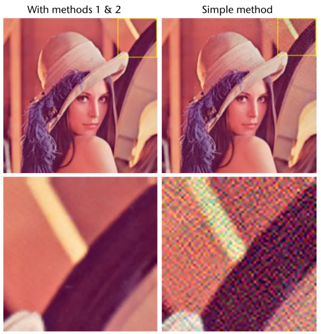
Figure 4: The left column shows the original input images, the middle column are reconstructions from summed-area tables (SATs) generated using our method, and the right column are reconstructions from SATs generated with the old method. For the first row, the SATs are constructed using 16 bit floats, for the second row the SATs are constructed using 24 bit floats, and the final row shows a zoomed version of second row (region-of-interest highlighted)

first row shows three versions of a checkerboard. The image on the right, generated using the traditional method, ex- hibits unacceptable noise throughout much of the image. In contrast, the middle image, generated by our method, barely shows error.

Centering around image pixel average. While centering pixel values around the 50% gray level proved to be quite useful, an even better approach is to store offsets from the image’s average pixel value. This is especially true of images

such as Lena for which the image average can be quite different from 50% gray. For such images, centering around 50%

gray could still result in sizable magnitudes at each pixel po- sition, thereby increasing the probability that the summed- area values could appreciably grow in magnitude. Centering the pixel values around the actual image average guarantees that the summed-area value is equal to 0 both at the origin and at the upper right corner (modulo floating-point rounding errors).

c The Eurographics Association and Blackwell Publishing 2005.

S(i,j) S(i 1,j) S(i,j 1) +S(i 1,j 1)

Simple method With methods 1 & 2

(10)

§ 

Naïve approach: do a 1D preﬁx-sum per row →

depth complexity (assuming we omit the matrix transposition step) and work complexity,

where input image has size n×n = N pixels

§ 

Better solution:

§  Pack all rows into one linear array of size N

§  Do a 1D preﬁx-sum, but only the ﬁrst n levels

→ depth complexity

§  Work complexity =

§ 

Is a special case of

segmented preﬁx sum

O N

Row 1 Row 2 Row n

n levels up- and down- sweep

Efﬁcient Computation of the Integral Image

O p

N log N O p

N ·p

N = O N

O logN

(11)

Applications of the Summed Area Table

§ 

For ﬁltering in general

§ 

Simple example: box ﬁlter

§  Compute average inside a box (= rectangle)

§  Slide box across image (convolution)

§ 

Application: translucent objects, i.e., transparent & matte

§  E.g., milky glass

1.  Render virtual scene (e.g., game) without translucent objects 2.  Compute summed area table from frame buffer

3.  Render translucent object (using fragment shader): replace pixel behind translucent object by average over original image within a (small) box

(12)

§ 

Result:

(13)

Rendering with Depth-of-Field (Tiefenunschärfe)

1.  Render scene, save color buffer and z-buffer (e.g., in texture) 2.  Compute summed area table over color buffer

3.  For each pixel do in parallel:

1. Read depth of pixel from saved z-buffer 2. Compute circle of confusion (CoC)

(for details see "Advanced CG") 3. Determine size of box ﬁlter

4. Compute average over

saved color buffer within box 5. Write in color buffer

§  

Note: "For each pixel in parallel"

could be implemented in OpenGL

by rendering a screen-ﬁlling quad using special fragment shader

(14)

§ 

Result:

3/8/13 11:34 AM GPU Gems 3 - Chapter 39. Parallel Prefix Sum (Scan) with CUDA

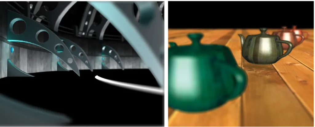
the lower-left corner sample, and so on (Crow 1977). We can use this technique for variable-width filtering, by varying the locations of the four samples we use to compute each filtered output pixel.

Figure 39-12 shows a simple scene rendered with approximate depth of field, so that objects far from the focal length are blurry, while objects at the focal length are in focus. In the first pass, we render the teapots and generate a summed-area table in CUDA from the rendered image using the technique just described. In the second pass, we render a full-screen quad with a shader that samples the depth buffer from the first pass and uses the depth to compute a blur factor that modulates the width of the filter kernel. This determines the locations of the four samples taken from the summed-area table at each pixel.

Figure 39-12 Approximate Depth of Field Rendered by Using a Summed-Area Table to Apply a Variable-Size Blur to the Image Based on the Depth of Each Pixel

Rather than write a custom scan algorithm to process RGB images, we decided to use our existing code along with a few additional simple kernels. Computing the SAT of an RGB8 input image requires four steps. First we de-interleave the RGB8 image into three separate floating-point arrays (one for each color channel). Next we scan all rows of each array in parallel. Then the arrays must be transposed and all rows scanned again (to scan the columns). This is a total of six scans of width x height ele- ments each. Finally, the three individual summed-area tables are interleaved into the

(15)

Artifacts of this Technique

§ 

False sharp silhouettes: blurry objects (out of focus) have sharp silhouette, i.e., won't blur over sharp object (in focus)

§ 

Color bleeding (a.k.a. pixel bleeding): areas in focus can incorrectly bleed into nearby areas out of focus

§ 

Reason: the (indiscriminate) gather operation

(16)

§ 

Goal: turn gather operation into scatter operation

§ 

Example: scatter one pixel using the 2D preﬁx-sum (integral image)

Depth-of-Field with Scattering

0.2 0.5 0.7 0.5 0.2

0.14 0.14 0.14 0.14 0.14 0.2 0.5 0.7 0.5 0.2

0.42

orig.

image

blurred image

average gathered over CoC one pixel scattered over CoC

Input image with one pixel set and its "circle"-of-confusion

0.9

+0.1 -0.1

-0.1 +0.1

Pixel value spread to the corners of the rectangle

0.1

0.1 0.1 0.1 0.1 0.1 0.1 0.1 0.1

Resulting 2D preﬁx-sum

= pixel scattered over CoC

(17)

Algorithm

1.  Phase: for each pixel in original image do in parallel

§  Spread to CoC corners

-  Use atomic accumulation operation ! -  Do this for each R, G, and B channel

2.  Phase: compute 2D preﬁx-sum, result = blurred image

§  

Question: can you turn phase 1 into a gather phase?

pixel value area(CoC)

(18)

Result

Summed area table and gathering Scattering and 2D preﬁx-sum

[Kosloff, Tao, Barsky, 2009]

(19)

Recap: Texture Filtering in Case of Miniﬁcation

§ 

What happens, when we "zoom away" from the polygon?

Miniﬁcation (texels are small compared to pixels)

Magniﬁcation (texels are large compared to pixels)

Texture

u v

(20)

§  Linear interpolation does not help very much:

§  Needed would be an averaging of all texels covered by the pixel (in uv-space); too costly in real-time

§  Solution: pre-processing → MIP-Maps

(lat. "multum in parvo" = Vieles im Kleinen")

Take texel closest to pixel center (in u,v) Linear interpolation of 4 texels closest to pixel ctr

(21)

§  

A MIP-Map is just an image pyramid:

§  Each level is obtained by averaging 2x2 pixels of the level below

-  Consequence: the original image must have size 2ⁿx2ⁿ (at least, in practice)

§  You can use more sophisticated ways of ﬁltering, e.g., Gaussian

§ 

Memory usage for MIP-Map: 1.3x original size

(22)

Anisotropic Texture Filtering

§ 

Problem with MIPmapping: doesn't take the

"shape" of the pixel in texture space into account!

§  MIPmapping just puts a square box around the pixel in texture space and averages

all texels within

§  

Solution: average over bounding rectangle

§  Use Summed Area Table for quick summation

§  Question: how to average over highly "oblique" pixels?

Mip Maps

• Keep textures prefiltered at multiple resolutions

o For each pixel, use the mip-map closest level o Fast, easy for hardware

• This type of filtering is isotropic:

o It doesnʼt take into account that there is more compression in the vertical direction than in the horizontal one

Again: we’re trading aliasing for blurring!

s t

Mip Maps

• Keep textures prefiltered at multiple resolutions

o For each pixel, use the mip-map closest level o Fast, easy for hardware

• This type of filtering is isotropic:

o It doesnʼt take into account that there is more compression in the vertical direction than in the horizontal one

Again: we’re trading aliasing for blurring!

s t

Mip Maps

• Keep textures prefiltered at multiple resolutions

o For each pixel, use the mip-map closest level o Fast, easy for hardware

• This type of filtering is isotropic:

o It doesnʼt take into account that there is more compression in the vertical direction than in the horizontal one

Again: we’re trading aliasing for blurring!

s

t

(23)

§ 

This is one kind of anisotropic texture ﬁltering

§ 

Result:

No ﬁltering

Mipmapping

Summed area table

(24)

§ 

Another example:

§ 

Today: all graphics cards support anisotropic ﬁltering (not necessarily using SATs)

Mipmapping Anisotropic

(25)

Application: Face Detection

§ 

Goal: detect faces in images

§  

Requirements (wishes):

§  Real-time or close (> 2 frames/sec)

§  Robust (high true-positive rate, low false-positive rate)

§  

Non-goal: face recognition

§  

In the following: no details, just overview!

digital camera iPhoto "False positive" from

human point of view

(26)

§ 

The term feature in computer vision:

§  Can be literally any piece of information/structure present in an image (somehow)

§  Binary features → present / not present;

examples:

-  Edges (e.g., gradient > threshold)

-  Color of pixels is within speciﬁc range (e.g., skin) -  Ellipse ﬁlled with certain amount of skin color pixels

§  Non-binary features → probability of occurrence;

examples:

-  Gradient image

-  Sum of pixel values within a shape, e.g., rectangle

(27)

The Viola-Jones Face Detector

[2002]

§ 

The (simple) idea:

§  Move sliding window across image (all possible locations, all possible sizes)

§  Check, whether a face is in the window

§  We are interested only in windows that are ﬁlled by a face

§  

Observation:

§  Image contains 10's of faces

§  But ~10⁶ candidate windows

§  

Consequence:

§  To avoid having a false positive in every image, our false positive rate has to be < 10^-6

(28)

§ 

Feature types used in the Viola-Jones face detector:

§  2, 3, or 4 rectangles placed next to each other

§  Called Haar features

§ 

Feature value := g_i =

pixel-sum( white rectangle(s) ) – pixel-sum( black rectangle(s) )

§  Constant time

per feature extraction

§ 

In a 24x24 window, there are

~160,000 possible features

-  All variations of type, size, location within window

6 reads from the integral image

8 reads from the integral image

(29)

§ 

Deﬁne a weak classiﬁer for each feature:

§  "Weak" because such a classiﬁer is only slightly better than a random "classiﬁer"

§  

Goal: combine lots of weak classiﬁers to form one strong classiﬁer

f₁ f₂

fi =

(+1 ,g_i > ✓_i 1 , else

F (window) = ↵

₁

f

₁

+ ↵

₂

f

₂

+ . . .

(30)

§ 

Use learning algorithms to automatically find a set of weak classifiers and their optimal weights and thresholds, which together form a strong classifier (e.g., AdaBoost)

§  More on that in AI & machine learning courses

§  

Training data:

§  Ca. 5000 hand labeled faces

-  Many variations (illumination, pose, skin color, …)

§  10000 non-faces

§  Faces are normalized (scale, translation)

§ 

First weak classiﬁers with largest weights are meaningful and have high

discriminative power:

§  Eyes region is darker than the upper-cheeks

§  Nose bridge region is brighter than the eyes

(31)

§ 

Arrange in a ﬁlter cascade:

§  Classiﬁer with highest weight comes ﬁrst

-  Or small sets of weak classiﬁers in one stage

§  If window fails one stage in cascade

→ discard window

-  Advantage: "early exit" if "clearly" non-face

§  Typical detector has 38 stages in the cascade,

~6000 features

§  

Effect: more features → less false positives

§  Typical visualization:

Receiver operating

characteristic (ROC curve)

Stage 1

Stage 2

Stage K

No Maybe

Maybe

Almost certainly

vs false neg determined by

% False Positives

% True Positives

0 50

0 100

No

(32)

§ 

Final stage: only report face, if cascade ﬁnds several nearby face windows

§  Discard "lonesome" windows

(33)

Visualization of the Algorithm

Adam Harv

(http://vimeo.com/12774628)

(34)

Final remarks on Viola-Jones

§ 

Pros:

§  Extremely fast feature computation

§  Scale and location invariant detector

-  Instead of scaling the image itself (e.g. pyramid-ﬁlters), we scale the features

§  Works also for some other types of objects

§  

Cons:

§  Doesn't work very well for 45˚ views on faces

§  Not rotation invariant

(35)